MINOS Observations of Shadowing in the Muon Flux Underground

Abstract

A high significance observation of two muon signals, the shadow of the sun and moon, have been seen by the 5.4 kt MINOS Far Detector, at a depth of 2070 mwe. The distribution of angular separation of muons near the moon was well described by a Gaussian, which was used to determine the angular resolution ($0.34^{\circ}\pm 0.07^{\circ}$) and pointing ($0.3^{\circ}\pm 0.05^{\circ}$) of the detector.

1 Introduction & Motivation

The MINOS Far Detector is a magnetized scintillator and steel calorimeter, located in the Soudan Mine in northern Minnesota, USA, at a depth of 720 m. While primary function of the Far Detector is to detect neutrinos from Fermilab’s $\nu_{\mu}$ beam, the great depth and wide acceptance of the detector combined with the flat overburden of the Soudan site allow it to serve as a cosmic-ray muon detector as well. The detector is composed of 486 8 m octagonal planes 2.54 cm thick, spaced 5.96 cm. This 5.4 kt detector is 30 m long and has a total aperture of $6.94\times 10^{6}\,\mathrm{cm^{2}~{}sr}$. MINOS is the first underground experiment able to discriminate positively charged particles from those that are negatively charged for the purpose of CPT violation investigations, but this feature also allows independent study of positively and negatively charged cosmic rays.

Optical telescopes use a standard catalogue of stars to establish the resolution and pointing reliability of a new instrument. This is not possible for a cosmic ray detector, as there are no cosmic ray sources available for calibration. There are two well observed phenomena in the otherwise isotropic cosmic ray sky, though they are deficits, not sources. The sun and the moon provide a means to study the resolution and pointing of a cosmic ray detector because they absorb incident cosmic rays, causing deficits from their respective location. These signals allow a measure of phenomena associated with cosmic ray propagation and interaction resulting from geomagnetic fields, interplanetary magnetic fields, multiple Coulomb scattering, etc. These extra-terrestrial objects have the same $0.5^{\circ}$ diameter as viewed from Earth, though the sun shadow is more difficult to observe because is much farther away and has its own magnetic field that deflects the charged cosmic rays. The cosmic ray shadow of the moon has been measured by air shower arrays (CYGNUS  [1], CASA [2] , Tibet [3] ), as well as underground detectors (Soudan 2 [4], MACRO [5, 6], L3+C [7]).

2 Data

This analysis encompassed events recorded over 1339 days, from 1 August 2003 - 31 March 2007, for a total of 1194 live-days, and includes 51.41 million cosmic ray induced muon tracks. Cosmic ray muons were triggered by recording hits on 4/5 planes or exceeding a pulse-height threshold and were written to a temporary disk at Soudan and later sent to Fermilab for reconstruction. Several cuts were required to ensure only well reconstructed tracks were included in the analysis. Pre-analysis and run cuts include: failure of demultiplexing figure of merit and data taking quality [8]. Analysis cuts include: track length less than 2 m, number of planes less than 20, $\chi^{2}_{reco}/ndf>1.0$, and either track vertex or end point outside of the fiducial volume of the detector. A total of 30.52 million events survived these cuts for the combined sample.

The background for this analysis was calculated using a simple Monte Carlo simulation that exploits two key features of the muons induced by cosmic ray primaries: the time between consecutive cosmic ray arrivals follows a well known distribution [9] and the cosmic ray sky is isotropic, Thus, a bootstrap method that independently chooses the arrival time and location in space efficiently simulates a cosmic ray muon. This simulation chose a muon out of the known distribution of events in the detector (in horizon coordinates), paired it with a random time chosen from the known time distribution, and found the muon’s location in celestial coordinates. This was done for every muon to create one background sample; 500 background samples were simulated for a high statistics background distribution.

3 Combined Muon Calibration

A further cut, excluding tracks with $p<30\,\mathrm{GeV/c}$, was required to reject muons that were greatly affected by energy dependent processes. The final data set included 20.17 million muons. To find the one dimensional space angle separation from the moon and the sun for each muon track, a list of the celestial body’s location in celestial coordinates in one hour increments was obtained from the JPL HORIZONS [10] ephemeris database for May 1, 2003 until May 1, 2007. The ephemeris data was referenced to the location of the detector in latitude, longitude, and distance below sea level. A function was written that interpolated the celestial body’s location at the time a particular muon is seen in the detector. Then the particular muon’s arrival direction was compared to the celestial body’s location at that time.

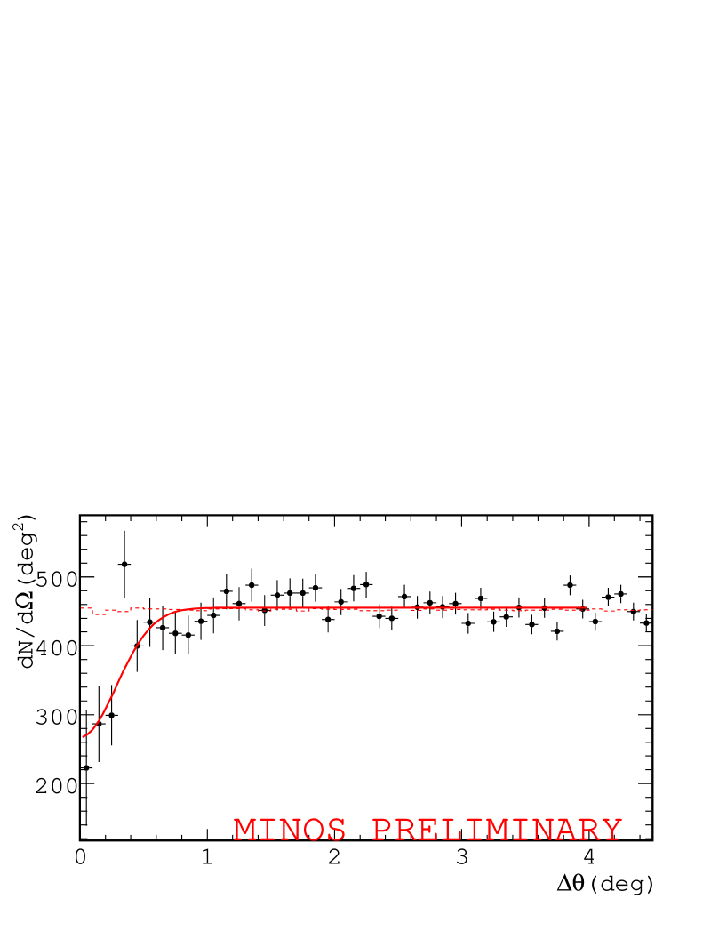
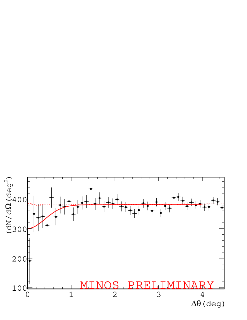
Figure 1: The differential muon flux with respect to displacement from the moon’s (l), and sun’s (r) location, binned in $0.1{{}^{o}}$. The dashed curve is the calculated background, while the solid curve is the best fit from eq. 1.

The one dimensional space angle separation was found using the Haversine formula, published in Sky and Telescope [Sinnott:1984]. The muons were binned in $S_{bin}=0.10^{\circ}$ increments, and since radial distance from the center of the celestial body is measured over a two dimensional projection, the bin solid angle of bin (i) increases when moving out from the center as $\Delta\Omega_{i}=(2i-1)*S_{bin}\pi$. Weighting the number of events in each bin by the reciprocal of the area resulted in the distribution $N_{i}/\Delta\Omega_{i}$, the differential muon density. The $\Delta\theta$ distribution is shown in Fig. 1 (l); from the sun, Fig. 1 (r), with statistical error bars displayed. There is a very clear deviation from a flat distribution in both plots as $\theta\rightarrow 0$, and that deviation is attributed to muons blocked by the moon and sun, respectively. The background was calculated using the method described in Sec. 2. As expected, the backgrounds are nearly flat, with a fit value of $\chi^{2}/ndf=0.12/39$ for the moon and $\chi^{2}/ndf=0.27/39$ for the sun . This Monte Carlo is consistent with the premise of a sourceless cosmic ray sky. The significance of the shadow can be found by fitting to the distribution a function of the form [4]:

$$\frac{\Delta N_{\mu}}{\Delta\Omega}=\lambda(1-(R_{m}^{2}/\sigma^{2})e^{-\theta^{2}/2\sigma^{2}})$$ (1)

where $\lambda$ is the average differential muon flux, $\sigma$ accounts for smearing from detector resolution, multiple coulomb scattering and geomagnetic deflection, and $R_{m}=0.26^{\circ}$, the angular radius of the moon. A fit to eq. 1 yields $\chi^{2}/ndf=37.9/38$, an improvement of 16.4 over the liner fit ($\chi^{2}/ndf=54.3/39$), with parameters $\lambda=483.9\pm 3.1$ and $\sigma=0.34^{\circ}\pm 0.07^{\circ}$. The change in $\chi^{2}$ over 38 degrees of freedom for the moon corresponds to a $10^{-}4$ chance probability. The improvement of $\chi^{2}$ probability for the sun corresponds to a $10^{-3}$ chance probability. These results are summarized in Table 1.

Since the tracks of dimuon events, muons that are induced by the same cosmic ray primary, are nearly parallel when they are created, they can be used to find the MINOS Point Spread Function. To quantify the absolute pointing of the Far Detector, the MINOS Point Spread Function will be used to find the two dimensional contours of the most significant muon deficit caused by the moon. This analysis is not complete at the time of this writing, however, so in its stead a simple approximation was used on the one dimensional moon shadow to place an quantify the pointing of the detector. A significant shadow pointing to the apparent location of the moon was found using a one dimensional space angle separation, a convolution of $\Delta RA,\Delta Dec$. Since the moon’s radius is $0.26^{\circ}$, we can approximate the absolute pointing of the detector as $0.3^{\circ}\pm 0.05^{\circ}$, with the error given by one half the bin width in theta. This analysis assumes that the pointing is reliable to begin with, so more precise analysis is still to be performed.

4 Charge-Separated Analysis

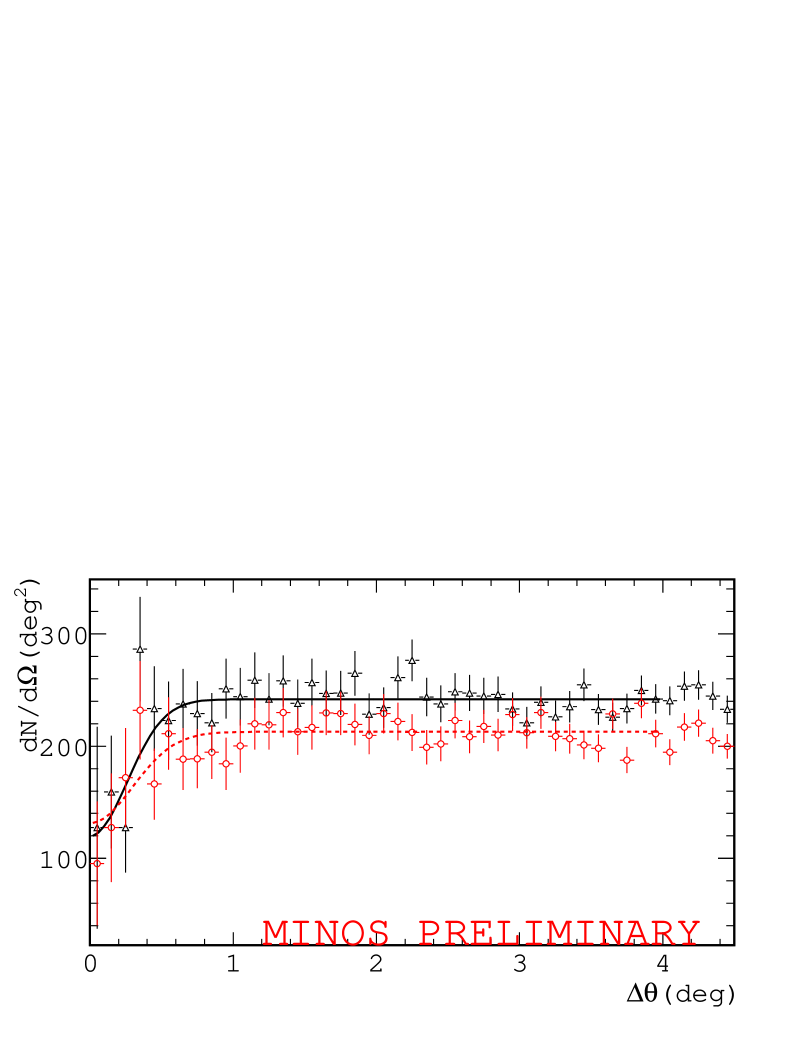
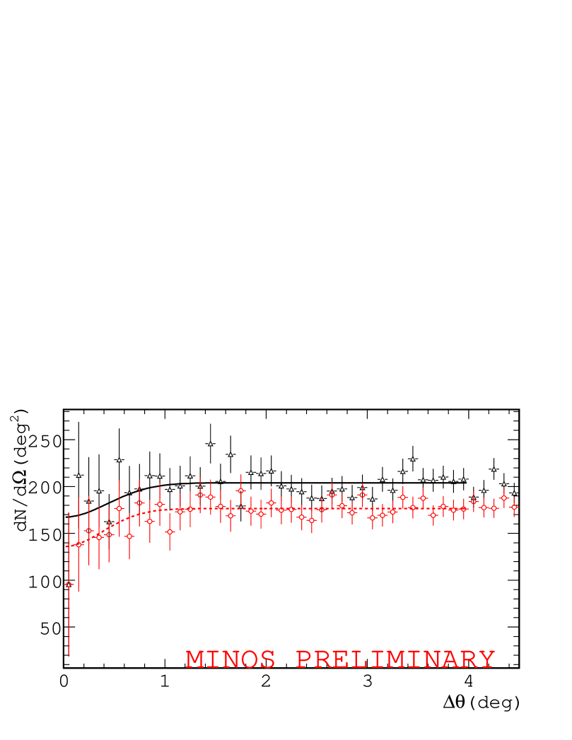
Figure 2: The differential muon flux with respect to displacement from the moon’s location (l), and sun’s location (r), binned in 0.1^o increments for $\mu^{+}$ (open circles) and $\mu^{-}$, (open triangles). The solid curve is the best fit from eq. 1 for $\mu^{+}$; the dashed curve is for $\mu^{-}$. The fit results are in Table 1.

For the charge separated sample, a further cut was required to exclude events with low confidence charge sign determination. The curvature of the track is used to determine the momentum and charge of the particle, so this cut was charge over momentum divided by the error in the determination of charge over momentum ($\frac{q/p}{\sigma_{q/p}}>2.2$) [Adamson:2007vt]. There are 2.7 million positively charged and 1.9 million negatively charged muon in this sample. An analysis similar to what is described in Sec. 3 was performed on the charge separated muon sample. The charge separated moon shadow plots can be seen in Fig. 2 (l), and the sun shadow plots are shown in Fig. 2 (r). The Gaussian hypothesis gives very little improvement over the flat hypothesis, suggesting that the shadow of the moon or sun has not been seen for the charge separated sample. The strong cut $\frac{q/p}{\sigma_{q/p}}$ reduces the statistics by over four times, from 20 to 4.6 million, eliminating an observable deficit in the direction of either sun or moon. This cut does give a charge ratio of 1.3 for both sun and moon distribution, which is consistent with the published MINOS result. This analysis has provided a flat distribution in the region approaching the moon, so given more statistics a significant shadow should be observed.

Distribution	$\Delta\chi^{2}$	prob.	$\lambda$	$\sigma$
moon-total	54.3-37.9 = 16.4	$10^{-4}$	$483.9\pm 3.1$	$0.34\pm 0.07$
moon-$\mu^{+}$	25.4 - 25.3= 0.1	N/A	$56.7\pm 1.4$	$N/A$
moon-$\mu^{-}$	17.4-16.0 = 1.4	N/A	$43.2\pm 1.2$	$N/A$
sun-total	48.5 - 40.3 = 8.2	$10^{-3}$	$397.4\pm 2.8$	$0.399\pm 0.09$
sun-$\mu^{+}$	23.23 -23.23 = 0	N/A	$48.2\pm 19.72$	$N/A$
sun-$\mu^{-}$	26.68 - 26.68 = 0	N/A	$36\pm 1.3$	$N/A$

Table 1: Significance for the shadowing observed in each distribution, with $\Delta\chi^{2}\equiv\chi_{line}^{2}-\chi_{gaus}^{2}$

5 Conclusions

Using 20.17 million muons accumulated over 1194 live-days, the MINOS Far Detector has observed the cosmic ray shadow of the moon with a high significance. Despite the inherent fragility of the one-dimensional moon shadow measurement (there were only nine events in the bin nearest to the moon), the null hypothesis of the muon deficit in the area near to the apparent location of the moon has a probability of $10^{-}4$.The cosmic ray shadow of the sun over the same time period has a chance probability of $10^{-3}$The shadow of the moon was used to approximate both the effective angular resolution of the detector, $0.34^{\circ}\pm 0.07^{\circ}$, and the absolute pointing of the detector, $0.30^{\circ}\pm 0.05^{\circ}$. In agreement with the expectation, no significant difference was found in the shadowing effects for either population, save for the charge ratio.

6 Acknowledgments

This work was supported by the U.S. Department of Energy and the University of Minnesota. Special thanks to the mine crew in Soudan for their tireless effort keeps the detector up and running.

References

- [1] D. E. Alexandreas et al. Observation of shadowing of ultrahigh-energy cosmic rays by the moon and the sun. Phys. Rev., D43:1735–1738, 1991.
- [2] A. Borione et al. Observation of the shadows of the moon and sun using 100- tev cosmic rays. Phys. Rev., D49:1171–1177, 1994.
- [3] M. Amenomori et al. Cosmic ray deficit from the directions of the moon and the sun detected with the tibet air shower array. Phys. Rev., D47:2675–2681, 1993.
- [4] J. H. Cobb et al. The observation of a shadow of the moon in the underground muon flux in the soudan 2 detector. Phys. Rev., D61:092002, 2000.
- [5] M. Ambrosio et al. Observation of the shadowing of cosmic rays by the moon using a deep underground detector. Phys. Rev., D59:012003, 1999.
- [6] M. Ambrosio et al. Moon and sun shadowing effect in the macro detector. Astropart. Phys., 20:145–156, 2003.
- [7] P. Achard et al. Measurement of the shadowing of high-energy cosmic rays by the moon: A search for tev-energy antiprotons. Astropart. Phys., 23:411–434, 2005.
- [8] S.L. Mufson. Measurement of the atmospheric muon charge ratio at tev energies with minos. In International Cosmic Ray Conference (these proceedings), 2007.
- [9] E.W. Grashorn. Observation of seasonal variations with the minos far detector. In International Cosmic Ray Conference (these proceedings), 2007.
- [10] J.D. Giorgini, D.K. Yeomans, A.B. Chamberlin, P.W. Chodas, R.A. Jacobson, M.S. Keesey, J.H. Lieske, S.J. Ostro, E.M. Standish, and R.N. Wimberly. Jpl’s on-line solar system data service. Bulletin of the American Astronomical Society, 28(3):1158, 1996.