Unit Rectangle Visibility Graphs

Abstract

Over the past twenty years, rectangle visibility graphs have generated considerable interest, in part due to their applicability to VLSI chip design. Here we study unit rectangle visibility graphs, with fixed dimension restrictions more closely modeling the constrained dimensions of gates and other circuit components in computer chip applications. A graph $G$ is a unit rectangle visibility graph (URVG) if its vertices can be represented by closed unit squares in the plane with sides parallel to the axes and pairwise disjoint interiors, in such a way that two vertices are adjacent if and only if there is a non-degenerate horizontal or vertical band of visibility joining the two rectangles. Our results include necessary and sufficient conditions for $K_{n}$, $K_{m,n}$, and trees to be URVGs, as well as a number of general edge bounds.

1 Introduction

Over the past twenty years the difficulty of VLSI chip design and layout problems has motivated the study of bar visibility graphs (BVGs) [3, 5, 6, 11, 12, 16, 17] and their two-dimensional counterparts, rectangle visibility graphs (RVGs) [1, 4, 9, 13, 14, 15]. In these constructions, horizontal bars or rectangles in the plane model gates or other chip components, and edges are modeled by vertical visibilities between bars, or by vertical and horizontal visibilities between rectangles. The two visibility directions in RVGs provide a model for two-layer chips with wires running horizontally on one layer and vertically on the other. The dimensions of bars and rectangles in BVGs and RVGs may vary arbitrarily, but chip components typically have restricted area and aspect ratios. In order to more closely model the restricted dimensions of chip components, Dean and Veytsel [5] studied unit bar visibility graphs (UBVGs), in which all bars have equal length. A related model, using boxes in 3-space, was studied in [2, 8]. In this paper we study the similarly restricted class of RVGs, unit rectangle visibility graphs (URVGs), in which all rectangles are unit squares.

In Section 2 we give definitions and basic properties that we use throughout the paper. In Section 3 we characterize the complete graphs that are URVGs. In Section 4 we characterize URVG trees, and we show that any graph with linear arboricity 2 is a URVG. In section 5 we characterize which complete bipartite graphs are URVGs or subgraphs of URVGs. In section 6 we give edge bound results for URVGs as well as examples that show these bounds are tight up to constant coefficients. We provide edge bounds for depth-$s$ UBV and URV trees, bipartite URVGs, and arbitrary URVGs. In Section 7 we state two open problems on URVGs.

2 Definitions and Basic Properties

2.1 Definition.

A graph $G$ is a unit rectangle visibility graph or URVG if its vertices can be represented by closed unit squares in the plane with sides parallel to the axes and pairwise disjoint interiors, in such a way that two vertices are adjacent if and only if there is an unobstructed non-degenerate (positive width) horizontal or vertical band of visibility joining the two rectangles.

We denote the square in the URV layout corresponding to a vertex $v$ by $S_{v}$. We identify the position of the square $S_{v}$ in a URV layout by its bottom-left corner coordinates $(x_{v},y_{v})$. We define $X_{v}$ to be the line segment given by the intersection of the line $x=x_{v}$ with the square $S_{v}$, and $Y_{v}$ to be the line segment given by the intersection of the line $y=y_{v}$ with the square $S_{v}$.

Two squares $S_{v}$ and $S_{w}$ are called flush if $x_{v}=x_{w}$ or $y_{v}=y_{w}$ (this does not preclude other squares obstructing visibility between $S_{v}$ and $S_{w}$). In Fig. 1, squares $S_{2}$ and $S_{3}$ are collinear but not flush, and squares $S_{1}$ and $S_{2}$ are flush, as are squares $S_{1}$, $S_{5}$, and $S_{6}$.

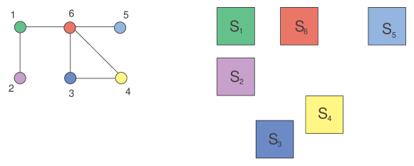
Figure 1: A graph with a URV layout.

2.2 Definition.

A graph $G$ is a weak unit rectangle visibility graph if its vertices can be represented by closed unit squares in the plane with sides parallel to the axes and pairwise disjoint interiors, in such a way that whenever two vertices are adjacent there is an unobstructed non-degenerate, horizontal or vertical band of visibility joining the two rectangles. Equivalently, $G$ is a weak URVG if it is a subgraph of a URVG.

An example of a graph with a weak URV layout is given in Fig. 2. (There is a band of visibility between squares $S_{3}$ and $S_{4}$ but no edge $\{3,4\}$.) We conclude this section with a straightforward but useful proposition.

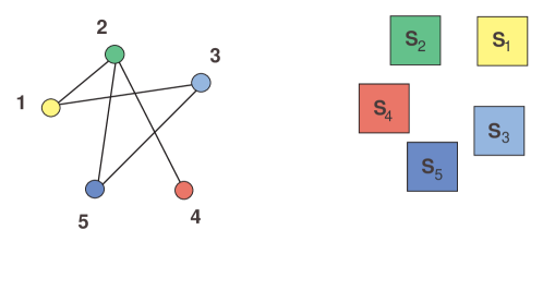
Figure 2: A graph with a weak URV layout.

2.3 Proposition.

If $G$ has a URVG layout $L$, let $G_{X}$ and $G_{Y}$ denote the graphs induced by the horizontal and vertical visibilities of $L$. $G_{X}$ and $G_{Y}$ are UBVGs with bars given by $\{X_{v}|v\in G\}$ and $\{Y_{v}|v\in G\}$, and $G=G_{X}\bigcup G_{Y}$.

Fig. 3 illustrates the decomposition of a URV layout into horizontal and vertical UBV layouts.

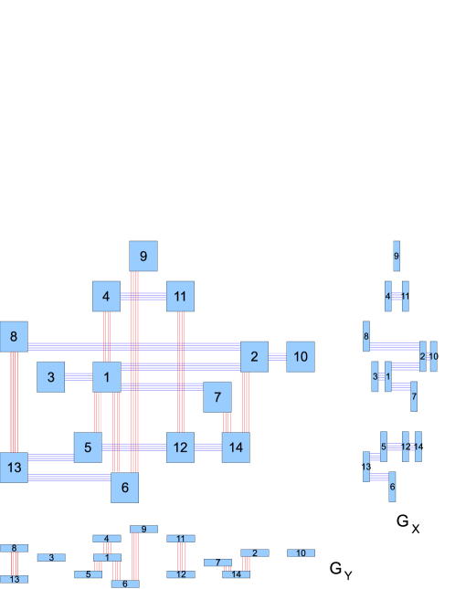
Figure 3: URV layout and corresponding UBV layouts for $G_{X}$ and $G_{Y}$.

3 Cycles and Complete Graphs

In this section we characterize the cycles and complete graphs that are URVGs.

3.1 Proposition.

The $n$-cycle $C_{n}$ is a URVG.

See Fig. 4 for a layout of $C_{n}$.

Figure 4: A layout of the $n$-cycle $C_{n}$.

The following theorem of Erdös and Szekeres [7] will be used in characterizing which graphs are URVGs.

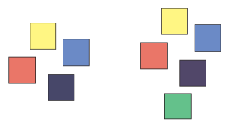
Figure 5: URV layouts of $K_{4}$ and of $K_{5}$ minus one edge.

3.2 Theorem.

(Erdös and Szekeres [7]) For $n\geq 0$, every sequence $a_{1},a_{2},$ …, $a_{n^{2}+1}$ of $n^{2}+1$ terms contains a monotonic subsequence of $n+1$ terms.

3.3 Theorem.

$K_{n}$ is a URVG if and only if $n\leq 4$.

Proof.

We first note that since all edges are present in a complete graph, any URV layout of $K_{n}$ gives a URV layout of $K_{m}$ for all $m\leq n$. Thus it suffices to prove that $K_{4}$ is a URVG and $K_{5}$ is not a URVG. Fig. 5 gives a URV layout of $K_{4}$. To show that $K_{5}$ is not a URVG, we first observe that if squares $S_{1},S_{2},S_{3}$ give a URV layout of $K_{3}$ with $x_{1}\leq x_{2}\leq x_{3}$ then $(y_{1},y_{2},y_{3})$ must be non-monotonic. This follows since if the sequence $(y_{1},y_{2},y_{3})$ is monotonic, then $S_{2}$ blocks $S_{3}$ from seeing $S_{1}$. Now suppose we have a URV layout of five squares. By relabeling if necessary, we may assume that $x_{1}\leq x_{2}\leq x_{3}\leq x_{4}\leq x_{5}$. Now consider the sequence of $y$-coordinates. By Theorem 3.2 this sequence has a monotonic subsequence of length 3, say $(y_{i_{1}},y_{i_{2}},y_{i_{3}}).$ Thus the squares $S_{i_{1}},S_{i_{2}},S_{i_{3}}$ cannot be a layout of $K_{3}$, and the five squares cannot be a layout of $K_{5}$. ∎

3.4 Corollary.

Any graph G that contains $K_{5}$ as a subgraph is not a URVG.

Remark.

Proposition 2.3 states that every URVG is the union of two UBVGs. Fig. 6 gives a decomposition of $K_{5}$ into the union of two UBVGs, so the converse of Proposition 2.3 is false.

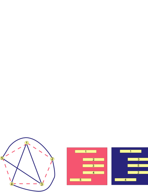
Figure 6: $K_{5}$ is the union of two UBVGs.

4 Trees, Caterpillars, and Arboricity 2

In this section we characterize the trees that are URVGs. We begin with a simple necessary degree condition.

4.1 Theorem.

If $v$ is a vertex of a URVG $G$ with degree $\geq 7$, then $v$ lies on a cycle.

Proof.

Suppose $G$ is a URVG having a vertex $v$ with degree $\geq 7$. Let $G_{X}$ and $G_{Y}$ be the UBVGs induced by the horizontal and vertical visibilities of a URV layout of $G$, as described in Proposition 2.3. Since $deg(v)\geq 7$, it follows from the Pigeonhole Principle that $deg(v)\geq 4$ in $G_{X}$ or $G_{Y}$. Without loss of generality, assume that $deg(v)\geq 4$ in $G_{X}$. In ([5], Corollary 1.7) it is shown that any vertex in a UBVG with degree $\geq 4$ lies on a cycle. Since $G_{X}$ is a subgraph of $G$, it follows that $v$ lies on a cycle in $G$. ∎

4.2 Corollary.

A URVG tree T has maximum degree $\leq~{}6$.

4.3 Definition.

A caterpillar is a tree in which all vertices with degree greater than 1 lie on a single path. Such a path is called a spine of the caterpillar if it has maximal length. A subdivided caterpillar is a caterpillar in which each edge may be replaced by a path of arbitrary length. A leg of a caterpillar or subdivided caterpillar is a path having one endpoint on the spine and the other a degree-1 vertex. See Fig. 7.

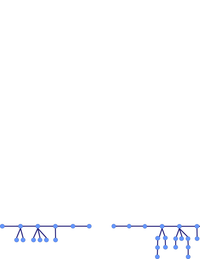
Figure 7: A caterpillar and a subdivided caterpillar.

The following theorem of Dean and Veytsel [5] characterizes the trees that are UBVGs.

4.4 Theorem.

(Dean and Veytsel [5], Theorem 3.5) A tree is a UBVG if and only if it is a subdivided caterpillar with maximum degree 3.

It follows from Proposition 2.3 that if a tree is a URVG, it is the union of two subdivided caterpillar forests, each with maximum degree 3. Although in general it is not true that the union of two UBVGs is a URVG, as illustrated in Fig. 6, we show that a tree $T$ is a URVG if and only if its horizontal and vertical UBVG subgraphs, $T_{X}$ and $T_{Y}$, are UBV forests.

4.5 Theorem.

A tree $T$ is a URVG if and only if it is the union of two subdivided caterpillar forests, each with maximum degree 3.

Proof.

Necessity follows from Theorem 4.4 and Proposition 2.3. For sufficiency, we give an algorithm to construct a URVG layout:

INPUT: A partition of a tree $T$ into two caterpillar forests $F_{1}$ and $F_{2}$, each having maximum degree 3.

OUTPUT: A URVG layout of $T$ with $T_{X}=F_{1}$ and $T_{Y}=F_{2}$.

Choose an arbitrary root $r$ for $T$ and give $T$ a breadth-first numbering, $v_{1},\ldots,v_{n}$, starting with $r=v_{1}$. For each $i$, let $S_{i}$ denote the square in the URVG layout representing $v_{i}$, and let $(x_{i},y_{i})$ be the coordinates of the lower left corner of $S_{i}$. The algorithm places square $S_{1}$ arbitrarily, and then, for $i=1,\ldots,n-1$, it places squares representing the children of vertex $v_{i}$. For each $i=1,\ldots,n-1$, at the point in the algorithm at which we have placed a square for $v_{i}$ and squares for all its children, but no higher-numbered squares, the following set of invariants is maintained.

Algorithm Invariants:

1. A leg edge in $F_{1}$ corresponds to a horizontal flush visibility in the layout.

2. A leg edge in $F_{2}$ corresponds to a vertical flush visibility in the layout.

3. A spine edge in $F_{1}$ corresponds to a horizontal protruding (i.e., not flush) visibility in the layout.

4. A spine edge in $F_{2}$ corresponds to a vertical protruding visibility in the layout.

5. If a vertex $v_{j}$ has parent $v_{i}$ in the breadth-first numbering, where $i<j$, then at the point when the square $S_{j}$ is placed, it sees no square other than $S_{i}$.

We observe that if $S_{i}$ is a square in the layout corresponding to vertex $v_{i}$, then $v_{i}$ may have either at most two incident leg edges in $F_{1}$, or at most one incident leg edge and two incident spine edges in $F_{1}$. In the former case the algorithm places the squares for the two leg neighbors of $S_{i}$ flush with it on opposite sides. In the latter case, the square for the leg neighbor is placed flush on one side of $S_{i}$, and both squares for the spine neighbors are placed on the opposite side of $S_{i}$, protruding so that they both see $S_{i}$ but not one another. A similar statement holds for the neighbors of $v_{i}$ in $F_{2}$; see Fig. 8. The algorithm chooses the exact placement of each square so as not to introduce unwanted visibilities with other squares that have already been placed.

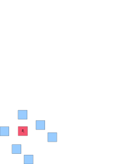
Figure 8: Placement of neighbor squares in a tree layout.

Algorithm to create a URVG layout of the tree $T$:

1. Let $i=1$, and arbitrarily place square $S_{1}$ representing $v_{1}$. Define $x_{m}$ to be the smallest $x$-coordinate of any square that has been placed in the layout and $x_{M}$ to be the largest $x$-coordinate of any square that has been placed in the layout. Similarly, define $y_{m}$ and $y_{M}$ to be the smallest and largest $y$-coordinates of any squares that have been placed in the layout.

2. Place squares representing the children of $v_{1}$ as follows, maintaining the invariants:

   • There are at most two leg edges of $F_{1}$ incident with $v_{1}$. Place squares representing the endpoints of these edges, if they exist, at position $(x_{1}-2,y_{1})$ for the first (in breadth-first order) and $(x_{1}+2,y_{1})$ for the second. For leg edges of $F_{2}$ incident with $v_{1}$, place the squares at $(x_{1},y_{1}-2)$ and $(x_{1},y_{1}+2)$.

   • If $v_{1}$ is incident to any spine edges in $F_{1}$, then it is incident to at most two such edges, and it is incident to at most one leg edge of $F_{1}$, already placed at $(x_{1}-2,y_{1})$. Place squares representing the endpoints of the spine edges, if they exist, at $(x_{1}+2,y_{1}+2/3)$ and $(x_{1}+4,y_{1}-2/3)$, in breadth-first order. For spine edges of $F_{2}$ incident with $v_{1}$, place the squares at $(x_{1}+2/3,y_{1}+2)$ and $(x_{1}-2/3,y_{1}+4)$.

3. Let $i=i+1$. Square $S_{i}$ has been placed as a child of its parent square $S_{p}$, where $1\leq p<i$. If $i=n$, the layout is complete, since $v_{n}$ has no children. Otherwise, we place squares for each child $v_{j}$ of $v_{i}$ as follows:

   • Leg edges to children of $v_{i}$: If $v_{i}$ has a leg edge $v_{i}$–$v_{j}$ in $F_{1}$, incident to a child $v_{j}$, the placement of $S_{j}$ depends on the relative placements of $S_{i}$ and its parent square $S_{p}$. If $v_{i}$–$v_{p}$ is also an edge (leg or spine) of $F_{1}$, assume without loss of generality (since we can flip the existing layout horizontally or vertically if necessary) that its square was placed to the left of $S_{i}$. Then we place the square $S_{j}$ to the right of $S_{i}$, at position $(x_{M}+2,y_{i})$. Otherwise we place the (at most two) leg edges of $F_{i}$ from $v_{i}$ to its children, in breadth-first order, at positions $(x_{m}-2,y_{i})$ and $(x_{M}+2,y_{i})$. We place squares representing the endpoints of (at most two) leg edges of $F_{2}$ from $v_{i}$ to its children in an analogous manner, using positions $(x_{i},y_{m}-2)$ and $(x_{i},y_{M}+2)$. The values of $x_{m}$, $x_{M}$, $y_{m}$, and $y_{M}$ are updated after the placement of each square.

   • Spine edges to children of $v_{i}$: If $v_{i}$ has a spine edge $v_{i}$–$v_{j}$ in $F_{1}$, incident to a child $v_{j}$, the placement of $S_{j}$ depends on the relative placements of $S_{i}$ and its parent square $S_{p}$. If $v_{p}$–$v_{i}$ is a leg edge of $F_{1}$, then $S_{p}$ is a horizontal, flush neighbor of $S_{i}$; assume without loss of generality that $S_{p}$ is flush neighbor lying to the right of $S_{i}$. If $v_{p}$–$v_{i}$ is a spine edge of $F_{1}$, then $S_{p}$ is a horizontal, protruding neighbor of $S_{i}$. Without loss of generality, we assume that $S_{p}$ lies to the left of $S_{i}$ and is a downward protruding neighbor of $S_{i}$.

     We wish to place $S_{j}$ as an upward protruding neighbor of $S_{i}$, also lying to the left of $S_{i}$ (on the side opposite of $S_{p}$ if $v_{p}$ is a leg neighbor of $v_{i}$ in $F_{1}$, and on the same side if $v_{p}$ is a spine neighbor of $v_{i}$ in $F_{1}$). Invariant 5 guarantees that a horizontal line through the upper edge of $S_{i}$ intersects the interiors of no other squares in the layout. We replace that line with a horizontal band of height one to create room for an upward protruding neighbor of $S_{i}$; see Fig. 9. If $x_{m}$ is the smallest $x$-coordinate in the current layout, then the coordinates of $S_{j}$ are $(x_{m}-2,y_{i}+2/3)$, and the invariants are maintained. The values of $x_{m}$, $x_{M}$, $y_{m}$, and $y_{M}$ are updated after placement.

     If $v_{p}$–$v_{i}$ is not a spine edge of $F_{1}$, then place the square for the first spine neighbor in $F_{1}$ to the left of $S_{i}$ as described above. To place a square for a second spine neighbor of $v_{i}$ in $F_{1}$, we replace the line through the lower edge of $S_{i}$ with a horizontal band of height one, creating room to place the square at position $(x_{m}-2,y_{i}-2/3)$. The values of $x_{m},x_{M},y_{m}$, and $y_{M}$ are updated after placement.

     We place squares representing the endpoints of (at most two) spine edges of $F_{2}$ from $v_{i}$ to its children in an analogous manner, using positions $(x_{i}-2/3,y_{m}-2)$ and $(x_{i}+2/3,y_{m}-2)$.

4. At this point squares representing all the children of $v_{i}$ have been placed. Return to step 3.

∎

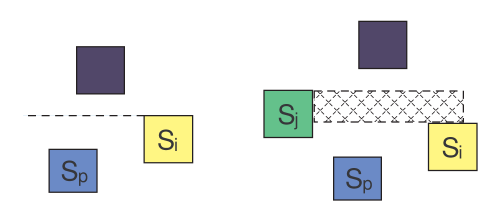
Figure 9: Making room for a child square $S_{j}$ of $S_{i}$.

A comparable result holds for general graphs, if we require a decomposition into two forests of paths, rather than into subdivided caterpillar forests with maximum degree 3. The linear arboricity of a graph $G$ is the minimum number of linear forests whose union is $G$. Similarly the caterpillar arboricity of $G$ is the minimum number of caterpillar forests whose union is $G$. It is shown in ([1], Theorem 5) that, if $G$ has caterpillar arboricity 2, then it is an RVG. The proof is constructive: each caterpillar forest is represented as an interval graph, one along the $x$-axis and the other along the $y$-axis. The Cartesian product of horizontal and vertical intervals corresponding to the same vertex is a rectangle in the plane, and the resulting set of rectangles is an RVG representation of $G$. If it happens that both caterpillar forests are actually linear forests, then the intervals can all have equal length, making $G$ a URVG; an example is shown in Fig. 10. Hence the following result follows immediately.

4.6 Theorem.

If $G$ has linear arboricity 2, then $G$ is a URVG.

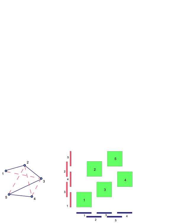
Figure 10: URV layout of a graph with linear arboricity 2.

The next result states that, in contrast to Theorem 4.5, every tree is a weak UBVG. See Fig. 11 for a sample layout.

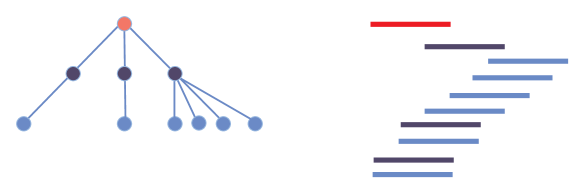
Figure 11: Weak UBV layout of a tree.

4.7 Theorem.

Every tree is a weak UBVG, and hence a weak URVG.

Proof.

We prove this by providing an algorithm to construct a weak UBV layout. Let $T$ be a tree. Choose an arbitrary root $r$, and give $T$ a breadth-first numbering starting with $r=0$. We specify the position of a bar corresponding to vertex $v$ by the coordinates of its left endpoint $(v_{x},v_{y})$. We begin by placing the bar corresponding to $r$ at position $(0,0)$. If $r$ has $k_{0}$ children, place the bar for child $i$ of $r$ at position $(1-i/k_{0},-i)$. Next we will place the vertices on level two. If parent $p$ has $k_{p}$ children insert a horizontal band of height $k_{p}$ below the bar corresponding to $p$ in the layout. Child $i$ of parent $p$ should then be placed at position $(x_{p}+1-i/k_{p},y_{p}-i)$. Continue in this manner to place the children on the remaining levels. ∎

5 Complete Bipartite Graphs

In this section we establish which complete bipartite graphs are URVGs, and which are weak URVGs. Throughout, we always write $K_{m,n}$ with $m\leq n$, and we denote by $V_{m}$ and $V_{n}$ the two partite sets of $K_{m,n}$.

5.1 Theorem.

The complete bipartite graph $K_{m,n}$, $m\leq n$, is a URVG if $m\leq 2$ and $n\leq 6$, or $m=3$ and $n\leq 4$. $K_{m,n}$ is a weak URVG if $m\leq 2$ (and $n$ is arbitrary), or $m\leq 3$ and $n\leq 4$.

Proof.

URV layouts of $K_{1,6}$, $K_{2,6}$, and $K_{3,4}$ are shown in Fig. 12. A weak URV layout of $K_{2,n}$ is shown in Fig. 13. Layouts for smaller values of $n$ are obtained by deleting squares from these layouts. ∎

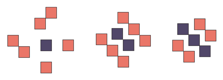
Figure 12: URV Layouts of $K_{1,6}$, $K_{2,6}$, and $K_{3,4}$.

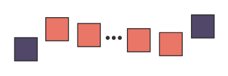
Figure 13: A weak URV layout of $K_{2,n}$.

The results of the remainder of this section prove that the conditions of Theorem 5.1 are also necessary.

Given a URV layout of $K_{m,n}$, we write $K_{X}$ and $K_{Y}$ for $(K_{m,n})_{X}$ and $(K_{m,n})_{Y}$. We call a cycle in a plane graph empty if it bounds a finite face. As noted in ([5], Proposition 1.10), the layout of an empty $n$-cycle $C$ in a UBVG corresponds to a vertical line $\ell_{C}$ joining the interiors of the top and bottom cycle bars, such that each of the other $n-2$ ‘intermediate’ bars of $C$ has its left or right endpoint on $\ell_{C}$. See Fig. 14. We call a UBV layout of an empty cycle one-sided if all the intermediate bars lie on the same side of $\ell_{C}$ and two-sided otherwise.

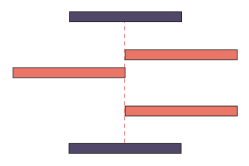
Figure 14: Two-sided UBV layout of an empty cycle.

5.2 Lemma.

If $C$ is a cycle in a UBVG, then in the plane embedding induced by the corresponding UBV layout, every edge of $C$ lies on an empty cycle.

Figure 15: A cycle whose edges do not lie on an empty cycle.

Proof.

It follows from the characterization of BVGs in ([17],Theorem 4) and ([16], Theorem 5) that the plane embedding induced by a UBV layout has all cutpoints on the exterior face, but we must show that no 2-connected block incident with such a cutpoint lies in the interior of a finite face; see Fig. 15. We claim that the subgraph $G_{C}$ comprised of the vertices and edges lying on $C$ and in its interior is 2-connected. First, $C$ itself is a 2-connected graph. Next, let $b_{w}$ be a bar in the interior of $G_{C}$. The set comprised of the bars of $C$, together with vertical lines representing visibilities corresponding to the edges of $C$, contains a Jordan curve. Thus, if we pass a vertical line through $b_{w}$, it will induce a path of visibilities containing $b_{w}$ from one vertex $u$ of $C$ to another vertex $v$ of $C$. Hence, every vertex in $G_{C}$ lies on a path joining two vertices of $C$. Therefore $G_{C}$ is 2-connected, and so its internal faces are bounded by empty cycles. ∎

5.3 Lemma.

If there is a URV layout of $K_{m,n}$ with an empty cycle $C$ in $K_{Y}$, then $C$ is a 4-cycle, $m=2$, and the maximum degree of any vertex in $K_{Y}$ is 3. Furthermore,

1. If $C$ is one-sided, then $2\leq n\leq 3$;

2. If $C$ is two-sided, then $2\leq n\leq 4$.

An analogous result holds when $C$ is in $K_{X}$.

Proof.

First we note that $C$ has at most two left-intermediate and two right-intermediate bars: if $C$ has, say, three or more left-intermediate bars, let $Y_{p}$ be the third-highest one of these. Then $p$ and $t$ are in different partite sets, but $S_{p}$ cannot see $S_{t}$. Next note that there cannot be both two left-intermediate bars and two right-intermediate bars, because then $t$ and $b$ would be in different partite sets, but $S_{t}$ could not see $S_{b}$. So $C$ is a 4-cycle, and either $C$ has one left-intermediate and one right-intermediate bar or, without loss of generality, two left-intermediate bars and no right-intermediate bars.

Suppose next that $C$ has two left-intermediate bars with $Y_{u}$ the higher of the two. Without loss of generality, assume that $x_{t}\leq x_{b}$, as illustrated in Fig. 16(a). Then the only way there can be additional squares is if $x_{t}<x_{b}$, and a square $S_{p}$ is placed with $x_{t}+1\leq x_{p}<x_{b}$, so that $S_{p}$ sees $S_{u}$ horizontally and $S_{b}$ vertically. Furthermore at most one such square can be placed this way, thus $m=2$ and $2\leq n\leq 3$.

Lastly, assume $C$ has one left-intermediate and one right-intermediate bar. Then $t$ and $b$ are in the same partite set, and the intermediate bars prevent them from having any other common neighbors in the URV layout. Hence $m=2$. It is possible to place at most two more squares in the same partite set as $t$ and $b$, as illustrated in Fig. 16(b), so that $2\leq n\leq 4$. Furthermore, each of these squares must see one intermediate square horizontally and the other vertically, so that the maximum degree of any vertex in $K_{Y}$ is 3. ∎

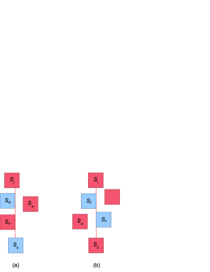
Figure 16: The two cases of Lemma 5.3.

5.4 Lemma.

If $n\geq 7$, then $K_{m,n}$ is not a URVG.

Proof.

We assume $K_{m,n}$ has a URV layout and obtain a contradiction. Since $n\geq 7$, there is a vertex $s$ in, say, $K_{V}$, that has vertical degree $\geq 4$. By ([5], Corollary 1.7) the vertex $s$ lies on a cycle in $K_{V}$, and so by Lemma 5.2, $s$ lies on an empty cycle. This contradicts the degree conditions of Lemma 5.3. ∎

5.5 Theorem.

If $m,n\geq 4$, or $m\geq 3$ and $n\geq 5$, then $K_{m,n}$ is not a weak URVG.

Proof.

Let $m,n\geq 4$ or $m\geq 3,n\geq 5$, and suppose that $L$ is a weak URV layout of $K_{m,n}$. If necessary, we modify the layout slightly so that it becomes noncollinear without losing any visibilities. By a monotonic set of squares we mean a set of squares whose set of $y$ coordinates forms a monotonic sequence when listed in increasing order of the $x$ coordinates. The conditions on $m,n$ imply that there are eight or more vertices, so by Theorem 3.2 there is a monotonic set of three squares in the layout $L$. We assume without loss of generality that this set is monotonically increasing. We consider two cases depending on whether or not such a sequence exists with all elements in the same partite set.

Case 1: There is an increasing set of three squares $\{S_{1},S_{2},S_{3}\}\subseteq V^{\prime}=V_{m}$ or $V_{n}$. Let $V^{\prime\prime}=V(K_{m,n})\setminus V^{\prime}$, and assume without loss of generality the squares are labeled from left to right, $S_{1},S_{2},S_{3}$. Note that no square $S_{b}$ with $b\in V^{\prime\prime}$ can be part of a larger increasing sequence containing $S_{1},S_{2},S_{3}$, because then $S_{b}$ would be able to see at most two other squares in the sequence. For an element $b\in V^{\prime\prime}$, consider the 3-tuple of directions from which $S_{b}$ sees $S_{i},i=1,2,3$. For example, the 3-tuple $(N,N,W)$ signifies that $S_{b}$ is above $S_{1}$ and $S_{2}$, so sees them from the north, and is to the left of $S_{3}$, so sees it from the west. Because $S_{1},S_{2},S_{3}$ is an increasing sequence, a 3-tuple must have at least two consecutive repeated terms. The triples $(N,N,E)$, $(W,S,S)$, $(E,E,N)$, and $(S,W,W)$ are prohibited. The remaining possible 3-tuples are:

$$(N,N,N),(N,N,W),(N,N,S),(S,S,S),(E,S,S),(N,S,S),$$

$$(E,E,E),(E,E,S),(E,E,W),(W,W,W),(N,W,W),(E,W,W).$$

Since $S_{1},S_{2},S_{3}$ is increasing, if $S_{b}$ sees two squares from the north or east they must be $S_{1}$ and $S_{2}$, and if from the south or west they must be $S_{2}$ and $S_{3}$. Note that when $S_{b}$ sees two squares from the same direction, it blocks any other square from simultaneously seeing those two squares from that direction, so $|V^{\prime\prime}|\leq 4$.

We next show that, while $V^{\prime\prime}$ may have three or four elements, $V^{\prime}$ can have only three, so it is not the case that $m,n\geq 4$ or $m\geq 3$ and $n\geq 5$.

We label the four possible elements that $V^{\prime\prime}$ could have by $S_{n},S_{s},S_{e},$ $S_{w}$, to indicate the direction from which they each see more than one of $S_{1},S_{2},S_{3}$, as prescribed by the 3-tuples above. The following argument applies whether or not $S_{w}$ is present (indicated by [ ]), and by symmetry it applies if any three of the four are present. Consider the square $S_{2}$, which all four of these squares see in the directions prescribed by their subscripts. There are four disjoint regions of the plane composed of points not visible to $S_{2}$, located to the northwest, southwest, southeast, and northeast of $S_{2}$; see Fig. 17(a). Because $S_{n}$ sees both $S_{1}$ and $S_{2}$ from the north, and because $\{S_{1},S_{2},S_{3}\}$ is increasing, $S_{n}$ must intersect the region northwest of $S_{2}$. Similarly, [$S_{w}$ also intersects this region, while] $S_{s}$ and $S_{e}$ both intersect the region southeast of $S_{2}$. If there is an additional square $S_{4}\in V^{\prime}$ in the layout, it cannot intersect the region northwest of $S_{2}$, since then it cannot see either $S_{s}$ or $S_{e}$; likewise it cannot intersect the region southeast of $S_{2}$ since it must see $S_{n}$ [and $S_{w}$]. Assume without loss of generality that $S_{4}$ intersects the region northeast of $S_{2}$ (recall our assumption that the layout is noncollinear). Since both $S_{1},S_{2},S_{3}$ and $S_{1},S_{2},S_{4}$ are increasing sets, we relabel $S_{3}$ and $S_{4}$, if necessary, so that $S_{3}$ is further left than $S_{4}$. Now $S_{s}$ sees $S_{3}$ and $S_{4}$ from the south, so $S_{e}$ cannot see both these squares from the south. Hence $S_{e}$ must see the one that is further left, namely $S_{3}$, from the east, forcing $S_{3}$ to intersect the visibility corridor to the east of $S_{2}$. But this prevents $S_{4}$, which intersects the region northeast of $S_{2}$, and which is further right than $S_{3}$, from seeing $S_{s}$. This conclusion is reached whether or not $S_{w}$ is present, so by symmetry, we conclude that $V^{\prime}$ has at most three elements.

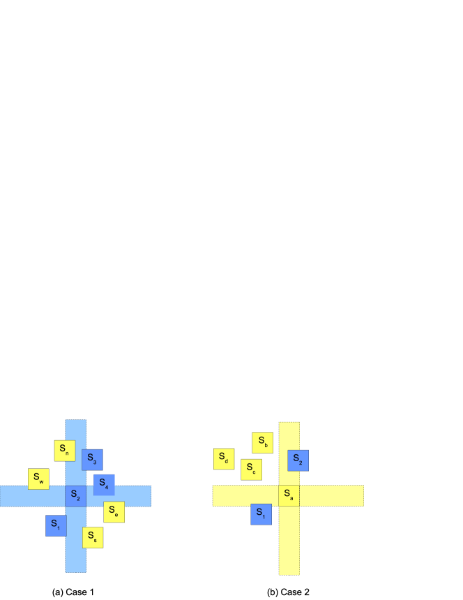
Figure 17: Positions of squares in proof of Theorem 5.5.

Case 2: There is no monotonic subsequence of length 3 or more with all elements in one of $V^{\prime},V^{\prime\prime}$. By Theorem 3.2, this can occur only if both $m$ and $n$ are $\leq 4$ so $m=n=4$. Again by Theorem 3.2, there is a strictly increasing subsequence of length 3 or more with two elements in $V^{\prime}$ and one element in $V^{\prime\prime}$. Note that the element of $V^{\prime\prime}$ in the increasing sequence of three must be the middle in order to see both of the other two, so we name these elements left to right, $S_{1},S_{a},S_{2}$. As in Case 1, consider the regions northwest, southwest, southeast, and northeast of the middle square, $S_{a}$. The square $S_{1}$ can intersect only the southwest region, and $S_{2}$ can intersect only the northeast region. No other element of $V^{\prime\prime}$ can intersect these two regions, because then it cannot see whichever of $S_{1}$ or $S_{2}$ intersects only the diagonally opposite region. Without loss of generality, assume that there is another square $S_{b}$ that intersects the region northwest of $S_{a}$. Then no element of $V^{\prime\prime}$ can intersect the southeast region, because it, together with $S_{a}$ and $S_{b}$, would form a monotonic set of length 3, contradicting the assumption of Case 2. Suppose there are three or more elements of $V^{\prime\prime}$ in the region northwest of $S_{a}$; see Fig. 17. Since none can have y-coordinates less than $S_{1}$’s and they can’t be monotonic, then some two out of the three form a monotonic set with $S_{1}$, giving a contradiction. Thus $V^{\prime\prime}$ has at most three elements. ∎

6 Edge Bounds

In this section we give several results bounding the number of edges of URVGs. First we use the characterizations of Theorems 4.4 and 4.5 to give tight upper bounds on the number of edges in a depth-$s$ UBV tree and in a depth-$s$ URV tree. Next we modify the methods used for RVGs in [9] and [4] to bound the number of edges in general URVGs and bipartite URVGs, respectively, and we give examples to show that these bounds have tight order.

Edge bounds for depth-$s$ trees

6.1 Theorem.

If $T$ is a rooted depth-$s$ tree that is a unit bar visibility graph, then $T$ has at most $s^{2}+2s$ edges.

Proof.

Throughout we use the result of Theorem 4.4, that a tree is a UBVG if and only if it is a subdivided caterpillar forest with maximum degree 3. Define $T_{B,s}$ to be the subdivided caterpillar whose spine has length $2s+1$, rooted at the center spine vertex, and with a leg at each vertex extending to depth $s$, as illustrated in Fig. 18. By Theorem 4.4, $T_{B,s}$ is a UBVG, and it’s easy to see that the number of edges of $T_{B,s}$ equals $3+5+\ldots+(2s+1)=\sum_{k=1}^{s}(2k+1)=s^{2}+2s$. If $T\neq T_{B,s}$ and $T$ is rooted at a spine vertex, then $T$ is a subtree of $T_{B,s}$. If $T\neq T_{B,s}$ and $T$ is not rooted at a spine vertex, suppose that $v$ is the spine vertex closest to the root $r$ of $T$, and that $v$ is a depth-$q$ vertex, where $1<q\leq s$. Then the subtree rooted at $v$ is a subtree of $T_{B,s-q}$ with no leg at $v$, so it has at most $(s-q)^{2}+2(s-q)-(s-q)$ $=s^{2}-2sq+q^{2}+s-q$ edges. The path from $v$ to $r$ adds another $q$ edges plus $s$ possible edges on a path from $r$ to depth $s$, for a total of at most $s^{2}+2s-2sq+q^{2}=(s-q)^{2}+2s<s^{2}+2s$ edges. ∎

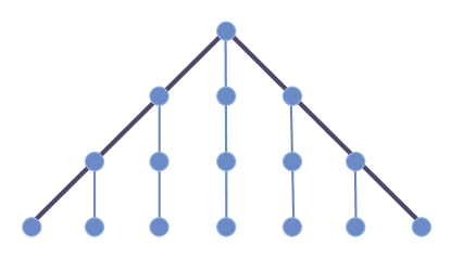
Figure 18: The depth-3 UBVG tree $T_{B,3}$.

6.2 Theorem.

Let $T$ be a rooted URV tree. Then the number of vertices at depth $k\geq 1$ is bounded by $c_{k}$, where $c_{k}$ is given recursively by the linear recursion relations $c_{k}=a_{k-1}+4c_{k-1}$ and $a_{k}=a_{k-1}+2c_{k-1}$ with initial values $a_{1}=4$ and $c_{1}=6$. Furthermore, this bound is tight.

Proof.

We first exhibit a canonical depth-$s$ URV tree $T_{R,s}$ achieving this bound, as this motivates the given recursion relations. The tree $T_{R,s}$ is defined analogously to $T_{B,s}$ in the proof of Theorem 6.1. Its root $r$ is the center vertex of two spines, each of length $2s+1$, for two subdivided, maximum degree 3 caterpillars, one in each forest. We distinguish the two forests by calling one red and the other blue. For each vertex $v$ from level 1 to level $s-1$, the number of $v$’s children and the colors (red or blue) and types (spine or leg) of the edges from $v$ to its children are determined by the edge $e$ from $v$ to its parent. If $e$ is a blue spine edge, then $v$ has five children, one incident with a blue spine edge, two with red spine edges, one with a blue leg edge, and one with a red leg edge; a symmetric definition holds if $e$ is red spine edge. If $e$ is blue leg edge, then $v$ has four children, two incident with red spine edges, one with a blue leg edge, and one with a red leg edge; a symmetric definition holds if $e$ is red leg edge. In this case, the current subdivided caterpillar containing the edge $e$ is continued at the vertex $v$, and a new subdivided caterpillar of the opposite color begins with $v$ as its root. Part of the tree $T_{R,3}$ is shown in Fig. 19 (spine edges are thicker lines, and leg edges are thinner lines).

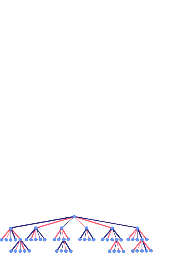
Figure 19: Part of the depth-3 URVG tree $T_{R,3}$.

We now count the vertices on each level $k$ of $T_{R,s}$. For $1\leq k\leq s-1$, let $a_{k}$ be the number of vertices at level $k$ with five children, i.e., those with spine edges to their parents; let $b_{k}$ be the number of vertices at level $k$ with four children, i.e. those with leg edges to their parents; and let $c_{k}=a_{k}+b_{k}$ be the total number of vertices on level $k$.

Note that each vertex $v$ at level $k$ with five children has three children who themselves have five children; the other two children each have four children. If $v$ has four children, then two of them have five children and two of them have four children. We therefore have the following recurrence equations:

$${a_{k}=3a_{k-1}+2b_{k-1},b_{k}=2a_{k-1}+2b_{k-1},a_{1}=4,b_{1}=2.}$$ (1)

Using the fact that $c_{k}=a_{k}+b_{k}$, we can eliminate the $b_{k}$ term to get a system involving $a_{k}$ and $c_{k}$:

$${a_{k}=a_{k-1}+2c_{k-1},c_{k}=a_{k-1}+4c_{k-1},a_{1}=4,c_{1}=6.}$$ (2)

Now let $T$ be any depth-$s$ URV tree, with a decomposition into two UBV forests (one red and one blue) as guaranteed by Theorem 4.5. We say $T$ is a downward tree if every leg extends strictly downward from its point of attachment to its spine. If $T$ is a downward tree, then $T$ is a subtree of $T_{R,s}$, and in fact can be mapped onto $T_{R,s}$ preserving the UBV decomposition. This can be seen easily by induction on $s$. Thus for every downward tree, the bound holds.

Now suppose $T$ has an up-leg, that is, a leg that does not extend strictly downward from its spine. We observe the following consequences of $T$ being a rooted tree:

• Each caterpillar in the decomposition may have at most one such leg.

• This leg must be attached to the highest vertex of the spine.

• This leg must extend strictly upward to its highest vertex and then strictly downward from there.

Consider each vertex $x$ of $T$ in breadth first order. If an up-leg intersects its spine at vertex $x$, we perform the following surgery on $T$. We convert the portion of the spine that is to the left of $x$ to a leg, and convert the up-leg into a spine, extending its terminus downward if necessary until it reaches at least the same depth as the old left side of the spine. We then remove the edge connecting each leg to the old spine, and add an edge connecting the leg to the vertex of the new portion of the spine at precisely the same depth as the one it was attached to on the old spine. All other edges of $T$ remain unchanged. See Figures 20 and 21.

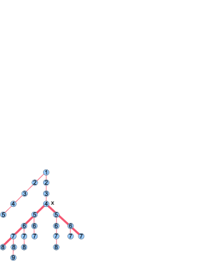
Figure 20: A tree with an up-leg adjacent to vertex $x$. The number on each vertex corresponds to its depth in the tree.

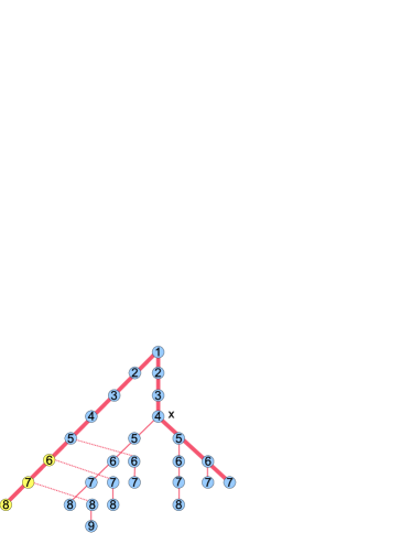
Figure 21: The modified tree, removing the up-leg from Fig. 20. The new edges are represented by dashed lines.

The result is a downward URV tree with at least as many vertices at each depth as the original tree, and hence no more than $c_{k}$ vertices at level $k$.

∎

Standard linear recursion techniques can be used to compute $c_{k}$, either as the coefficient of $x^{k}$ in the generating function $V(x)=\sum_{k=0}^{\infty}{c_{k}x^{k}}$ $=\frac{2(3-x)}{2x^{2}-5x+1}+1$, or in the following closed form:

$$c_{k}= \frac{1}{17}2^{-1-2k}((17-7\sqrt{17})(10-2\sqrt{17})^{k}+$$ (3)

$$2^{1+k}\sqrt{17}(5+\sqrt{17})^{k}+(2(5+\sqrt{17}))^{k}(17+5\sqrt{17})).$$

6.3 Corollary.

If $T$ is a rooted depth-$s$ URV tree, then the maximum number of edges in $T$ is

$$-2+ \left(1-\frac{3}{\sqrt{17}}\right)\left(\frac{1}{2}\left(5-\sqrt{17}\right)\right)^{s}+$$ (4)

$$\left(1+\frac{3}{\sqrt{17}}\right)\left(\frac{1}{2}\left(5+\sqrt{17}\right)\right)^{s}$$

Proof.

This is the sum of Equation (3) as $k$ ranges from 1 to $s$. ∎

Edge bounds for general URVGs

6.4 Theorem.

For $n\geq 1$, let $G$ be a URVG with $n$ vertices. Then $|E(G)|\leq 6n-4\lceil\sqrt{n}\rceil+1$.

Proof.

For $n=1,\ldots,10$ this bound follows immediately from the edge sets of complete graphs. Let $L$ be a URV layout of $G$. Surround the layout $L$ with four rectangles (that are not unit squares) labeled $N,S,E$, and $W$, as shown in Fig. 22. Call the induced rectangle visibility graph $G_{+}$. Partition the edges of $G_{+}$ into the two sets $E=E(G)$ and $E^{\prime}=E(G_{+})-E$. Hence $E^{\prime}$ comprises the edges of $G_{+}$ that have either one or two endpoints in the set $\{N,S,E,W\}$. By a result of ([9], Theorem 1), any rectangle visibility graph with $p\geq 5$ vertices has at most $6p-20$ edges. Therefore,

$$|E|+|E^{\prime}|=|E(G_{+})|\leq 6(n+4)-20=6n+4$$

Now note that the number of edges of $E^{\prime}$ with exactly one end point in $\{N,S,E,W\}$ is at least as large as the number of squares on the perimeter of a rectangle containing all $n$ squares of G. This is at least $\lceil 4\sqrt{n}\rceil$, which is greater than or equal to $4\lceil\sqrt{n}\rceil-3$. There are 6 edges with both endpoints in $\{N,S,E,W\}$, so

$$|E^{\prime}|\geq(4\lceil\sqrt{n}\rceil-3)+6=4\lceil\sqrt{n}\rceil+3.$$

Therefore,

$$|E|\leq 6n+4-|E^{\prime}|\leq 6n+4-(4\lceil\sqrt{n}\rceil+3)\leq 6n-4\lceil\sqrt{n}\rceil+1.$$

∎

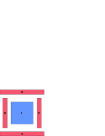
Figure 22: A URV layout plus 4 surrounding rectangles.

Note that, for $5\leq n\leq 25,6n-4\lceil\sqrt{n}\rceil+1\geq 6n-20$, the upper bound established in [9] for any RVG. Hence Theorem 6.4 says something stronger than that result only for $n\geq 26$.

If $B_{n}$ denotes the maximum number of edges among all URVGs with $n$ vertices, then Theorem 6.4 says that $B_{n}\leq 6n-4\lceil\sqrt{n}\rceil+1$. The next theorem uses examples of URVGs with $n\geq 64$ vertices and at least $6n-12\bigl{\lfloor}\sqrt{n}\bigl{\rfloor}+6$ edges to establish that $B_{n}=6n-\Theta(\sqrt{n})$.

6.5 Theorem.

There is a URVG on $n$ vertices with at least $6n-12\bigl{\lfloor}\sqrt{n}\bigl{\rfloor}+6$ edges for each $n\geq 64$.

Proof.

First consider the case when $n=k^{2}$ is a perfect square. Fig. 23, adapted from a figure in [9], shows a layout of a URVG with 64 vertices. The numbers on the squares indicate the degrees of the corresponding vertices, and this example can be extended to give an analogous URVG with $k^{2}$ vertices for $k\geq 8$. For $k\geq 8$, the resulting URVG on $n=k^{2}$ vertices has four vertices of degree 4, four of degree 6, $4(k-3)$ of degree 7, four of degree 10, $4(k-4)$ of degree 11, and the rest of degree 12. Hence the degree sum of this graph is $16+24+28(k-3)+40+44(k-4)+12(k^{2}-8k+16)=12(k-1)^{2}$, and therefore the graph has $6(k-1)^{2}=6n-12\sqrt{n}+6$ edges. Call this graph $G_{n}$.

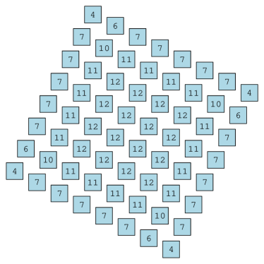
Figure 23: A URV layout with $6n-12\sqrt{n}+6$ edges.

Now suppose $k\geq 8$. We show how to add additional unit squares to an initial layout with $n=k^{2}$ squares to give examples satisfying the condition for $n=k^{2}+1,k^{2}+2,\ldots,k^{2}+2k=(k+1)^{2}-1$. The numbered squares in Fig. 24 are being added to a layout with $n=64=8^{2}$, but the method works for any $n=k^{2}$ with $k\geq 8$. We begin by adding the northeasternmost square labeled 1, which adds one vertex and six new edges to the corresponding graph. We then add, in sequence, the squares labeled $2,3,4,\ldots,k-4$, completing a new row of $k-4$ squares along the upper side of the original layout. Each vertex, when added, increases the edge count by 6. We repeat this process on each of the other three sides of the original layout, adding a total of $4(k-4)$ squares, which is at least $2k$ squares, since $k\geq 8$.

The function $f(n)=6n-12\bigl{\lfloor}\sqrt{n}\bigl{\rfloor}+6$ increases less quickly than the linear function $6n+6$, hence each unit increase of $n$ results in an increase of at most 6 for $f(n)$. Therefore, for $k\geq 8,n=k^{2}$ and $i=0,\ldots,2k-1$, we have by induction that

$$f(n+i+1)\leq f(n+i)+6\leq|E(G_{n+i})|+6\leq|E(G_{n+i+1})|$$

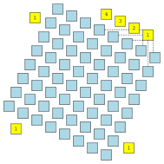
Figure 24: Adding squares to a layout with $k^{2}$ squares.

This establishes the claim of the theorem. ∎

Edge bounds for bipartite URVGs

In ([4], Corollary 10) it is shown that if a bipartite graph $G$ with $n\geq 4$ vertices is a subgraph of an RVG, then $G$ has at most $4n-12$ edges. We use that result to bound the number of edges in a bipartite URVG.

6.6 Theorem.

For $n\geq 7$, let $G$ be a bipartite URVG with $n$ vertices. Then $|E(G)|\leq 4n-2\lceil\sqrt{n}\rceil+5$.

Proof.

Let $G$ be a bipartite graph with $n$ vertices and bipartition $\{A,B\}$, and suppose that $L$ is a URV layout of $G$. As in Fig. 22, surround $L$ with the four rectangles $N,S,E,W$, creating an RVG layout that induces a (non-bipartite) graph on $n+4$ vertices. As in the proof of Theorem 6.4 the number of edges with exactly one endpoint in $\{N,S,E,W\}$ is at least $4\lceil\sqrt{n}\rceil-3$. For each of the four rectangles, $\{N,S,E,W\}$, add it to $A$ if it sees more rectangles from $B$; otherwise add it to $B$. Call the enlarged bipartite sets $A^{\prime}$ and $B^{\prime}$.

Define $G^{\prime}$ to be the bipartite graph induced by the edges with one endpoint in $A^{\prime}$ and the other in $B^{\prime}$. All the edges of $G$ are edges of $G^{\prime}$ and there are at least $2\lceil\sqrt{n}\rceil-1$ bipartite edges with exactly one endpoint in $\{N,S,E,W\}$. By a result of ([4], Corollary 10), the graph $G^{\prime}$ has at most $4(n+4)-12=4n+4$ edges.

If we let $E^{\prime}=E(G^{\prime})\setminus E(G)$, then we have that

$$|E(G)|\leq 4n+4-|E^{\prime}|\leq 4n+4-(2\lceil\sqrt{n}\rceil-1)=4n-2\lceil\sqrt{n}\rceil+5$$

∎

Theorem 6.5 constructed examples of URVGs with $6n-\Theta(\sqrt{n})$ edges. A construction similar to the one in the proof of  that theorem gives examples, for $n\geq 81$, of bipartite graphs with $4n-\Theta(\sqrt{n})$ edges that are URVGs.

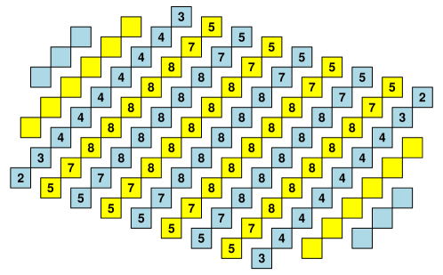
Figure 25: Adding squares to a weak bipartite layout with $k^{2}$ squares.

6.7 Theorem.

For every $n\geq 81$, there is a bipartite graph with $n$ vertices that is a URVG and has at least $4n-8\bigl{\lceil}\sqrt{n}\bigl{\rceil}+4$ edges.

Proof.

As in the proof of Theorem 6.5, we do an initial construction when $n=k^{2}$, and then we show how to handle the cases $n=k^{2}+1,\ldots,k^{2}+2k=(k+1)^{2}-1$. The construction is illustrated with $k=9$ in Fig. 25. The initial array of $k^{2}$ squares (labeled with vertex degrees) has $4k^{2}-8k+4=4n-8\sqrt{n}+4$ edges. We then add the two rows with $k-3$ unlabeled squares, each of which adds four new edges, and then the two rows with $k-6$ unlabeled squares, adding four more edges each. We thus add a total of $2(k-3)+2(k-6)=4k-18$ which is at least $2k$ if $k\geq 9$, and the result follows by the same argument as in the proof of Theorem 6.5. ∎

7 Open Problems

We conclude with two open problems motivated by the work in this paper.

1. Theorem 4.5 says that a tree is a URVG if and only if it is the union of two subdivided caterpillar forests, each with maximum degree 3. The same statement for general graphs is false, because, for example, there are URVGs with maximum degree greater than 6. However, we are not aware of any example of a graph $G$ that is the union of two subdivided caterpillar forests, each with maximum degree 3, that is not a URVG. Note that Theorem 4.6 implies that any such example could not be constructed using two forests of paths.

2. While Theorem 4.5 gives a complete characterization of URVG trees, it does not provide an efficient algorithm to decide whether an arbitrary tree is a URVG. Equivalently, no efficient algorithm is known for deciding if a tree is a union of two subdivided caterpillar forests, each with maximum degree 3. Peroche ([10], Theorem 4) has shown that deciding linear arboricity 2 is NP-complete. Shermer ([14], Theorems 3.2 and 4.5) has shown that deciding caterpillar arboricity 2 is NP-complete, and also that deciding if a graph is an RVG is NP-complete.

References

- [1] P. Bose, A. Dean, J. Hutchinson, and T. Shermer. On rectangle visibility graphs. In Lecture Notes in Computer Science 1190: Graph Drawing, pages 25–44. Springer-Verlag, London, UK, 1997.
- [2] P. Bose, A. Josefczyk, J. Miller, and J. O’Rourke. is a box visibility graph. Technical Report #034, Smith College, 1994.
- [3] A. M. Dean, E. Gethner, and J. P. Hutchinson. Unit bar-visibility layouts of triangulated polygons: Extended abstract. In Lecture Notes in Computer Science 3383: Graph Drawing, pages 111–121. Springer-Verlag, London, UK, 2005.
- [4] A. M. Dean and J. P. Hutchinson. Rectangle-visibility representations of bipartite graphs. In GD ’94: Proceedings of the DIMACS International Workshop on Graph Drawing, pages 159–166, London, UK, 1995. Springer-Verlag.
- [5] A. M. Dean and N. Veytsel. Unit bar-visibility graphs. Congressus Numerantium, 160:161–175, 2003.
- [6] P. Duchet, Y. Hamidoune, M. Las Vergnas, and H. Meyniel. Representing a planar graph by vertical lines joining different levels. Discrete Mathematics, 46:319–321, 1983.
- [7] P. Erdös and A. Szekeres. A combinatorial problem in geometry. Compositio Mathematica, 2:463–470, 1935.
- [8] S. P. Fekete and H. Meijer. Rectangle and box visibility graphs in 3d. International Journal of Computational Geometry and Applications, 9(1):1–21, 1999.
- [9] J. P. Hutchinson, T. Shermer, and A. Vince. On representations of some thickness-two graphs. Computational Geometry, 13:161–171, 1999.
- [10] B. Peroche. Complexité de l’arboricité lineaire d’un graphe. RAIRO Recherche Opérationnelle, 16(2):125–129, 1982.
- [11] P. Rosenstiehl and R. E. Tarjan. Rectilinear planar layouts and bipolar orientations of planar graphs. Discrete & Computational Geometry, 1(4):343–353, 1986.
- [12] M. Schlag, F. Luccio, P. Maestrini, D. Lee, and C. Wong. A visibility problem in VLSI layout compaction. In F. Preparata, editor, Advances in Computing Research, volume 2, pages 259–282. JAI Press Inc., Greenwich, CT, 1985.
- [13] T. Shermer. On rectangle visibility graphs ii: k-hilly and maximum-degree 4. manuscript, 1996.
- [14] T. Shermer. On rectangle visibility graphs iii: external visibility and complexity. In Proceedings of the 8th Canadian Conference on Computational Geometry, pages 234 –239. Carleton University Press, 1996.
- [15] I. Streinu and S. Whitesides. Rectangle visibility graphs: Characterization, construction, and compaction. In STACS ’03: Proceedings of the 20th Annual Symposium on Theoretical Aspects of Computer Science, pages 26–37, London, UK, 2003. Springer-Verlag.
- [16] R. Tamassia and I. G. Tollis. A unified approach to visibility representations of planar graphs. Discrete & Computational Geometry, 1(4):321–341, 1986.
- [17] S. K. Wismath. Characterizing bar line-of-sight graphs. In SCG ’85: Proceedings of the First Annual Symposium on Computational Geometry, pages 147–152, New York, NY, USA, 1985. ACM Press.