Quantum parallelism as a tool for ensemble spin dynamics calculations

Abstract

Efficient simulations of quantum evolutions of spin-$1/2$ systems are relevant for ensemble quantum computation as well as in typical NMR experiments. We propose an efficient method to calculate the dynamics of an observable provided that the initial excitation is “local”. It resorts a single entangled pure initial state built as a superposition, with random phases, of the pure elements that compose the mixture. This ensures self-averaging of any observable, drastically reducing the calculation time. The procedure is tested for two representative systems: a spin star (cluster with random long range interactions) and a spin ladder.

One of the goals of quantum computers is the simulation of quantum systems. While quantum processing is ideally cast in terms of pure states, experimental realizations are a major challenge A Quantum Information Science and Technology Roadmap (2004) met only for very small systems F. H. L. Koppens et al. (2006). The alternative use of statistical mixtures of pure states, as the spin ensembles in standard NMR experiments Zhang et al. (1992); Pastawski et al. (1995); Z. L. Mádi et al. (1997); Vandersypen and Chuang (2004), led to the development of the ensemble quantum computation (EQC) Cory et al. (1998) that allowed useful algorithm optimizations Long and Xiao (2004); Stadelhofer et al. (2005). Recently, EQC was experimentally implemented in a $12$-qubits system C. Negrevergne et al. (2006) and much larger quantum registers Krojanski and Suter (2006) were prepared to assess its stability against decoherence. Hence, an efficient evaluation of ensemble evolutions is needed. Analytical solutions of ensemble dynamics, either from the integration of the Liouville von-Neumann equation Abragam (1961) or the alternative Keldysh formalism Keldysh (1964); Danielewicz (1984) are limited to special cases (e.g. Doronin et al. (2002); Danieli et al. (2005)). Thus, one has to resort to numerical solutions. One can describe an ensemble of $M$ spins by using the $2^{M}\times 2^{M}$ density matrix, but this quickly reaches a storage limit as $M$ increases. Thus, a typical exact diagonalization method in a desktop computer slightly exceeds a dozen of qubits. Alternatively, the use of wave functions combined with the Trotter-Suzuki decomposition Raedt and Michielsen ; W. Zhang et al. overcomes this limitation because it uses vectors of size $2^{M}$. However, the average over individual evolutions of a large number of components of the ensemble takes a long time. Here, this limitation is overcome by profiting of quantum parallelism Schliemann et al. (2005) to evaluate the ensemble dynamics of any observable evolved from a “local” initial condition. The idea is that when evaluated on single pure states that are a superposition of all the elements of the ensemble, these observables become self-averaging. This reinforces the suggestions that one can avoid ensemble or thermal averages by using a single pure state Popescu et al. (2006); Rigol et al. (2008). Ref. Popescu et al. (2006) considers a subsystem with the reduced density matrix derived from a pure state, where the subsystem is entangled with an environment which has a much bigger size. The resulting reduced density matrix describes the microcanonical ensemble without resorting to the equiprobability postulate of statistical mechanics. Following a similar inspiration, we focus on the non-equilibrium dynamics of any given observable. The key is that the initial non-equilibrium state has a “local” character, i.e. starting from an equilibrium ensemble state, a perturbing excitation acts on a small portion of the system. A number of useful techniques to simulate dynamics of a small system in the presence of a mixed-bath that involve averages over random states Gelman and Kosloff (2003); W. Zhang et al. could be interpreted as particular cases. Specifically, an analytical justification of the numerically observed self-averaging property in some particular systems Gelman and Kosloff (2003) follows from our results.

While our method is general and can be applied to any mixed many-body system, we focus on the time evolution of the observable of greatest interest in NMR experiments, the local polarization Zhang et al. (1992); Pastawski et al. (1995); Z. L. Mádi et al. (1997). We consider two spin configurations that are representative of physical situations of contrasting topology. One is a spin ladder which is a variant of the linear chains which are exactly solvable Fabricius et al. (1998); Danieli et al. (2005) and are known to have strong mesoscopic echoes Pastawski et al. (1995); Z. L. Mádi et al. (1997). The other is a spin star, a cluster with random long range interactions which is a fair representation of many molecular crystals Levstein et al. (1998). Here, mesoscopic interferences becomes less intense J. L. Gruver et al. (1997).

Ensemble vs. pure entangled state.— We take the ensemble of all the many-spin states $\left|\Psi_{i}^{m}\right\rangle=\left|\psi_{m}\right\rangle\otimes\left|\Psi_{i}\right\rangle$ where $m$ spins are in the state $\left|\psi_{m}\right\rangle$ and the $\left|\Psi_{i}\right\rangle$ are a base for the remaining $M-m$ spins. These states have a statistical weight $p_{i}$. The probability to find $m^{\prime}$ spins in the state $\left|\psi_{m^{\prime}}\right\rangle$ at time $t$ when the $m$ spins were in state $\left|\psi_{m}\right\rangle$ at $t=0$ is

$$W_{m^{\prime}m}^{\mathrm{ens}}(t)=\sum_{f=1}^{2^{M-m^{\prime}}}\sum_{i=1}^{2^{M-m}}p_{i}\left|\left\langle\Psi_{f}^{m^{\prime}}\right|e^{-\mathrm{i}\widehat{\mathcal{H}}t/\hbar}\left|\Psi_{i}^{m}\right\rangle\right|^{2}.$$ (1)

Here, $\left|\left\langle\Psi_{f}^{m^{\prime}}\right|e^{-\mathrm{i}\widehat{\mathcal{H}}t/\hbar}\left|\Psi_{i}^{m}\right\rangle\right|^{2}$ is the probability of finding $m^{\prime}$ spins in the state $\left|\psi_{m^{\prime}}\right\rangle$ within the many-spin state $\left|\Psi_{f}^{m^{\prime}}\right\rangle$ at time $t$ provided that, at $t=0,$ the $m$ spins were in the state $\left|\psi_{m}\right\rangle$ within the state $\left|\Psi_{i}^{m}\right\rangle$. The sum runs over all possible initial and final states. An example of this is the local correlation function where $m=m^{\prime}=1,$ $\left|\psi_{m}\right\rangle=\left|\uparrow\right\rangle_{n}$ is the state of the $n$-th spin and $\left|\psi_{m^{\prime}}\right\rangle=\left|\uparrow\right\rangle_{n^{\prime}}$ is the state of spin $n^{\prime}$. The polarization of spin $n^{\prime}$ at time $t$ provided that the spin $n$ was up at time $t=0$ is given by $P_{n^{\prime}n}^{\mathrm{ens}}\left(t\right)=2[W_{11}^{\mathrm{ens}}(t)-1/2]$ Pastawski et al. (1995). The expression (1) involves $D=2^{M-m}$ different dynamics for each of the initial states, see Fig. 1(a).

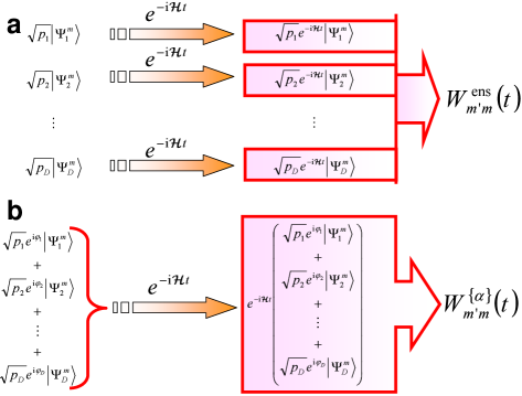
Figure 1: (Color online) Schemes of the quantum evolution of an ensemble (panel (a)) and a pure-state (panel (b)). Each $\left|\Psi_{i}^{m}\right\rangle=\left|\psi_{m}\right\rangle\otimes\left|\Psi_{i}\right\rangle$ contains a complete base, $\left|\Psi_{i}\right\rangle$, of the $M-m$ spins.

This number is directly related to the dimension of the Hilbert space. Thus, the number of computed evolutions increases exponentially with $M$. Our goal is to extract the same information in a shorter time. The parallelism implicit in quantum superpositions Schliemann et al. (2005) suggests that the desired correlation functions are contained in the dynamics of a single pure-state, see Fig. 1(b). The pure-state is built as an arbitrary linear superposition of components of the ensemble, i.e. $\left|\Psi_{\mathrm{pure}}^{\{\alpha\}}\right\rangle=\sum_{i=1}^{D}\alpha_{i}\left|\Psi_{i}^{m}\right\rangle$ where $\alpha_{i}=\sqrt{p_{i}}e^{\mathrm{i}\varphi_{i}}$ with random $\varphi_{i}$. Thus, the correlation function is given by

$$W_{m^{\prime}m}^{\{\alpha\}}(t)={\textstyle\sum\limits_{f=1}^{D^{\prime}}}\left|\left\langle\Psi_{f}^{m^{\prime}}\right|e^{-\mathrm{i}\widehat{\mathcal{H}}t/\hbar}\sum\limits_{i=1}^{D}\alpha_{i}\left|\Psi_{i}^{m}\right\rangle\right|^{2}.$$ (2)

Here $\{\alpha\}$ denotes the set of all the $\alpha_{i}$ involved in the initial pure-state and $D^{\prime}=2^{M-m^{\prime}}$. Note that the substantial difference between Eq. (1) and Eq. (2) is that the sum on $i$ in the former is outside the square modulus while in the latter is inside. Rewriting Eq. (2) as

$$W_{m^{\prime}m}^{\{\alpha\}}(t)={\textstyle\sum\limits_{f=1}^{D^{\prime}}}{\textstyle\sum\limits_{i=1}^{D}}p_{i}\left|\left\langle\Psi_{f}^{m^{\prime}}\right|e^{-\mathrm{i}\widehat{\mathcal{H}}t/\hbar}\left|\Psi_{i}^{m}\right\rangle\right|^{2}$$ (3)

$$+{\textstyle\sum\limits_{f=1}^{D^{\prime}}}{\textstyle\sum\limits_{i\neq i^{\prime}=1}^{D}}\alpha_{i}\alpha_{i^{\prime}}^{\ast}\left\langle\Psi_{i^{\prime}}^{m}\right|e^{\mathrm{i}\widehat{\mathcal{H}}t/\hbar}\left|\Psi_{f}^{m^{\prime}}\right\rangle\left\langle\Psi_{f}^{m^{\prime}}\right|e^{-\mathrm{i}\widehat{\mathcal{H}}t/\hbar}\left|\Psi_{i}^{m}\right\rangle,$$

the second term contains the initial correlations between the components of the initial state. These cross terms make the difference between $W_{m^{\prime}m}^{\mathrm{ens}}(t)$ and $W_{m^{\prime}m}^{\{\alpha\}}(t).$ By performing an extra average over $N_{\alpha}$ realizations of the possible initial states, we obtain

$$\left\langle W_{m^{\prime}m}^{\{\alpha\}}(t)\right\rangle_{N_{\alpha}}=\frac{1}{N_{\alpha}}{\textstyle\sum\limits_{\{\alpha\}}^{N_{\alpha}}}W_{m^{\prime}m}^{\{\alpha\}}(t).$$ (4)

Under this average, each element in the cross term goes to zero, hence $W_{m^{\prime}m}^{\mathrm{ens}}(t)=\lim_{N_{\alpha}\rightarrow\infty}\left\langle W_{m^{\prime}m}^{\{\alpha\}}(t)\right\rangle_{N_{\alpha}}$. Thus, by increasing the number $N_{\alpha}$ of evolutions, expression (4) converges to $W_{m^{\prime}m}^{\mathrm{ens}}(t)$ as described by the central limit theorem.  The variance of $W_{m^{\prime}m}^{\{\alpha\}}(t)$ is $\mathrm{Var}=\lim_{N_{\alpha}\rightarrow\infty}\left\langle W_{m^{\prime}m}^{\{\alpha\}}(t)^{2}\right\rangle_{N_{\alpha}}-\left\langle W_{m^{\prime}m}^{\{\alpha\}}(t)\right\rangle_{N_{\alpha}}^{2}.$ At this stage, the four phases $\varphi_{i}$ summing up in each exponent are correlated. This enables terms where the exponent cancels out. These survive the average and contribute to $\mathrm{Var}=~{}{\textstyle\sum\nolimits_{i\neq i^{\prime}=1}^{D}}p_{i}p_{i^{\prime}}\left|\left\langle\Psi_{i^{\prime}}^{m}\right|e^{\mathrm{i}\widehat{\mathcal{H}}t/\hbar}\hat{P}_{f}e^{-\mathrm{i}\widehat{\mathcal{H}}t/\hbar}\left|\Psi_{i}^{m}\right\rangle\right|^{2}$ where $\hat{P}_{f}={\textstyle\sum\nolimits_{f}^{D^{\prime}}}\left|\Psi_{f}^{m^{\prime}}\right\rangle\left\langle\Psi_{f}^{m^{\prime}}\right|$. In the last expression $\left|\left\langle\Psi_{i^{\prime}}^{m}\right|e^{\mathrm{i}\widehat{\mathcal{H}}t/\hbar}\hat{P}_{f}e^{-\mathrm{i}\widehat{\mathcal{H}}t/\hbar}\left|\Psi_{i}^{m}\right\rangle\right|^{2}=w_{i^{\prime}i}$ is the probability to find the state $\left|\Psi_{i^{\prime}}^{m}\right\rangle$ after the subunitary evolution $e^{\mathrm{i}\widehat{\mathcal{H}}t/\hbar}\hat{P}_{f}e^{-\mathrm{i}\widehat{\mathcal{H}}t/\hbar}$ provided that the initial state was $\left|\Psi_{i}^{m}\right\rangle.$ The projector $\hat{P}_{f}$ involves only part of the Hilbert space states. Hence, ${\textstyle\sum\nolimits_{i^{\prime}}^{D}}w_{i^{\prime}i}\leq 1\$implies $\mathrm{Var}=$ ${\textstyle\sum\nolimits_{\genfrac{}{}{0.0pt}{}{i,i^{\prime}=1}{i\neq i^{\prime}}}^{D}}p_{i}p_{i^{\prime}}~{}w_{i^{\prime}i}\leq$ ${\textstyle\sum\nolimits_{i}^{D}}p_{i}\max\left\{p_{i^{\prime}}\right\}=$ $\max\left\{p_{i^{\prime}}\right\}.$ Thus, by using the Chebyshev’s Inequality the probability that $\left|\left\langle W_{m^{\prime}m}^{\{\alpha\}}(t)\right\rangle_{N_{\alpha}}-W_{m^{\prime}m}^{\mathrm{ens}}(t)\right|\geq\varepsilon$ (i.e. the error exceeds a desired precision $\varepsilon$) is lower than $\mathrm{Var}/\left(N_{\alpha}\varepsilon^{2}\right)\leq$ $\max\left\{p_{i^{\prime}}\right\}/\left(N_{\alpha}\varepsilon^{2}\right).$ For an homogeneous distribution $p_{i}=1/2^{M-m}$ hence $\max\left\{p_{i^{\prime}}\right\}/\left(N_{\alpha}\varepsilon^{2}\right)=$ $2/\left(2^{M-m}N_{\alpha}\varepsilon^{2}\right).$ The locality of the initial condition ensures that $M\gg m,$ thus, as $2^{M-m}\$increases, one gets $W_{m^{\prime}m}^{\{\alpha\}}(t)\approx W_{m^{\prime}m}^{\mathrm{ens}}(t)$ in a single realization, i.e. the cross terms in Eq. (3) self-average to zero even for $N_{\alpha}=1$.

Spin systems with different coupling networks.— To illustrate the use of Eq. (4) we consider typical situations of high-field solid-state NMR. Here, the Hamiltonian is simplified by using a frame that eliminates the Zeeman contribution Abragam (1961). We are left with the spin-spin interaction, $\widehat{\mathcal{H}}={\textstyle\sum\nolimits_{i<j}^{M}}\left[a_{ij}\hat{I}_{i}^{z}\hat{I}_{j}^{z}+\tfrac{1}{2}b_{ij}\left(\hat{I}_{i}^{+}\hat{I}_{j}^{-}+\hat{I}_{i}^{-}\hat{I}_{j}^{+}\right)\right],$where $b_{ij}/a_{ij}=0$ represents an Ising-like coupling, $a_{ij}/b_{ij}=0$ an $XY$ Hamiltonian, $a_{ij}/b_{ij}=1$ the isotropic one, and $a_{ij}/b_{ij}=-2$ a dipolar (secular) Hamiltonian truncated with respect to a Zeeman field along the $z$ axis. The ensemble relevant for NMR experiments is in the infinite temperature limit Abragam (1961); Vandersypen and Chuang (2004), i.e., $p_{i}=1/2^{M-1}\$where $\left|\Psi_{i}\right\rangle\$are simple tensor product states in the Zeeman basis. The initial conditions are states with a local excitation at site $n$ over a background level which is determined by the zero magnetization of the other $M-1$ spins Zhang et al. (1992); Pastawski et al. (1995); Z. L. Mádi et al. (1997).

We calculate the local polarization of site $n^{\prime}$ at time $t$ provided that it was polarized ($n=n^{\prime}$) at time $t=0$ in two different spin systems which have well differentiated kinds of dynamics:

a) A ladder of spins interacting through an XY Hamiltonian, as shown in Fig. 2(a). There, $a_{ij}=0,$ $b_{i,i+1}=b_{i+M/2,i+M/2+1}=b_{x}$ and $b_{i,i+M/2}=b_{y}$. Here, the exact dynamics presents long lived recurrences (mesoscopic echoes) shown by the black line in Fig. 3(a), due to the high symmetry in the coupling topology Pastawski et al. (1995); Z. L. Mádi et al. (1997). The method also reproduces the exact solutions in isolated spin chains with both, pure XY or XY plus Ising interactions Fabricius et al. (1998). Moreover, the results confirm that inclusion of Ising terms or interchain couplings leads to decoherence degrading the mesoscopic echoes Z. L. Mádi et al. (1997).

b) A star system, see Fig. 2(b), in which all the spins interact with each other through a dipolar coupling $a_{ij}/b_{ij}=-2$. The coupling intensities are given by a Gaussian random distribution with zero mean and variance $\sigma^{2}$. In this case, the local polarization decays with a rate proportional to the square root of the local second moment $\sigma_{0}^{2}=\frac{9}{4}\left(M-1\right)\sigma^{2}$ Abragam (1961) of the Hamiltonian and recurrences are negligible J. L. Gruver et al. (1997). The black line (exact solution) of Fig. 3(b) shows the local polarization of this system.

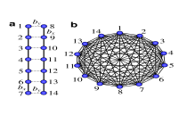
Figure 2: (Color online) Panel (a) shows the coupling network of a spin ladder. Panel (b) contains the coupling network of a spin star in which all the spins interact with each other.

Testing the quantum parallelism.— In order to compare Eq. (4) to the ensemble average of Eq. (1), as well as its dependence on the choice of the phases $\varphi_{i}$, we calculate the evolution for two types of initial states. Firstly, a pure entangled state is constructed by choosing $\varphi_{i}$ randomly. Thus, assuming $n=1,$ $\left|\Psi_{\mathrm{pure}}^{\{\alpha\}}\right\rangle$ becomes $\left|\Psi_{\mathrm{ent}}^{\{\alpha\}}\right\rangle=$ ${\textstyle\sum_{i=1}^{2^{M-1}}}\tfrac{1}{\sqrt{2^{M-1}}}e^{-\mathrm{i}\varphi_{i}}\left|\uparrow\right\rangle_{1}\otimes\left|\Psi_{i}\right\rangle.$ The correlation function, Eq. (4), calculated with this state is $\left\langle W_{11}^{\mathrm{ent}}(t)\right\rangle_{N_{\alpha}}$ giving the polarization $\left\langle P_{11}^{\mathrm{ent}}(t)\right\rangle_{N_{\alpha}}=$ $2\left(\left\langle W_{11}^{\mathrm{ent}}(t)\right\rangle_{N_{\alpha}}-1/2\right)$. The second case is a product (not entangled) state. It is built with the $n$-th spin up and all the others in a linear combination of spins up and down, with equal probability and arbitrary phase. Assuming $n=1$, we have $\left|\Psi_{\mathrm{prod}}^{\{\alpha\}}\right\rangle=$ $\left|\uparrow\right\rangle_{1}{\textstyle\bigotimes}\prod\limits_{l=2}^{M}\left|\rightarrow\right\rangle_{l},$ where $\left|\rightarrow\right\rangle_{l}=$ $\tfrac{1}{\sqrt{2}}\left(\left|\downarrow\right\rangle_{l}+\left|\uparrow\right\rangle_{l}e^{-\mathrm{i}\phi_{l}}\right)$ with $\phi_{l}$ random variables. Note that this state can be rewritten in the form of $\left|\Psi_{\mathrm{pure}}^{\{\alpha\}}\right\rangle$ where the resulting phases $\varphi_{i}$ are correlated. Here, the correlation function (4) is $\left\langle W_{11}^{\mathrm{prod}}(t)\right\rangle_{N_{\alpha}}$ and the polarization is $\left\langle P_{11}^{\mathrm{prod}}(t)\right\rangle_{N_{\alpha}}=$ $2\left\langle W_{11}^{\mathrm{prod}}(t)\right\rangle_{N_{\alpha}}-1.$

The local polarization, $P_{11}^{\mathrm{ens}}(t)=2\left(W_{11}^{\mathrm{ens}}(t)-1/2\right),$ obtained with Eq. (1), for the $14$-spin ladder system is shown in Fig. 3(a) with a black line.

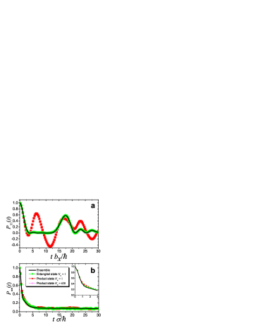
Figure 3: (Color online) Local spin dynamics in a $14$-spin system. The ensemble dynamics (solid line) is compared with that of entangled and product pure states. The square (red) and circle (green) scatter points correspond to $\left\langle P_{11}^{\mathrm{prod}}(t)\right\rangle_{N_{\alpha}}$ and $\left\langle P_{11}^{\mathrm{ent}}(t)\right\rangle_{N_{\alpha}}$ for $N_{\alpha}=1$ respectively. (a) The extreme of a spin ladder with $b_{y}/b_{x}=1/10.$ The triangle scatter points (light magenta) correspond to $\left\langle P_{11}^{\mathrm{prod}}(t)\right\rangle_{N_{\alpha}}$ with $N_{\alpha}=630,$ the lower value yielding the ensemble dynamics. A strong mesoscopic echo is evident. (b) A site in a spin star with random dipolar interactions. No mesoscopic echo is evident.

Square (red) and circle (green) scatter lines correspond to the temporal evolution of $\left\langle P_{11}^{\mathrm{prod}}(t)\right\rangle_{N_{\alpha}}$ and $\left\langle P_{11}^{\mathrm{ent}}(t)\right\rangle_{N_{\alpha}}\$respectively, with $N_{\alpha}=1$. The agreement between $P_{11}^{\mathrm{ens}}(t)$ and $\left\langle P_{11}^{\mathrm{ent}}(t)\right\rangle_{1}$ is excellent, while $\left\langle P_{11}^{\mathrm{prod}}(t)\right\rangle_{1}$ has a dynamics quite different from that of the ensemble. The difference between the dynamics of the two initial pure states is due to the different number of independent random phases of each state. In the random entangled state, there are $2^{M-1}$ independent phases that make the cancellation of the second term in the rhs of Eq. (3) possible. However, the number of independent phases for the product state is $M-1$. This implies that there are multiple correlations between the phases in the cross terms inhibiting their self cancellation. The triangle (light magenta) scatter line in Fig. 3(a) shows the dynamics of $\left\langle P_{11}^{\mathrm{prod}}(t)\right\rangle_{N_{\alpha}}.$ It becomes indistinguishable from the exact dynamics provided that $N_{\alpha}\gtrsim 630$. The relation between $N_{\alpha}^{\mathrm{prod}}=630$ and $N_{\alpha}^{\mathrm{ent}}=1$ is determined by the number of independent phases associated with the dimension of the sampled portion of the Hilbert space Popescu et al. (2006), i.e. $8192=N_{\alpha}^{\mathrm{ent}}2^{M-1}\simeq N_{\alpha}^{\mathrm{prod}}(M-1)=8190.$

Fig. 3(b) shows the local polarization for the spin star system. The complexity of this system washes out any possible recurrence for long times leading to a form of spin “diffusion”. For $N_{\alpha}=1$ both $\left\langle P_{11}^{\mathrm{prod}}(t)\right\rangle_{1}$ and $\left\langle P_{11}^{\mathrm{ent}}(t)\right\rangle_{1}$ are almost indistinguishable from the ensemble dynamics. This contrasts with the spin ladder where one would need $\left\langle P_{11}^{\mathrm{prod}}(t)\right\rangle_{630}$ to get a fair description. Notably, $\left\langle P_{11}^{\mathrm{ent}}(t)\right\rangle_{1}$ is an excelent approximant of the ensemble for both cases. This is because, in the star system the cross terms $\left\langle\Psi_{f}^{1}\right|e^{-\mathrm{i}\widehat{\mathcal{H}}t/\hbar}\left|\Psi_{i}^{1}\right\rangle\left\langle\Psi_{i^{\prime}}^{1}\right|e^{\mathrm{i}\widehat{\mathcal{H}}t/\hbar}\left|\Psi_{f}^{1}\right\rangle$ of Eq. (3) decay to a value of the order of $1/2^{M}$ within a time scale determined by the Hamiltonian second moment $\sigma_{\mathcal{H}}^{2}=\frac{M}{2}\sigma_{0}^{2}.$ Thus, even the few $M$ independent phases are enough to cancel the cross terms. In contrast, in the ladder system, the terms $\left\langle\Psi_{f}^{1}\right|e^{-\mathrm{i}\widehat{\mathcal{H}}t/\hbar}\left|\Psi_{i}^{1}\right\rangle\left\langle\Psi_{i^{\prime}}^{1}\right|e^{\mathrm{i}\widehat{\mathcal{H}}t/\hbar}\left|\Psi_{f}^{1}\right\rangle$ present strong correlations and thus, the role of the phases becomes more relevant.

In summary, we developed a method to overcome the limitations of the numerical calculations of an ensemble spin dynamics for large number of spins. Instead of evolving every one of the $2^{M-m}$ initial states, when $2^{M}\gg 2^{m},$ we evolve a single random entangled state. The procedure exploits the quantum parallelism implicit in quantum superpositions Schliemann et al. (2005) to reproduce the ensemble dynamics of any observable. This result supports a novel view of the foundation of equilibrium statistical mechanics Popescu et al. (2006); Rigol et al. (2008). Moreover, even the non-equilibrium statistical theory of the density matrix describing an ensemble in the thermodynamic limit could now be based on single states. Here, we observe that even for systems as small as $14$ spins, the equivalence between a randomly correlated pure-state and an ensemble state holds. This is a consequence of the exponential increase of the dimension of the Hilbert space with the system size. The power of the method is enhanced when combined with the Trotter-Suzuki decomposition. We showed that the contribution of the extra correlations of the initial pure-state to the dynamics becomes negligible by increasing $2^{M-m}$, the ratio between the size of the system Hilbert space and that of the subsystem where the non-equilibrium initial condition is supported. The method developed here allows for very efficient dynamical calculations of common experimental situations where large ensembles are involved. Conversely, it prescribes possible pure input states for a quantum simulator to yield ensemble evolutions.

References

A Quantum Information Science and Technology
Roadmap (2004)
A Quantum Information Science and Technology
Roadmap, http://qist.lanl.gov/ (2004).
F. H. L. Koppens et al. (2006)
F. H. L. Koppens et al.,
Nature (London) 442,
766 (2006); Y. Wu et al., Phys. Rev. Lett.
96, 087402 (2006); M. Grajcar et al., ibid.96, 047006 (2006); M. Riebe et al., ibid.97, 220407 (2006).
Zhang et al. (1992)
S. Zhang,
B. Meier, and
R. Ernst,
Phys. Rev Lett. 69,
2149 (1992).
Pastawski et al. (1995)
H. M. Pastawski,
P. R. Levstein,
and G. Usaj,
Phys. Rev. Lett. 75,
4310 (1995).
Z. L. Mádi et al. (1997)
Z. L. Mádi et al.,
Chem. Phys. Lett. 268,
300 (1997).
Vandersypen and Chuang (2004)
L. M. K. Vandersypen
and I. L.
Chuang, Rev. Mod. Phys.
76, 1037 (2004).
Cory et al. (1998)
D. G. Cory,
A. F. Fahmy, and
T. F. Havel,
Proc. Natl. Acad. Sci. USA 94,
1634 (1997); N. A. Gershenfeld and I. L. Chuang, Science
275, 350 (1997); E. Knill and R. Laflamme, Phys. Rev. Lett.
81, 5672 (1998).
Long and Xiao (2004)
G. L. Long and
L. Xiao,
Phys. Rev A 69,
052303 (2004).
Stadelhofer et al. (2005)
R. Stadelhofer,
D. Suter, and
W. Banzhaf,
Phys. Rev. A 71,
032345 (2005).
C. Negrevergne et
al. (2006)
C. Negrevergne et al.,
Phys. Rev. Lett. 96,
170501 (2006).
Krojanski and Suter (2006)
H. G. Krojanski
and D. Suter,
Phys. Rev. Lett. 93,
090501 (2004); ibid.97, 150503
(2006).
Abragam (1961)
A. Abragam,
Principles of Nuclear Magnetism
(Oxford University Press, London, 1961).
Keldysh (1964)
L. V. Keldysh,
ZhETF 47, 1515.
[Sov. Phys. (1964).
Danielewicz (1984)
P. Danielewicz,
Ann. Phys. 152,
239 (1984).
Doronin et al. (2002)
S. I. Doronin,
E. B. Fel’dman,
and S. Lacelle,
J. Chem. Phys. 117,
9646 (2002).
Danieli et al. (2005)
E. P. Danieli,
H. M. Pastawski,
and G. A.
Álvarez, Chem. Phys. Lett.
402, 88 (2005).
(17)
H. D. Raedt and
K. Michielsen,
quant-ph/0406210.
(18)
W. Zhang et al.,
J. Phys.: Condens. Matter 19,
083202 (2007), and references therein.
Schliemann et al. (2005)
J. Schliemann,
A. V. Khaetskii,
and D. Loss,
Phys. Rev. B 66,
245303 (2002); B. Paredes, F. Verstraete, and J. I. Cirac,
Phys. Rev. Lett. 95, 140501 (2005).
Popescu et al. (2006)
S. Popescu,
A. J. Short, and
A. Winter,
Nat. Phys. 2,
754 (2006).
Rigol et al. (2008)
M. Rigol,
V. Dunjko, and
M. Olshanii,
Nature 452,
854 (2008).
Gelman and Kosloff (2003)
D. Gelman and
R. Kosloff,
Chem. Phys. Lett. 381,
129 (2003).
Fabricius et al. (1998)
K. Fabricius,
U. Löw, and
J. Stolze,
Phys. Rev. B 55,
5833 (1997); K. Fabricius and B. M. McCoy, ibid.57, 8340 (1998).
Levstein et al. (1998)
P. R. Levstein,
G. Usaj, and
H. M. Pastawski,
J. Chem. Phys. 108,
2718 (1998).
J. L. Gruver et al. (1997)
J. L. Gruver et al.,
Phys. Rev. E 55,
6370 (1997).