Measurement of the $K_{L}$ $\rightarrow$ $\pi\mu\nu$ form factor parameters with the KLOE detector

Abstract:

Using 328 pb^-1of data collected at DAΦNE corresponding to $\sim$1.8 million $K_{L}\rightarrow\pi\mu\nu$ decays, we have measured the $K_{\mu 3}$ form factor parameters. The structure of the $K-\pi$ vector-current provides information about the dynamics of the strong interaction; its knowledge is necessary for evaluation of the phase-space integral required for measuring the CKM matrix element $V_{us}$ and for testing lepton universality in kaon decays. Using a new parametrization for the vector and scalar form factors, we find $\lambda_{+}$=$(25.7\pm 0.6)\times 10^{-3}$ and $\lambda_{0}$=$(14.0\pm 2.1)\times 10^{-3}$. Our result for $\lambda_{0}$, together with recent lattice calculations of $f_{\pi}$, $f_{K}$ and $f(0)$, satisfies the Callan-Treiman relation.

1 Introduction

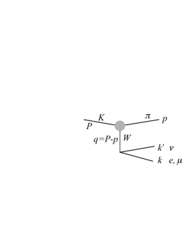
Figure 1: Amplitude for $K_{L}\rightarrow\pi^{\pm}\ell^{\mp}\nu$. The gray circle indicates the $K\pi W$ vertex structure.

Semileptonic kaon decays, $K_{L}\rightarrow\pi^{\pm}\ell^{\mp}\nu$,(Fig. 1) offer possibly the cleanest way to obtain an accurate value of the Cabibbo angle, or better, $V_{us}$. Since $K\rightarrow\pi$ is a $0^{-}\rightarrow 0^{-}$ transition, only the vector part of the hadronic weak current has a non-vanishing contribution. Vector transitions are protected by the Ademollo-Gatto theorem against SU(3) breaking corrections to lowest order in $m_{s}$ (or $m_{s}-m_{u,d}$). At present, the largest uncertainty in calculating $V_{us}$ from the decay rate is due to the difficulties in computing the matrix element $\langle\pi|J^{\rm had}_{\alpha}|K\rangle$. In the notation of Fig. 1, Lorentz invariance requires that this matrix element have the form

$$\langle\pi|J^{\rm had}_{\alpha}|K\rangle=(P+p)_{\alpha}\>f_{+}(t)+(P-p)_{\alpha}\>f_{-}(t)$$ (1)

where $t=(P-p)^{2}=(k+k^{\prime})^{2}=M^{2}+m^{2}-2ME_{\pi}$ is the only $L$-invariant variable. The form factors (FF) $f_{+}(t)$ and $f_{-}(t)$ account for the non-pointlike structure of the hadrons; the values of the FFs at $t=0$ differ from unity because of $SU(3)$ corrections, i.e., because pions and kaons have different structure. The term containing $f_{-}$ is negligible for $K_{e3}$ decays, because the coefficient $P-p=k+k^{\prime}$, when acting on the leptonic current, gives the lepton mass. The FF $f_{-}$ must be retained for $K_{\mu 3}$ decays. It is customary to introduce a scalar FF $f_{0}(t)$, such that Eq. (1) becomes

$$\langle\pi|J^{\rm had}_{\alpha}|K\rangle=f(0)\left[(P+p)_{\alpha}\>\tilde{f}_{+}(t)+(P-p)_{\alpha}\>\left(\tilde{f}_{0}(t)\,{\Delta_{K\pi}\over t}-\tilde{f}_{+}(t)\,{\Delta_{K\pi}\over t}\right)\right],$$

with $\Delta_{K\pi}=M^{2}-m^{2}$. Since the FFs $f_{+}$ and $f_{0}$ must have the same value at $t=0$, the term $f(0)$ has been factored out. The functions $\tilde{f}_{+}(t)$ and $\tilde{f}_{0}(t)$ are therefore both unity at $t=0$. If the FFs are expanded in powers of $t$ up to $t^{2}$ as

$$\tilde{f}_{+,0}(t)=1+\lambda^{\prime}_{+,0}~{}\frac{t}{m^{2}}+\frac{1}{2}\;\lambda^{\prime\prime}_{+,0}\,\left(\frac{t}{m^{2}}\right)^{2}$$ (2)

four parameters ($\lambda^{\prime}_{+}$, $\lambda^{\prime\prime}_{+}$, $\lambda^{\prime}_{0}$, and $\lambda^{\prime\prime}_{0}$) need to be determined from the decay spectrum in order to be able to compute the phase space integral that appears in the formula for the partial decay width. However, this parametrization of the FFs is problematic, because the values for the $\lambda$s obtained from fits to the experimental decay spectrum are strongly correlated, as discussed in the Appendix and in Ref. [5]. In particular, the correlation between $\lambda^{\prime}_{0}$ and $\lambda^{\prime\prime}_{0}$ is $-99.96\%$; that between $\lambda^{\prime}_{+}$ and $\lambda^{\prime\prime}_{+}$ is $-97.6\%$. It is therefore impossible to obtain meaningful results using this parameterization.

Form factors can also by described by a pole form:

$$\mbox{$\tilde{f}_{+}(t)$}_{+,0}={M_{V,S}^{2}\over M_{V,S}^{2}-t},$$ (3)

which expands to $1+t/M_{V,S}^{2}+(t/M_{V,S}^{2})^{2}$, neglecting powers of $t$ greater than 2. It is not clear however what vector and scalar states should be used.

Recent $K_{e3}$ measurements[2, 3, 4] show that the vector FF is dominated by the closest vector $(q\bar{q})$ state with one strange and one light quark (or $K\pi$ resonance, in an older language). The pole-fit results are also consistent with predictions from a dispersive approach [6, 7, 8]. We will therefore use a parametrization for the vector FF based on a dispersion relation twice subtracted at $t=0$ [7]:

$$\mbox{$\tilde{f}_{+}(t)$}=\exp\left[\frac{t}{m_{\pi}^{2}}\left(\Lambda_{+}+H(t)\right)\right],$$ (4)

where $H(t)$ is obtained using $K-\pi$ scattering data, and $\tilde{f}_{+}(0)=1$, $\tilde{f}^{\prime}_{+}(0)=\Lambda_{+}/m_{\pi}^{2}$ . A good approximation to Eq. (4) is

$$\mbox{$\tilde{f}_{+}(t)$}=1+\lambda_{+}{t\over m^{2}}+{\lambda_{+}^{2}+0.000584\over 2}\left(t\over m^{2}\right)^{2}+{\lambda_{+}^{3}+3\times 0.000584\,\lambda_{+}+0.0000299\over 6}\left(t\over m^{2}\right)^{3}.$$

The errors on the constants 0.000584 and 0.0000299 in Eq. (1) are 0.00009 and 0.000002, respectively. The pion spectrum in $K_{\mu 3}$ decay has also been measured recently [2, 9, 10]. As discussed in the Appendix, there is no sensitivity to $\lambda^{\prime\prime}_{0}$. All authors have fitted their data using a linear scalar FF:

$$\mbox{$\tilde{f}_{0}(t)$}=1+\lambda_{0}{t\over m^{2}}.$$ (5)

Because of the strong correlation between $\lambda_{0}^{\prime}$ and $\lambda_{0}^{\prime\prime}$, use of the linear rather than the quadratic parameterization gives a value for $\lambda_{0}$ that is greater than $\lambda_{0}^{\prime}$ by an amount equal to about 3.5 times the value of $\lambda_{0}^{\prime\prime}$. To clarify this situation, it is necessary to obtain a form for $\tilde{f}_{0}(t)$ with $t$ and $t^{2}$ terms but with only one parameter.

The Callan-Treiman relation[11] fixes the value of scalar FF at $t=\Delta_{K\pi}$ (the so-called Callan-Treiman point) to the ratio of the pseudoscalar decay constants $f_{K}/f_{\pi}$. This relation is slightly modified by SU(2)-breaking corrections[12]:

$$\tilde{f}_{0}(\Delta_{K\pi})=\frac{f_{K}}{f_{\pi}}\>{1\over f(0)}+\Delta_{CT},\quad\Delta_{CT}\simeq-3.4\times 10^{-3}$$ (6)

A recent parametrization for the scalar FF [6] allows the constraint given by the Callan-Treiman relation to be exploited. It is a twice-subtracted representation of the FF at $t=\Delta_{K\pi}$ and $t=0$:

$$\tilde{f}_{0}(t)=\exp\left(\frac{t}{\Delta_{K\pi}}\log(C-G(t))\right)$$ (7)

such that $C=\tilde{f}_{0}(\Delta_{K\pi})$ and $\tilde{f}_{0}(t)=1$. $G(t)$ is derived from $K\pi$ scattering data. As suggested in Ref. [6], a good approximation to Eq. (7) is

 

$${\mbox{$\tilde{f}_{0}(t)$}=1+\lambda_{0}{t\over m^{2}}+{\lambda_{0}^{2}+0.000416\over 2}\left({t\over m^{2}}\right)^{2}+{\lambda_{0}^{3}+3\times 0.000416\,\lambda_{0}+0.0000272\over 6}\left({t\over m^{2}}\right)^{3}.}$$

  (8)

with $\log C=\lambda_{0}\Delta_{K\pi}/m^{2}_{\pi}+0.0398\pm 0.0041$. Eq. (8) is quite similar to the result in Ref. [13]. The errors on the constants 0.000416 and 0.0000272 in Eq. (8) are 0.00005 and 0.000001, respectively.

At KLOE, the pion energy and therefore $t$ can be measured, since the $K_{L}$ momentum is known at a $\phi$ factory. However, $\pi$-$\mu$ separation is very difficult at low energy. Attempts to distinguish pions and muons result in a loss of events of more than 50% and introduce severe systematic uncertainties. We therefore use the neutrino spectrum, which can be obtained without $\pi$-$\mu$ identification.

2 The KLOE detector

The KLOE detector consists of a large cylindrical drift chamber, surrounded by a lead scintillating-fiber electromagnetic calorimeter. A superconducting coil around the calorimeter provides a 0.52 T field. The drift chamber [14] is 4 m in diameter and 3.3 m long. The momentum resolution is $\sigma_{p_{\perp}}/p_{\perp}\approx 0.4\%$. Two-track vertices are reconstructed with a spatial resolution of $\sim$3 mm.

The calorimeter [15] is divided into a barrel and two endcaps. It covers 98% of the solid angle. Hits on cells nearby in time and space are grouped into calorimeter clusters. The energy and time resolutions are $\sigma_{E}/E=5.7\%/\sqrt{E\ {\rm(GeV)}}$ and $\sigma_{T}=54\ {\rm ps}/\sqrt{E\ {\rm(GeV)}}\oplus 100\ {\rm ps}$, respectively.

The KLOE trigger [16] uses calorimeter and chamber information. For this analysis, only calorimeter information is used. Two energy deposits above threshold ($E>50$ MeV for the barrel and $E>150$ MeV for endcaps) are required. Recognition and rejection of cosmic-ray events is also performed at the trigger level. Events with two energy deposits above a 30 MeV threshold in the outermost calorimeter plane are rejected.

3 Analysis

Candidate $K_{L}$ events are tagged by the presence of a $K_{S}\rightarrow\pi^{+}\pi^{-}$ decay. The $K_{L}$ tagging algorithm is fully described in Refs. 17. The $K_{L}$ momentum, $p_{K_{L}}$, is obtained from the kinematics of the $\phi\rightarrow K_{S}K_{L}$ decay, using the reconstructed $K_{S}$ direction and the known value of $\mathbf{p}_{\phi}$. The resolution is dominated by the beam-energy spread, and amounts to about 0.8 MeV/$c$. The position of the $\phi$ production point, $\mathbf{x}_{\phi}$, is taken as the point of closest approach of the $K_{S}$ path to the beam line. The $K_{L}$ line of flight (tagging line) is given by the $K_{L}$ momentum, $\mathbf{p}_{K_{L}}=\mathbf{p}_{\phi}-\mathbf{p}_{K_{S}}$ and the position of the production point, $\mathbf{x}_{\phi}$. All tracks in the chamber, after removal of those from the $K_{S}$ decay and their descendants, are extrapolated to their points of closest approach to the tagging line.

For each track candidate, we evaluate the point of closest approach to the tagging line, $\mathbf{x}_{\mathrm{c}}$, and the distance of closest approach, $d_{\mathrm{c}}$. The momentum $\mathbf{p}_{\mathrm{c}}$ of the track at $\mathbf{x}_{\mathrm{c}}$ and the extrapolation length, $l_{\mathrm{c}}$, are also computed. Tracks satisfying $d_{\mathrm{c}}<ar_{xy}+b$, with $a=0.03$ and $b=3$ cm, and $-20<l_{\mathrm{c}}<25$ cm are accepted as $K_{L}$ decay products. $r_{xy}$ is the distance of the vertex from the beam line. For each sign of charge, we chose the track with the smallest value of $d_{\mathrm{c}}$ as a $K_{L}$ decay product, and from them we reconstruct the decay vertex. Events are retained if the vertex is in the fiducial volume $35<r_{xy}<150$ cm and $|z|<120$ cm. The combined tracking and vertexing efficiency for $K_{\mu 3}$ is about 54%. This value is determined from Monte Carlo (MC), corrected with the ratio of data and MC efficiencies obtained from $K_{L}$$\rightarrow$$\pi^{+}\pi^{-}$$\pi^{0}$ ,$\pi e\nu$ control samples [17].

Background from $K_{L}$$\rightarrow$$\pi^{+}\pi^{-}$, $\pi^{+}\pi^{-}$$\pi^{0}$ is easily removed by loose kinematic cuts. The largest background is due to $K_{L}\rightarrow\pi^{\pm}e^{\mp}\nu$ decays, possibly followed by early $\pi\rightarrow\mu\nu$ decay in flight. For all candidate $K_{\mu 3}$ events we compute $\rm{min}(\Delta_{\pi e},\Delta_{e\pi})$, the smaller value of $|\mbox{$E_{\rm miss}-p_{\rm miss}$}|$ assuming the decay particles are $\pi e$ or $e\pi$. We retain events only if this variable is greater than 10  MeV. After the above kinematic cuts the efficiency for the signal is about 96% and the purity is about 80%.

A further cut on the scatter plot of $\Delta_{\mu\pi}=E_{\rm miss}(\mu^{+},\pi^{-})-p_{\rm miss}$ vs $\Delta_{\pi\mu}=E_{\rm miss}(\pi^{+},\mu^{-})-p_{\rm miss}$ shown in the left panel of Fig. 2 for $K_{L}$ $\rightarrow$ $\pi\mu\nu$ and background events respectively, is applied.

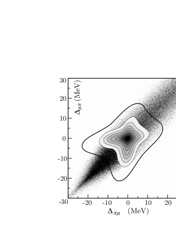
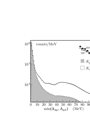
Figure 2: Left: $\Delta_{\mu\pi}$ versus $\Delta_{\pi\mu}$ distribution from MC. $K_{L}$ $\rightarrow$$\pi\mu\nu$ (gray scale) and background (black points). The outsermost contour shows the accepted region. Right: $min(\Delta_{\pi\mu},\Delta_{\mu\pi})$ for data (black dots), MC (solid line), and MC signal (gray shaded histogram).

The right panel of Fig. 2 shows the distribution of the lesser between $\Delta_{\pi\mu}$ and $\Delta_{\mu\pi}$ for data and MC. After the kinematic cuts described above, the contamination, dominated by $K_{L}$$\rightarrow$$\pi e\nu$ decays is $\sim$4%.

To further reduce $K_{L}$$\rightarrow$$\pi e\nu$ background we use the particle identification (PID) based on calorimeter information. Tracks are required to be associated with EMC clusters. We define two variables: $d_{\mathrm{TC}}$, the distance from the extrapolated track entry point in the calorimeter to the cluster centroid and $d_{\perp,\,\mathrm{TC}}$, the component of this distance in the plane orthogonal to the track momentum at the calorimeter entry point.

We accept tracks with $d_{\perp,\,\mathrm{TC}}$ $<$ 30 cm. The cluster efficiency is obtained from the MC, corrected with the ratio of data and MC efficiencies obtained from control samples. These samples, of 86% and 99.5% purity, are obtained from $K_{\mu 3}$ and $K_{e3}$ events selected by means of kinematics and independent calorimeter information. The cluster efficiency correction versus $E_{\nu}$ is shown in Fig. 3.

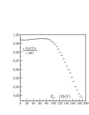
Figure 3: Cluster efficiency correction versus $E_{\nu}$.

For each $K_{L}$ decay track with an associated cluster we define the variable: $\Delta t_{i}=t_{\rm cl}-t_{i},\ (i=\pi,\ e)$ in which $t_{\rm cl}$ is the cluster time and $t_{i}$ is the expected time of flight, evaluated using the corresponding mass. $t_{i}$ includes the time from the entry point to the cluster centroid [18]. We determine the $e^{+}e^{-}$ collision time, $t_{0}$, using the clusters from the $K_{S}$.

The mass assignment,$\pi e$ or $e\pi$, is obtained by choosing the lesser of $|\Delta t_{\pi^{+}}-\Delta t_{e^{-}}|$ and $|\Delta t_{\pi^{-}}-\Delta t_{e^{+}}|$. After the mass assignment has been made, we consider the variable

$$R_{\rm TOF}=\left(\frac{\Delta t_{\pi}+\Delta t_{e}}{2\sigma_{+}}\right)^{2}+\left(\frac{\Delta t_{\pi}-\Delta t_{e}}{2\sigma_{-}}\right)^{2}$$

where $\sigma_{+}$ ($\sigma_{-}$) = $0.5(0.4)$ ns are the resolutions.

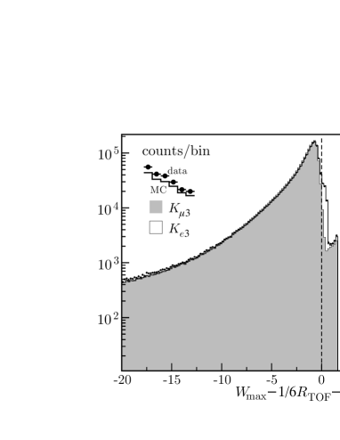
Figure 4: Distribution of $W_{\rm max}$ -1/6$R_{\rm TOF}-0.4$ for data (dots), MC (solid line) and MC signal (gray scale). The dashed line indicates the cut that we use.

Additional information is provided by the energy deposition in the calorimeter and the cluster centroid depth. These quantities are input to a neural network (NN). We retain events with $W_{\rm max}<(1/6)\,R_{\rm TOF}+0.4$, where $W_{\rm max}$ is the largest of the NN outputs for the two charge hypothesis. The distribution of $W_{\rm max}$ -1/6$R_{\rm TOF}-0.4$ for data and MC is shown in Fig. 4. The resulting purity of the sample is $\sim\,97.5\%$, almost uniform in range 16$<E_{\nu}<$181 MeV used for the fit.

The FF parameters are obtained by fitting the $E_{\nu}$ distribution of the selected events in the range $16<E_{\nu}<181$ MeV, subdivided in 32 equal width bins. The bin size,  5 MeV, is about 1.7 times the neutrino energy resolution. The value of $E_{\nu}$, i.e. the missing momentum in the $K_{L}$ rest frame, is determined with a resolution ofabout 3 MeV almost independently on its value. The purity of the final sample used to extract the form factor parameters is illustrated in Fig. 5.

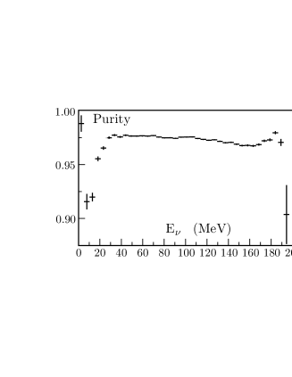
Figure 5: Purity versus $E_{\nu}$.

After subtracting the residual background as estimated from MC, we perform a $\chi^{2}$ fit to the data using the following expression for the expected number of events in each of the 32 bins:

 

$${N_{i}}$$

  (9)

where $\Delta\Gamma_{j}(\mbox{{$\lambda$}})$ is the fraction of events expected for the parameter set defined by $\lambda$ in the $j^{th}$ bin, and $A_{ij}$ is the resolution smearing matrix. $F_{FSR}$ is the final state radiation correction. It is evaluated using the MC simulation, GEANFI  [19], where radiative processes are simulated according the procedures described in Ref. [20]. FSR affects $E_{\nu}$-distribution mainly for high $E_{\nu}$ values, where the correction is about 2%. The free parameters in the fit are the FFs $\lambda$. $N_{0}$ , the total number of signal events, is fixed.

4 Systematic uncertainties

The systematic errors due to the evaluation of corrections, data-MC inconsistencies, result stability, momentum mis-calibration, and background contamination are summarized in Tab. 1, for the case of a quadratic $\tilde{f}_{+}(t)$ and a linear $\tilde{f}_{0}(t)$ .

Source	$\delta\mbox{$\lambda^{\prime}_{+}$}\times 10^{3}$	$\delta\mbox{$\lambda^{\prime\prime}_{+}$}\times 10^{3}$	$\delta\mbox{$\lambda_{0}$}\times 10^{3}$
Tracking	1.60	0.47	0.86
Clustering	2.07	0.61	1.87
TOF + NN	2.23	1.16	1.45
p-scale	1.10	0.71	0.81
p-resolution	0.61	0.21	0.01
Total	3.66	1.58	2.64

Table 1: Summary of systematic uncertainties on $\lambda^{\prime}_{+}$, $\lambda^{\prime\prime}_{+}$, $\lambda_{0}$.

The uncertainty on the tracking efficiency correction is dominated by sample statistics and by the variation of the results observed using different criteria to identify tracks from $K_{L}$ decays. Its statistical error is taken into account in the fit. We study the effect of differences in the resolution with which the variable $d_{\mathrm{c}}$ is reconstructed in data and in MC, and the possible bias introduced in the selection of the control sample, by varying the values of the cuts made on this variable when associating tracks to $K_{L}$ vertexes. For each variation, corresponding to a maximal change of the tracking efficiency of about $\pm$10%, we evaluate the complete tracking-efficiency correction and measure the slope parameters. We observe changes of 1.60$\times 10^{-3}$, 0.47$\times 10^{-3}$, and 0.86$\times 10^{-3}$ for $\lambda^{\prime}_{+}$  $\lambda^{\prime\prime}_{+}$ and $\lambda_{0}$ , respectively.

As for tracking, we evaluate the systematic uncertainties on the clustering efficiency corrections by checking stability of the result when the track-to-cluster association criteria are modified. The statistical uncertainty on the clustering efficiency corrections is taken into account in the fit. The most effective variable in the definition of track-to-cluster association is the transverse distance, $d_{\perp,\,\mathrm{TC}}$. We vary the cut on $d_{\perp,\,\mathrm{TC}}$ in a wide range from 15 cm to 100 cm, corresponding to a change in efficiency of about 19%. For each value of the cut, we obtain the complete track extrapolation and clustering efficiency correction and we use it to evaluate the slopes. We observe changes of 2.07$\times 10^{-3}$, 0.61$\times 10^{-3}$ and 1.87$\times 10^{-3}$ for $\lambda^{\prime}_{+}$ $\lambda^{\prime\prime}_{+}$  and $\lambda_{0}$, respectively.

We study the uncertainties of the efficiency and of the background evaluation by studying the stability of the result with modified PID and kinematic cut values, corresponding to a variation of the cut efficiency from 90% to 95%. This changes the background contamination from 1.5% to 4.5%. We observe changes of 2.23$\times 10^{-3}$, 1.16$\times 10^{-3}$ and 1.45$\times 10^{-3}$ for $\lambda^{\prime}_{+}$ $\lambda^{\prime\prime}_{+}$  and $\lambda_{0}$, respectively.

We also consider the effects of uncertainties in the absolute momentum scale and momentum resolution. A momentum scale uncertainty of 0.1% [19] corresponds to changes of $1.1\times 10^{-3}$, $0.71\times 10^{-3}$, and $0.81\times 10^{-3}$ for $\lambda^{\prime}_{+}$, $\lambda^{\prime\prime}_{+}$, and $\lambda_{0}$, respectively. We investigate momentum resolution effects by changing the value of the resolution on $E_{\nu}$ by 0.1 MeV, an amount which characterizes our knowledge of the momentum resolution, as described in Ref. [4]. We observe changes of $0.61\times 10^{-3}$, $0.21\times 10^{-3}$, and $0.01\times 10^{-3}$ for $\lambda^{\prime}_{+}$, $\lambda^{\prime\prime}_{+}$, and $\lambda_{0}$, respectively.

5 Results and interpretation

About 1.8 million $K_{\mu 3}$ decays were accepted. We first fit the data using Eqs. (2) and (5) for the vector and scalar FFs. The result of this fit is shown in Fig. 6.

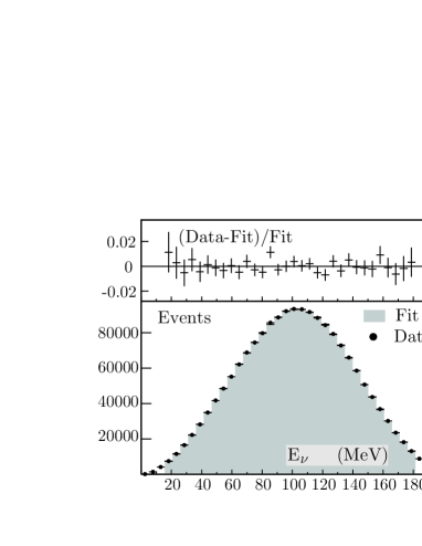
Figure 6: Residuals of the fit (top plot) and $E_{\nu}$ distribution for data events superimposed on the fit result (bottom plot).

We obtain:
$\lambda^{\prime}_{+}$ $\displaystyle=$ $\displaystyle(22.3\pm 9.8_{\rm{stat}}\pm 3.7_{\rm{syst}})\times\rm{10^{-3}}$ $\lambda^{\prime\prime}_{+}$ $\displaystyle=$ $\displaystyle(4.8\pm 4.9_{\rm{stat}}\pm 1.6_{\rm{syst}})\times\rm{10^{-3}}$ $\displaystyle\lambda_{0}$ $\displaystyle=$ $\displaystyle(9.1\pm 5.9_{\rm{stat}}\pm 2.6_{\rm{syst}})\times\rm{10^{-3}}$
       $$\left(\begin{array}[]{ccc}1&-0.97&0.81\\ &1&-0.91\\ &&1\\ \end{array}\right)$$
with $\chi^{2}/{\rm dof}=19/29$, and correlation coefficients as given in the matrix.

Improved accuracy is obtained by combining the above results with those from our $K_{e3}$ analysis[4]:

$$\lambda^{\prime}_{+} = (25.5\pm 1.5_{\rm{stat}}\pm 1.0_{\rm{syst}})\times\rm{10^{-3}}$$

$$\lambda^{\prime\prime}_{+} = (1.4\pm 0.7_{\rm{stat}}\pm 0.4_{\rm{syst}})\times\rm{10^{-3}}$$

We then find:
$\lambda^{\prime}_{+}$ $\displaystyle=$ $\displaystyle(25.6\pm 1.5_{\rm{stat}}\pm 0.9_{\rm{syst}})\times\rm{10^{-3}}$ $\lambda^{\prime\prime}_{+}$ $\displaystyle=$ $\displaystyle(1.5\pm 0.7_{\rm{stat}}\pm 0.4_{\rm{syst}})\times\rm{10^{-3}}$ $\displaystyle\lambda_{0}$ $\displaystyle=$ $\displaystyle(15.4\pm 1.8_{\rm{stat}}\pm 1.3_{\rm{syst}})\times\rm{10^{-3}}$ $$\left(\begin{array}[]{ccc}1&-0.95&0.29\\ &1&-0.38\\ &&1\\ \end{array}\right)$$
with $\chi^{2}/{\rm dof}=2.3/2$ and the correlations given in the matrix on the right.

Finally, to take advantage of the recent parameterizations of the FFs based on dispersive representations (Eqs. (4) and (7)), we combine our results from this analysis of $K_{\mu 3}$ data with our previous result for $K_{e3}$. We perform a fit to the values obtained for $\lambda^{\prime}_{+}$, $\lambda^{\prime\prime}_{+}$, and $\lambda_{0}$ that makes use of the total error matrix as described above, and the constraints implied by Eqs. (1) and (8). Thus, the vector and scalar FFs are each described by a single parameter. Dropping the “$\;{}^{\prime}\;$” notations, we find

$$\lambda_{+} = (25.7\pm 0.4_{\rm{stat}}\pm 0.4_{\rm{syst}}\pm 0.2_{\rm{param}})\times\rm{10^{-3}}$$

$$\lambda_{0} = (14.0\pm 1.6_{\rm{stat}}\pm 1.3_{\rm{syst}}\pm 0.2_{\rm{param}})\times\rm{10^{-3}}$$

with $\chi^{2}/{\rm dof}=2.6/3$ and a total correlation cofficient of $-0.26$. The uncertainties arising from the choice of parameterization for the vector and scalar FFs are $0.2\times 10^{-3}$ and $0.1\times 10^{-3}$ using only $K_{e3}$ decays and $K_{\mu 3}$ decays, respectively. These contributions to the uncertainty on $\lambda_{+}$ and $\lambda_{0}$ are explictly given in Eq. (5). We note that the use of Eq. (8) changes the value of the phase space integral by only 0.04% with respect to the result obtained using a linear parameterization for $\tilde{f}_{0}(t)$.

Finally, from the Callan-Treiman relation we compute $f(0)=0.964\pm 0.023$ using $f_{K}/f_{\pi}=1.189\pm 0.007$ from Ref. [21]. Our value for $f(0)$ is in agreement with the results of recent lattice calculations [22].

6 Conclusions

We have performed a new measurement of the $K_{L}\rightarrow\pi\mu\nu$ FFs. Our results are in acceptable agreement with the measurements from KTeV [2] and ISTRA+ [10] and in disagreement with those from NA48 [9, 3]. In particular, our result for the scalar FF parameter $\lambda_{0}=0.0143\pm 0.00203$ (Eq. (5)) accounts for the presence of a $t^{2}$ term. KTeV and ISTRA+ use a linear parameterization; as a consequence, their values for $\lambda_{0}$ are systematically high by $\sim$0.003. We also derive $f^{K^{0}}(0)=0.964\pm 0.023$. This value is in agreement with the results of recent lattice calculations [22].

Appendix A Error estimates

It is quite easy to estimate the ideal error in the measurements of a set of parameters p=$(p_{1},\>p_{2},\ldots\>p_{n})$ from fitting some distribution function to experimentally determined spectra. Let $F(\mathbf{p},x)$ be a probability density function, PDF, where ${\mathbf{p}}$ is some parameter vector, which we want to determine and $x$ is a running variable, like $t$. The inverse of the covariance matrix for the maximum likelihood estimate of the parameters is given by [23]:

$$({\bf G}^{-1})_{ij}=-{\partial^{2}\ln L\over\partial p_{i}\partial p_{j}}$$

from which, for $N$ events, it trivially follows:

$$\left({\bf G}^{-1}\right)_{ij}=N\>\int{1\over F}\,{\partial F\over\partial p_{i}}\,{\partial F\over\partial p_{j}}\>\hbox{d}\upsilon,$$

with $\hbox{d}\upsilon$ the appropriate volume element. We use in the following the above relation to estimate the errors on the FF parameters for one and two parameters expression of the FFs $\tilde{f}_{+}(t)$ and $\tilde{f}_{0}(t)$. The errors in any realistic experiment will be larger than our estimates, typically two to three times. The above estimates are useful for the understanding of the problems in the determination of the parameters in question.

A.1 $K_{e3}$ decays

For a quadratic FF, $\tilde{f}(t)=1+\mbox{$\lambda^{\prime}_{+}$}(t/m^{2})+(\mbox{$\lambda^{\prime\prime}_{+}$}/2)(t/m^{2})^{2}$, the inverse of the covariance matrix ${\bf G}_{+}^{-1}$, the covariance matrix ${\bf G}_{+}$ and the correlation matrix are:

$$N\,\pmatrix{5.937&13.867\cr\vglue-11.38109pt\cr\cr 13.867&36.2405\cr},\kern 14.22636pt{1\over N}\,\pmatrix{1.258^{2}&-0.606\cr\vglue-11.38109pt\cr\cr-0.606&0.509^{2}},\kern 14.22636pt\pmatrix{1&-.945\cr\vglue-11.38109pt\cr\cr&1\cr}$$

The square root of the diagonal elements of ${\bf G}_{+}$ gives the errors, which for one million events are $\delta\lambda_{+}^{\prime}$=0.00126, $\delta\lambda_{+}^{\prime\prime}$=0.00051. The correlation is very close to $-$1, meaning that, because of statistical fluctuation of the bin counts, a fit will trade $\lambda^{\prime}_{+}$ for $\lambda^{\prime\prime}_{+}$ and that the errors are enlarged. A fit for a linear FF, $\tilde{f}(t)=1+\mbox{$\lambda^{\prime}_{+}$}(t/m^{2})$ in fact gives $\lambda^{\prime}_{+}$=0.029 instead of 0.025 and an error smaller by $\sim$3:

$$\hbox{$\delta\lambda_{+}^{\prime}$}=\sqrt{{\bf G}_{+}(1,1)}=0.0004.$$

A simple rule of thumb is that ignoring a $t^{2}$ term, increases $\lambda^{\prime}_{+}$ by $\sim$3.5$\times$$\lambda^{\prime\prime}_{+}$. For $K_{e3}$ decays the presence of a $t^{2}$ term in the FF is firmly established. It is however not fully justified to fit for two parameters connected by the simple relation $\lambda^{\prime\prime}_{+}$=2$\times$$\lambda^{\prime}_{+}$². The authors of ref. 6, 7 explicitly give an error for their estimate of the coefficient of the $t^{2}$ terms. The above discussion justifies the use of eq. 1. The errors obtained above compare reasonably with the errors quoted in [2, 3, 4], when all experimental problems are taken into account.

A.2 $K_{\mu 3}$ decays

The scalar FF only contributes to $K_{\mu 3}$ decays. Dealing with these decays is much harder because: a) - the branching ratio is smaller, resulting in reduced statistics, b) - the $E_{\pi}$ or $t$ range in the decay is smaller, c) - it is in general harder to obtain an undistorted spectrum and d) - more parameters are necessary. This is quite well evidenced by the wide range of answers obtained by different experiments [2, 10, 9]. Assuming that both scalar and vector FF are given by quadratic polynomials as in eq. 2, ordering the parameters as $\lambda^{\prime}_{0}$, $\lambda^{\prime\prime}_{0}$, $\lambda^{\prime}_{+}$ and $\lambda^{\prime\prime}_{+}$, the matrices ${\bf G}_{0\,\&\,+}^{-1}$ and ${\bf G}_{0\,\&\,+}$, are:

$$N\pmatrix{1.64&5.44&1.01&3.90\cr\vglue-11.38109pt\cr\cr 5.44&18.2&3.01&12.3\cr\vglue-11.38109pt\cr\cr 1.01&3.01&1.47&4.24\cr\vglue-11.38109pt\cr\cr 3.90&12.3&4.24&13.8\cr},\ {1\over N}\pmatrix{63.9^{2}&-1200&-923&197\cr\vglue-11.38109pt\cr\cr-1200&18.8^{2}&272&-59\cr\vglue-11.38109pt\cr\cr-923&272&14.8^{2}&-49\cr\vglue-11.38109pt\cr\cr 197&-59&-48&3.4^{2}\cr}$$

and the correlations, ignoring the diagonal terms, are:

$$\pmatrix{-0.9996&-0.974&0.91\cr\vglue-11.38109pt\cr\cr&0.978&-0.919\cr\vglue-11.38109pt\cr\cr&&-0.976\cr}.$$ (10)

All correlations are very close to $-$1. In particular the correlations between $\lambda^{\prime}_{0}$ and $\lambda^{\prime\prime}_{0}$ is $-$99.96%, reflecting in vary large $\delta\lambda_{0}^{\prime}$ and $\delta\lambda_{0}^{\prime\prime}$ errors. We might ask what the error on $\lambda^{\prime}_{0}$ and $\lambda^{\prime\prime}_{0}$ might be if we had perfect knowledge of $\lambda^{\prime}_{+}$ and $\lambda^{\prime\prime}_{+}$. The inverse covariance matrix is give by the elements (1,1), (1,2), (2,1) and (2,2) of the ${\bf G}_{0\,\&\,+}^{-1}$ matrix above. The covariance matrix therefore is :

$${\bf G}_{0}(\mbox{$\lambda^{\prime}_{0}$},\ \mbox{$\lambda^{\prime\prime}_{0}$}\ \hbox{for \mbox{$\lambda^{\prime}_{+}$}, \mbox{$\lambda^{\prime\prime}_{+}$}\ known})={1\over N}\pmatrix{8.2^{2}&-20\cr\cr\vglue-11.38109pt\cr-20&2.4^{2}\cr}.$$

For one million events we have $\delta\lambda_{0}^{\prime\prime}$=0.0024, about 4$\times$ the expected value of $\lambda^{\prime\prime}_{0}$. In other words $\lambda^{\prime\prime}_{0}$ is likely to be never measurable. It is however a mistake to assume a scalar FF linear in $t$, because the coefficient of $t$ will absorb the coefficient of a $t^{2}$ term, again multiplied by $\sim$3.5. Thus a real value $\lambda^{\prime}_{0}$=0.014 is shifted by the fit to 0.017, having used eq. 8. Fitting the pion spectrum from 1 million $K_{\mu 3}$ decays for $\lambda_{0}$, $\lambda_{+}$ with the FFs of eq. 8 and 1 gives the errors $\delta\lambda_{0}^{\prime}$$\sim$0.0096 and $\delta\lambda_{+}^{\prime}$$\sim$0.00097. Combining with the result from a fit to 1 million $K_{e3}$ with the FF of eq. 1 for which $\delta\lambda_{+}^{\prime}$$\sim$0.00037 gives finally $\delta\lambda_{0}^{\prime}$$\sim$0.00075, $\delta\lambda_{+}^{\prime}$$\sim$0.00034 and a $\lambda_{0}$-$\lambda^{\prime}_{+}$ correlation of $-$31%. Using the neutrino spectrum for $K_{\mu 3}$ decays, the errors are only slightly larger: $\delta\lambda_{0}^{\prime}$$\sim$0.001, $\delta\lambda_{+}^{\prime}$$\sim$0.00036. We hope to reach this accuracy with our entire data sample, $\sim$5$\times$ the present one, and a better analysis which would allow using the pion spectrum.

References

[1]
[2]
T. Alexopolous et al. [KTeV Collaboration], Phys. Rev. D 70 (2004) 092007.
[3]
A. Lai et al. [NA48 Collaboration], Phys. Lett. B 606 (2004) 1.
[4]
F. Ambrosino et al. [KLOE Collaboration], Phys. Lett. B 636 (2006) 166.
[6] V. Bernard, M. Oertel, E. Passemar and J. Stern, Phys. Lett. B 638 (2006) 480
[7] V. Bernard, M. Oertel, E. Passmar and J. Stern, private communication. They compute a dispersion relation for ln twice subtracted at , using P-wave scattering data, as done in [6].
[8] M. Jamin, A. Pich and J. Portoles, Phys. Lett. B 640 (2006) 176
[9]
A. Lai et al. [NA48 Collaboration], Phys. Lett. B 647 (2007) 341.
[10]
O. P. Yushchenko et al., Phys. Lett. B 581 (2004) 31.
[11]
C. G. Callan, S. Treiman, Phys. Rev. Lett. 16 (1966) 153.
[12]
J. Gasser, H. Leutwyler, Nucl. Phys. B 250 (1985) 93.
[13] M. Jamin, J. A. Oller and A. Pich, Phys. Rev. D 74 (2006) 074009
[14]
M. Adinolfi et al. [KLOE Collaboration], Nucl. Instrum. Meth. A 488 (2002) 51.
[15]
M. Adinolfi et al. [KLOE Collaboration], Nucl. Instrum. Meth. A 482 (2002) 364.
[16]
M. Adinolfi et al. [KLOE Collaboration], Nucl. Instrum. Meth. A 492 (2002) 134.
[17]
F. Ambrosino et al. [KLOE Collaboration], Phys. Lett. B 632 (2006) 43;
M. Antonelli, P. Beltrame, M. Dreucci, M. Moulson, M. Paultan, A. Sibidanov,
Measurements of the Absolute Branching Ratios for Dominant Decays, the
Lifetime, and with the Kloe Detector, KLOE Note 204 (2005).
http://www.lnf.infn.it/kloe/pub/knote/kn204.ps.gz
[18]
F. Ambrosino et al. [KLOE Collaboration], Phys. Lett. B 636 (2006) 173, and
references therein.
[19]
F. Ambrosino et al. [KLOE Collaboration], Nucl. Instrum. Meth. A 534 (2004) 403.
[20]
C. Gatti, Eur. Phys. J. C, 45 (2006) 417.
[21]
E. Follana et al. arXiv:0706.1726 [hep-lat] (2007).
[22]
D. Becirevic et al.,
Nucl. Phys. B 705, 339 (2005);
M. Okamoto [Fermilab Lattice, MILC and HPQCD Collaborations],
Int. J. Mod. Phys. A 20, 3469 (2005);
N. Tsutsui et al. [JLQCD Collaboration],
PoS LAT2005, 357 (2006)
[arXiv:hep-lat/0510068];
C. Dawson, T. Izubuchi, T. Kaneko, S. Sasaki and A. Soni,
Phys. Rev. D 74, 114502 (2006);
D. J. Antonio et al.,
arXiv:hep-lat/0702026.
[23] H. Cramer, Mathematical Methods of Statistics, Princeton University Press,
1946, proves that this is the smallest possible error.