PUTP-2240

Holographic flavor in theories with eight supercharges

Diego Rodríguez-Gómez

Joseph Henry Laboratories, Princeton University

Princeton NJ 08544, U.S.A.

drodrigu@princeton.edu

ABSTRACT

We review the holographic duals of gauge theories with eight supercharges obtained by adding very few flavors to pure supersymmetric Yang-Mills with sixteen supercharges. Assuming a brane-probe limit, the gravity duals are engineered in terms of probe branes (the so-called flavor brane) in the background of the color branes. Both types of branes intersect on a given subspace in which the matter is confined. The gauge theory dual is thus the corresponding flavoring of the gauge theory with sixteen supercharges. Those theories have in general a non-trivial phase structure; which is also captured in a beautiful way by the gravity dual. Along the lines of the gauge/gravity duality, we review also some of the results on the meson spectrum in the different phases of the theories.

1 Introduction

Gauge theories are the cornerstone of our current understanding of Nature. The Standard Model is, with no doubt, the most successful model of Nature we have so far constructed. It incorporates, under the unified framework of Quantum Field Theory, the electroweak and the strong interactions, being both gauge theories. However, there is yet another force of Nature, gravity, which is left apart in this scheme. String Theory is the most promising candidate for a unified theory, in which gauge and gravity are two sides of the same coin. Along this lines, the gauge/gravity correspondence [1] (see [2] for a very comprehensive review) has been a breakthrough in our understanding of both gravity (and string theory) and gauge field theories. This correspondence provides a closed string description, based on classical supergravity, of the dynamics of gauge theories at large ’t Hooft coupling. It deeply relies on the dual description of gravitational objects either as backgrounds on which strings propagate; and as objects on its own right in the theory. The most celebrated example considers the very special case of the $D3$ branes, which can be seen either as a certain supergravity background, or as an object which carries a worldvolume gauge theory as the lowest lying states. In a well-defined low energy limit, namely the decoupling limit, changing from weak to strong coupling takes us from one description to the other. This duality is indeed a holographic duality [3, 4, 5], since the weak coupling is described in terms of a field theory living in four-dimensional Minkowski, whereas the strong coupling is captured in terms of IIB string theory propagating in ten-dimensional $AdS_{5}\times S^{5}$ (which is the near horizon region of the $D3$ brane background, on which the decoupling limit focuses). In a sense, it captures the original spirit of string theory as an effective description of the strong coupling regime of a gauge theory.

Many avenues of the gauge/gravity duality have been explored by now. The dictionary between both sides has been established (see [2] and references therein), and many more examples have been found (see also [2, 6, 7, 8, 9]). Technically, the duality works in its most stelar way for $AdS$ backgrounds, whose field theory duals are in terms of supersymmetric conformally invariant field theories. This is inherited from the structure of the $AdS$ space, which endows the holographic dual theory with a conformal invariance. Restricting for a while to $3+1$ dimensions, in principle one can find dualities for spaces of the form $AdS_{5}\times X$, as long as $X$ is a five-dimensional Sasaki–Einstein manifold. This has been done in the literature, where both the gravity and field theory sides have been explicitly worked out, finding an amusing agreement (see [6, 7, 8, 9] and references to those papers). These backgrounds can be seen as the near horizon limit for $D3$ branes at the tip of the Calabi–Yau cone whose base is the $X$ space. This cone is, in general, singular (although the near horizon removes this singularity), and one can desingularize it by moving in the Kahler moduli space resolving the singularities [10, 11]. This has also been studied, leading to a deeper understanding of the interplay geometry/gauge theory. However, understanding the breaking of conformal invariance in this context remains as a major challenge, since the ultimate challenge is to understand in a holographic way a theory such as QCD. A major step was taken in [12], where, by introducing fractional branes which in turn require deforming the conifold (which amounts to moving along the complex structure moduli space of the internal Calabi–Yau), the conformal invariance was broken and the dual of a confining gauge theory was found.

Going back to the original spirit of the gauge/gravity duality, one could try to play the same game not just for the $D3$ brane, but for a generic $Dp$ [14, 13]. In the general case the situation is very different, since, once one finds the suitable holographic coordinates, the gravity dual lives in a background which is not $AdS$, but only conformally $AdS$. Since in addition in these backgrounds the dilaton is not constant, the conformal invariance of the dual theory is broken; which makes the duality somehow more subtle, and valid just in a certain energy and parameter range. Since the dilaton will be a function of the holographic coordinate; which in turn has the interpretation of the energy scale in the dual theory, generically we will have that, for some energy range, the gravity dual opens up the M-theory circle. In a suitable parameter range, this corresponds in the field theory to a strong coupling regime, which we can surpass by uplifting the system to 11 dimensions. However, taking into account all these subtleties, one can still formulate a gauge/gravity duality for the generic case of $Dp$ branes.

In the dual field theories discussed, all fields are in the adjoint representation. Clearly, a major issue is to introduce matter (quarks) in the fundamental representation, and this will be precisely our main interest. Our ultimate goal in this paper will be to understand the dynamics of a certain class of gauge theories with flavors which admit a gravity description. Those theories will arise as the flavoring of a “bulk” Yang–Mills with 16 supercharges in $p+1$ dimensions. In order to find the bulk theories, we will restrict from now on to the case in which those $Dp$ branes live in ten-dimensional Minkowski space. Therefore, the field theory description will be in terms of the worldvolume theory on the branes; which is precisely the aforementioned bulk theory. To be more precise, we will be interested in adding fundamental matter to the gauge theories obtained from dimensional reduction of the maximally supersymmetric Yang–Mills theory in ten dimensions down to $p+1$. Indeed, we will consider adding supersymmetrically $N_{f}$ hypermultiplets to those theories in all the possible ways (namely confined to live inside a defect of the various dimensionalities selected by supersymmetry).

Adding fundamental matter is equivalent to introducing open string degrees of freedom to the supergravity side of the correspondence, and can be achieved by adding $D$-branes to the supergravity background. A first step towards the addition of an open string sector was taken in [15, 16, 17, 18, 19, 20, 21], where it was suggested that one can have dynamical open string degrees of freedom by introducing $N_{f}$ intersecting $Dq$ branes to the original $Dp$ branes. In the limit in which the number of $Dq$ branes is much smaller than the number of $Dp$ branes, we can treat the system effectively as $N_{f}$ probe branes in the background generated by the $N_{c}$ $Dp$ branes. Thus, once we take the decoupling limit, this background will reduce to the corresponding near horizon geometry of the original $Dp$ branes, where the $Dq$ live embedded as probes. Generically, the two types of branes overlap partially, which implies that the additional $Dq$ branes create a defect on the worldvolume theory of the $Dp$ branes. In the dual gauge theory description, the extra branes give rise to additional matter, confined to live inside the defect, which comes from the $Dp-Dq$ strings. When $q>p$, the decoupling limit forces the $SU(N_{f})$ gauge symmetry on the $Dq$ brane to decouple. It then appears as a global flavor symmetry for the extra matter, which is in the fundamental representation of the flavor group; furnishing precisely the type of field theories which we wanted to study. Although we will restrict to the aforementioned theories (namely $p+1$ Yang–Mills with 16 supercharges containing a few flavors confined in a half-BPS defect), this approach to the flavor problem can be used in a generic way. In this context, the fluctuations of the flavor branes should correspond to the mesons in the dual gauge theory. The study of these mesons was started in [22] for the $D7$ brane in the $AdS_{5}\times S^{5}$ geometry, and it was further extended to other flavor branes in several backgrounds [23, 24, 25, 26, 27, 28, 29, 30, 31, 32, 33, 34, 35, 36, 37, 38, 39, 40, 41, 42, 43, 44, 45, 46, 47, 48, 49, 50, 51, 52, 53, 54] (for a review see [55]). From the field theory point of view, this approach is some sort of quenched approximation, since the backreaction of the flavors on the color is not taken into account. It is just since very recently that a full approach to the problem has been considered with very interesting results (see [56, 57, 58, 59, 60, 61, 62]).

Our purpose is to present a compilation of the accumulated results which describe the gauge/gravity duality for the theories of interest. We first start introducing the gauge/gravity duality which will be the arena of our discussion. Inspired by the $AdS/CFT$ correspondence, whose biggest exponent is the $AdS_{5}/{\cal{N}}=4$ duality, we discuss a bit the duality for the rest of $Dp$ branes. An exhaustive description of each case is, by far, out of the scope of this paper, and we refer to the literature (in particular see [2] and references therein) for deeper discussions. After introducing the gauge/gravity duality we turn to the inclusion of fundamental matter along the lines of [15, 16, 17, 18, 19, 20, 21]. The bottom line is that, in the brane-probe approximation, the flavor is included as probes in the color branes background, where we have to take the gauge/gravity duality and go to the “near horizon” region of the space as dual of the gauge theory. However, the addition of the flavor branes is somehow subtle. Since here we are mainly interested in supersymmetric field theories, our first task will be to find the supersymmetric embeddings for the probes; which will give rise to three series of intersections characterized by the codimensionality of the defect in the color branes: codimension 0, codimension 1 and codimension 2. We will see in the next section that, as long as we do not consider worldvolume gauge fields, the flavor branes do not couple the background RR potential. Actually, in Sec. 2, we review all the intersections in the Coulomb branch from the gravity side in a generic way, paying a special attention to the $D3$ brane background for later purposes. However, at this point, we preferred not to introduce yet the full field theory analysis, and postpone it for later in order to have a more unified picture. The fact of not considering worldvolme gauge fields on the probe branes will have the consequence that this brane embeddings correspond to the Coulomb branch of the theory; whose properties, such as the meson spectrum, will be studied in Sec. 3 by considering the fluctuations of the flavor branes. This was first studied in [22] for the $D3-D7$ case and subsequently extended to the other brane intersections in [52] and [53] (for a review see [55]).

We can have more involved situations in the field theory, such as Higgs branches. We turn to them in Sec. 4. Since the $D3$ brane background has special properties, such as the conformality of the bulk ${\cal{N}}=4$ Yang–Mills theory and the fact that it is $(3+1)$-dimensional, we will study the three intersections whose background is that of the $D3$ brane in more detail using them as examples for the rest of the intersections. Indeed, we will take advantage of the gained perspective when studying the Coulomb branch of the theory to discuss in detail, from the field theory point of view, the dynamics of the systems. We will see that the field theory results have a beautiful gravity counterpart. We start with the codimension 0 defect. For the particular $D3-D7$ case, the Higgs phase was first studied in [63] (see also [64] and [65]). It was proposed in [63] and [64] that, from the point of view of the $D7$-brane, one can realize a (mixed Coulomb–)Higgs phase of the $D3-D7$ system by switching on an instanton configuration of the worldvolume gauge field of the $D7$-brane. This instanton has the effect of separating some of the color branes and dissolving them in the flavor ones since it couples to the flavor branes the background potential. Heuristically this explains why this corresponds to a Higgs branch. Since we are separating some of the color branes, the gauge group is broken; and the fact of dissolving (recombining) them with the flavor ones has the effect of giving a nontrivial VEV for the quark fields, thus entering into the Higgs branch. This picture will be universal for both the codimension 0 and codimension 1 defects; and is shared by other approaches to the same gauge theories (such as brane webs. For a review see [66]. It was also suggested in [67]). We will see that one can give a very explicit realization of these ideas from the perspective of the “separated branes,” which can be thought as moving in the background of the rest. Because of the dielectric effect [68], they will polarize into the effective flavor brane, giving a precise and beautiful relation between the field theory and the gravity pictures.

We then turn to the codimension 1 defect. In this case we will study in detail the $D3-D5$ intersection, which is dual to an ${\mathcal{N}}=1$ three-dimensional defect living in a bulk ${\mathcal{N}}=4$ four-dimensional gauge theory. The field theory was extensively studied in [69] and [70], as well as some aspects of the brane construction in the Coulomb phase. The corresponding Higgs phase for this intersection was discussed in [71]. On the field theory side the $D3-D5$ system describes the dynamics of a $(2+1)$-dimensional defect containing fundamental hypermultiplets living inside the $(3+1)$-dimensional ${\cal{N}}=4$ SYM. The meson spectra on the Coulomb branch was extensively studied in [52]. In [71] it was found that, in the supergravity dual, the Higgs phase also corresponds to adding magnetic worldvolume flux inside the flavor $D5$-brane transverse to the $D3$-branes. This worldvolume gauge field has the nontrivial effect of inducing $D3$-brane charge in the $D5$-brane worldvolume (which reflects the recombination of some of the color $D3$ with the flavor $D5$), which in turn suggests an alternative microscopical description in terms of $D3$-branes expanded to a $D5$-brane due to dielectric effect [68] along the same lines as in the $D3-D7$ case.Indeed, the vacuum conditions of the dielectric theory can be mapped to the $F$ and $D$ flatness constraints of the dual gauge theory, thus justifying the identification with the Higgs phase, in very much of the same spirit of what happened in the $D3-D7$ case. In this case, the Higgs vacua of the field theory involve a nontrivial dependence of the defect fields on the coordinate transverse to the defect. In the supergravity side this is mapped to a bending of the flavor brane, which is actually required by supersymmetry (see [72]). Moreover, in [71] the spectrum of transverse fluctuations was computed in the Higgs phase, with the result that the discrete spectrum is lost. The reason is that the IR theory is modified because of the nontrivial profile of the flavor brane, so that in the Higgs phase, instead of having an effective $AdS\times S$ worldvolume for the flavor brane, one has Minkowski space, thus loosing the KK-scale which would give rise to a discretespectrum.

Lastly, we turn to the codimension 2 defect, which behaves rather different from the other intersections. The defect conformal field theory associated to the $D3-D3$ intersection was studied in [73], where the corresponding fluctuation/operator dictionary was established. The meson mass spectra of this system when the two sets of $D3$-branes are separated was computed analytically in [52]. In [73] the Higgs branch of the $D3-D3$ system was identified as a particular holomorphic embedding of the probe $D3$-brane in the $AdS_{5}\times S^{5}$ geometry, which was shown to correspond to the vanishing of the $F$- and $D$-terms in the dual superconformal field theory (see also [74] and [75]). This intersection behaves in a rather different way since the two brane-stacks are of the same dimensionality. Indeed, in this case the flavor symmetry will not decouple as local symmetry; and thus these theories should be understood in a different way.

2 Adding Matter to Gauge/Gravity Duality: BPS Intersections as Holographic Flavor

As we said, a major challenge remains the addition of fundamental matter to the gauge/gravity duality in a fully satisfactory manner. We will consider a first approximation to the problem, in which we will think of the flavors as coming from some brane probes in the background of the branes generating the color degrees of freedom. However, we first review the gauge/gravity correspondence for theories with 16 supercharges. For further details we refer to the original [1] and [14] and the review article [2].

2.1 An overview of gauge/gravity duality

The most celebrated example of gauge/gravity duality is the $AdS/CFT$ correspondence, out of which the major example is the one relating ${\mathcal{N}}=4$ SYM theory in four-dimensional Minkowski to IIB string theory on $AdS_{5}\times S^{5}$. A lot of effort has been put towards understanding this duality and finding an explicit dictionary between gravity and gauge theory. Also, by now, we have infinitely many more examples of dualities between conformal field theories with diverse supersymmetries and IIB string theory on spaces of the form $AdS_{5}\times L^{a,b,c}$. In addition, there are many other examples in other dimensions, whose gravity dual involves various $AdS$ spaces.

In general, the gauge/gravity duality relies on the dual description of branes in a certain limit as supergravity backgrounds or as gauge theories. In the very special case of the $D3$ brane, this duality can be put forward in a very precise manner, and because of the very special properties of the $D3$ brane background (in particular the $AdS_{5}$ near horizon with constant dilaton), a precise $AdS/CFT$ duality can be stated. However, not without a number of subtleties, one can, to some extend, adapt this correspondence to the generic case of $Dp$ branes.

The most celebrated gauge/gravity duality$:$ $AdS/CFT$ for $D3$ branes

Let us consider $N$ $D3$ branes in flat space. Since we want to use a string theory picture, we need to keep the dilaton (or analogously $e^{\Phi}$) small. However, for $D3$ branes, the dilaton is a constant, so we simply have to ensure that the asymptotic value $e^{\Phi_{0}}=g_{s}$ is small. Being massive objects, the $D3$ branes will backreact on the geometry and generate an asymptotically flat space with a horizon at $r=0$

$$ds^{2}=f_{3}^{-\frac{1}{2}}\,dx_{1,3}^{2}+f_{3}^{\frac{1}{2}}(dr^{2}+r^{2}\,d\Omega_{5}^{2})\,,\qquad f_{3}=1+\frac{R^{4}}{r^{4}}\,.$$ (1)

The near horizon region reduces to the $AdS_{5}\times S^{5}$ geometry. The size of the $AdS$ space is given by

$$R^{4}=4\pi g_{s}Nl_{s}^{4}\,,$$ (2)

and it can be thought as the size of the perturbation on the flat space generated by the branes.

We will now take the so-called decoupling limit of $l_{s}\rightarrow 0$ keeping fixed the energy of the excitations. However, energies are measured at infinity, so the precise relation between the proper energy $E_{\rm proper}$ of some excitation and its energy measured at infinity $E$ is

$$E=f_{3}^{-\frac{1}{4}}E_{\rm proper}=\bigg{(}1+\frac{R^{4}}{r^{4}}\bigg{)}^{-\frac{1}{4}}E_{\rm proper}\,.$$ (3)

In the large $r$ asymptotically flat region we have $f_{3}\sim 1$, and therefore the space (1) reduces to ten-dimensional Minkowski. Since $E=E_{\rm proper}$, just the massless excitations (namely the supergravity multiplet) keep a finite energy and survive the limit. On the other hand, in the near horizon region $r\sim 0$, where

$$f_{3}\sim\frac{R^{4}}{r^{4}}\,,$$ (4)

we have that (1) reduces to $AdS_{5}\times S^{5}$. Upon redefining $r=R^{2}z$ we can write its metric as

$$ds^{2}=R^{2}\bigg{(}z^{2}\,dx_{1,3}^{2}+\frac{1}{z^{2}}\,dz^{2}+d\Omega_{5}^{2}\bigg{)}\,.$$ (5)

In addition, in this region we have $E=RzE_{\rm proper}$. Therefore, all the excitations survive the limit since all of them appear asymptotically as low energy modes. Amazingly, this two subsystems are completely decoupled in this limit. Therefore, we can think of the system to be composed of IIB supergravity on ten-dimensional Minkowski plus IIB string theory on $AdS_{5}\times S^{5}$.

In order to trust the description of branes as a supergravity background, we need to have very small curvature in $l_{s}$ units. Since the curvature is proportional to the inverse of the $AdS$ radius ${\mathcal{R}}\sim R^{-1}$, this amounts to require that $l_{s}R^{-1}\ll 1$, so we need to require $g_{s}N$ to be large. In a sense, in this limit we are regarding the branes as a delocalized perturbation of the Minkowski space, and we are replacing them with the geometry (plus RR 5-form flux) they source. Since $g_{s}$ should be small in order to have a perturbative string description, it is clear that we have to take $N$ to be large, so that $g_{s}N\gg 1$.

On the other hand, we can take the opposite limit, namely that in which we regard the system as a stack of localized $D3$ branes in flat Minkowski space. By taking the same limit as before, namely $l_{s}\rightarrow 0$ with fixed energy for the excitations, we just keep the low energy states; which in this case restrict to ${\mathcal{N}}=4$ Yang–Mills theory on the worldvolume of the branes with a fixed and small Yang–Mills coupling $g_{\rm YM}^{2}=2\pi g_{s}$, plus IIB supergravity in the bulk ten-dimensional Minkowski space. In addition, both subsystems are decoupled, and therefore do not talk to each other. Clearly, in order to trust this description, we must have that, away from the branes, the space is not disturbed. In other words, we have to ensure that the typical size of the perturbation of flat space which the branes generate is localized in a small region in $l_{s}$ units; so that we can think of the system as a localized $D3$-brane stack in ten-dimensional Minkowski. This requires $g_{s}N\sim\sqrt{\lambda}$ to be small (here $\lambda$ is the ’t Hooft coupling $\lambda=g_{\rm YM}^{2}N$). Meanwhile, in order to match the dual description, $N$ has to be large. Thus, the dual $SU(N)$ theory is taken at a small Yang–Mills coupling with large $N$, so that $\lambda$ is small. This is the ’t Hooft limit, in which just the planar sector of the gauge theory survives.

Given that we have two descriptions of the same system, and in both of them there is a piece which is the same (namely IIB supergravity excitations around ten-dimensional Minkowski space), it is natural to conjecture following [1] that the remaining subsystems are also equivalent, namely, that IIB strings on $AdS_{5}\times S^{5}$ are dual to ${\mathcal{N}}=4$ SYM.

Let us note that the $AdS/CFT$ duality is a strong/weak coupling duality. The field theory approximation requires the ’t Hooft coupling to be small, whereas in the supergravity side it must be large in order to ensure small curvatures. Thus, increasing $g_{\rm YM}$ takes us from a field theory description to a string theory description.

$AdS$ space, conformal invariance and holography

From the point of view of the decoupling limit, in the gravity side the fixed energies with $l_{s}\rightarrow 0$ are measured asymptotically. This suggests that, in a sense, the dual gauge theory lives in the boundary of the space. Given that the boundary is a lower dimensional space but still the two descriptions carry the same information, the gauge/gravity correspondence is a holographic duality. One way to make this holography more explicit is by considering the Euclidean version of $AdS_{p+1}$, which can be considered as $R^{p+1}$ endowed with the following metric:

$$ds^{2}=\frac{4dy_{i}\,dy_{j}\,\delta^{ij}}{(1-\vec{y}^{2})^{2}}\,.$$ (6)

This space has an $S^{p}$ boundary at $\vec{y}^{2}=1$ where the metric has a double pole and blows up. Because of this double pole, naively one can make sense of the metric just in the interior region. However, we can extend the metric to the boundary provided we allow the metric on the boundary to transform in such a way that it compensates the factor which is blowing up. This endows the boundary with a conformal structure responsible for the conformal invariance of the dual gauge theory. For a wonderful explanation of the deep implications of these facts see [4].

Rotating back to the Lorentz space, one can write the $AdS_{p+1}$ metric as

$$ds^{2}=\frac{dx_{1,p}^{3}+du^{2}}{u^{2}}\,,$$ (7)

which is related to the metric in (1) as $u=z^{-1}$. In this coordinates one can see that scale transformations $x^{\mu}\rightarrow\lambda x^{\mu}$ are a symmetry only if $u\rightarrow\lambda u$. Since scale transformations are linked with $u$ rescalings, it is natural to interpret the radial coordinate in $AdS$ as the energy scale of the theory.

The gauge/gravity correspondence should be provided with a dictionary relating quantities computed in both sides of the duality [4, 5, 76] (see [2, 80] or [81] for reviews on this issues). Exploring this dictionary is, by far, beyond the scope of this work. However, let us mention that, in the gravity side, one expects to have supergravity fluctuations propagating in the $AdS$ space. In general, those fluctuations will be functions of the radial coordinate in $AdS$, and we will typically have two types of behavior near the boundary. Considering a scalar fluctuations for illustrative purposes, if the fields are canonically normalized, the normalizable modes behave at infinity as $\rho^{-\Delta}$, whereas the nonnormalizable ones should behave as $\rho^{\Delta-d-1}$; being $\Delta$ the conformal dimension of the field theory operator associated to the supergravity fluctuation. In the case in which the modes are not canonically normalized, the behavior of both types of modes is of the form $\rho^{2a_{1}}=\rho^{-\Delta+\gamma}$ and $\rho^{2a_{2}}=\rho^{\Delta-d-1+\gamma}$ for some $\gamma$. The standard lore is that normalizable modes correspond to VEV’s in the dual field theory while nonnormalizable modes correspond to deformations of the Lagrangian. The dictionary between the conformal dimension of the associated operator and the behavior of the field near the boundary is

$$\Delta={d+1\over 2}+a_{2}-a_{1}\,.$$ (8)

Given this relation, by matching conformal dimension and quantum numbers under global symmetries, one can relate a certain supergravity field to a field theory operator.

Extending the correspondence to other $Dp$ branes

We can try to play the same game for any other $Dp$ brane [14]. The corresponding supergravity metric is of the form

$$ds^{2}=f_{p}^{-\frac{1}{2}}dx_{1,p}+f_{p}^{\frac{1}{2}}(dr^{2}+r^{2}d\Omega_{8-p})\,,\qquad f_{p}=1+\frac{R^{7-p}}{r^{7-p}}\,,$$ (9)

where

$$R^{7-p}=2^{5-p}\pi^{{5-p\over 2}}\Gamma\bigg{(}{7-p\over 2}\bigg{)}g_{s}Nl_{s}^{7-p}\,.$$ (10)

In this case, the dilaton is given by

$$e^{\Phi}=\bigg{(}\frac{R^{2}}{r^{2}}\bigg{)}^{\frac{-(7-p)(p-3)}{8}}=(2\pi)^{2-p}g_{\rm YM}\bigg{(}\frac{c_{p}\hskip 0.8ptg_{\rm YM}^{2}Nl_{s}^{2(7-p)}}{r^{7-p}}\bigg{)}^{\frac{3-p}{4}}\,,$$ (11)

where the Yang–Mills coupling is defined as

$$g_{\rm YM}^{2}=(2\pi)^{p-2}g_{s}l_{s}^{p-3}\,,$$ (12)

being $g_{s}$ the asymptotic value of the dilaton. Also, we have grouped the numerical coefficients in $c_{p}$:

$$c_{p}=2^{6-2p}\pi^{\frac{9-3p}{2}}\Gamma\bigg{(}\frac{7-p}{2}\bigg{)}\,.$$ (13)

Note that for every $p\neq 3$ the dilaton will be a function of the radial coordinate. Soon we will see the important implications of this fact.

We will take the decoupling limit $l_{s}\rightarrow 0$ while keeping finite energy excitations (measured at infinity). In order to do that, we have to introduce a new variable $z$ ($u=rl_{s}^{-2}$)

$$z=\frac{(5-p)u^{\frac{5-p}{2}}}{2\sqrt{c_{p}\hskip 0.8ptg_{\rm YM}^{2}N}}\,.$$ (14)

In terms of $z$ the background metric in the near-horizon region reads

$$ds^{2} = \alpha^{\prime}\bigg{(}\frac{2}{5-p}\bigg{)}^{\frac{7-p}{5-p}}\big{(}c_{p}\hskip 0.8ptg_{\rm YM}^{2}N\big{)}^{\frac{1}{5-p}}z^{-\frac{3-p}{5-p}}\bigg{\{}z^{2}dx^{2}_{1,p}+\frac{1}{z^{2}}dz^{2}+\frac{(5-p)^{2}}{4}d\Omega_{8-p}^{2}\bigg{\}}\,,$$

which is conformally $AdS$. Given that in $AdS$ the rescalings in the Minkowski space are linked to rescalings in the radial coordinate, it is natural to identify $z$ with the energy scale of the dual theory. For $p=3$ we see that, like the dilaton, the conformal factor relating the $Dp$ background to $AdS$ becomes a constant; and, therefore, rescalings are a true symmetry, which manifests in the conformality of the dual theory. However, for generic $p$, the scale transformation is no longer a true symmetry; which reflects the fact that the dual field theory will not be conformal. Note in addition that none of these manipulations are well-defined for $p=5$.

In order to proceed further, it is useful to take a little jump ahead and notice that, since the worldvolume low energy theory on the $Dp$ will not be conformal, it must be defined at a given energy scale. Since the Yang–Mills coupling is dimensionful, we will have an effective dimensionless coupling at an energy scale $\mu$, which, by dimensional analysis, must be given by

$$g_{\rm eff}^{2}=g_{\rm YM}^{2}N\mu^{p-3}\,.$$ (16)

As we have noticed, for generic $p$ the dilaton will be a function of the radial coordinate, which means that the string theory description ceases to be valid at some point and we need a nonperturbative completion in terms of an uplift to M-theory. In order to avoid this, and trust the string theory description, one has to require that $e^{\Phi}\ll 1$:

$$e^{\Phi}\sim g_{\rm eff}^{\frac{7-p}{2}}N^{-1}\ll 1\,.$$ (17)

In addition, in terms of $g_{\rm eff}$, the curvature of the $Dp$ background in $l_{s}$ units is proportional to $1/g_{\rm eff}$, so in order to trust the supergravity approximation we have to take $g_{\rm eff}\gg 1$. Both things can be combined into

$$1\ll g_{\rm eff}\ll N^{\frac{2}{7-p}}\,,$$ (18)

which defines the range of validity of the gravity approximation in terms of a string theory background. However, there is a parameter range in which $e^{\Phi}\sim 1$, in which one would start resolving the M-theory circle. In this case, one could continue the gravity description by uplifting to M-theory. As long as the curvature of the 11-dimensional background is kept small, it is possible to give an M-theory description in this regime.

On the other hand, we can consider the $Dp$ branes as a localized stack in Minkowski space. In the very same limit as before, we would have that it the system decouples into the bulk supergravity plus the worldvolume gauge theory. Since the effective dimensionless parameter we will use as expansion parameter is $g_{\rm eff}$, we can control this approximation for $g_{\rm eff}\ll 1$; where the energy scale $\mu$ is set by $z$. Since $g_{\rm eff}$ is a function of the scale, for fixed $g_{\rm YM}^{2}N$ at some scale we will fail to have a controlled field theory approximation. However, it is possible to find an energy range in which the gauge theory fails to be weakly coupled, demanding some nonperturbative completion. We can find this completion in terms of the M-theory uplift, in which, in the suitable parameter range, we can match the gravity dual in terms of an 11-dimensional supergravity description.

Naively, thinking just as for the $D3$, we would be tempted to conjecture that the near-horizon background (9) captures, for the above range of parameters, the physics of the system, meanwhile when $g_{\rm eff}$ is small it is the corresponding gauge theory the one capturing the physics. However, a careful analysis case by case should be done, since it is not obvious at all (indeed for the $D6$ it is false) that the open and closed string modes (namely asymptotic region and near horizon) really decouple. In addition, as we have pointed out, all the manipulations above are not well defined for $p=5$, where a careful analysis yields to a dual description in terms of a little string theory. Analyzing each case is beyond our scope, and we refer to the comprehensive review [2] and references therein. However, taking into account these subtleties, we can still play the same game for a generic $Dp$-brane. This way, we can obtain a dual description, valid in general in some energy regime and in a different corner in parameter space, of the SYM field theory on the worldvolume of a $Dp$ brane in terms of the near horizon of the background corresponding to the $Dp$. The field theory can be obtained as the dimensional reduction of the (maximally) supersymmetric $SU(N)$ Yang–Mills theory in ten dimensions down to $p+1$ dimensions.

It is clear then that the field theory dual to any $Dp$-brane stack will contain just adjoint matter corresponding to the transverse scalars to the $Dp$’s which host the SYM theory. More explicitly, when taking the $l_{s}\rightarrow 0$ limit while regarding the system as localized branes in flat space, what survives from the open string sector attached to the branes are precisely the states that are necessary to generate the $SU(N)$ non-Abelian gauge theory, in which the scalar fields are in the adjoint representation and have the interpretation of the transverse positions to the branes. Since this branes generate a pure glue theory, we will call this branes “color” branes.

2.2 Flavoring the gauge/gravity duality

It is of obvious interest bringing fundamental matter into the game. The key idea of [15, 16, 17, 18, 19]. References [20] and [21] is to add extra $N_{f}$ “flavor” branes to the $N_{c}$ color ones giving rise to a new sector of strings stretching between the two stacks. Thus, the idea is to use the gauge/gravity duality above for this extended system exactly as we did in the case of just one stack of color branes.

In this case, the field theory description will come up from analyzing the low energy limit of the brane system when thought as localized intersection of two stacks in the ambient flat Minkowski space. This intersection will contain three open string sectors: the $Dp_{1}-Dp_{1}$ strings, which will give rise to the corresponding $SU(N_{c})$ SYM on the worldvolume of the $Dp_{1}$; the $Dp_{2}-Dp_{2}$ strings, which will give rise to the corresponding $SU(N_{f})$ SYM on the worldvolume of the $Dp_{2}$; and the $Dp_{1}-Dp_{2}$ strings giving rise to some extra matter transforming in the $(\mathbf{N_{c}},\mathbf{N_{f}})$ and confined to the common intersection between the two stacks. Note that, in general, we can consider a transverse separation between the two stacks, which corresponds to a minimum length for the $Dp_{1}-Dp_{2}$ strings. Since the mass of an open string is proportional to its length, we have that the separation of the color and flavor branes amounts, in the field theory, to introduce a mass scale for the quarks confined to the intersection. In this common intersection, which will be seen as a defect in the worldvolume of both stacks of branes, there is a $SU(N_{c})\times SU(N_{f})$ gauge theory. In the decoupling limit, the low energy description of the whole system will be in terms of supergravity plus a field theory which schematically reads

$$S=\int d^{\hskip 1.0ptp_{1}+1}x\,L_{Dp_{1}}+\int d^{\hskip 1.0ptp_{2}+1}x\,L_{Dp_{2}}+\int d^{\hskip 1.0ptp_{2}-p_{1}}x\,L_{\rm defect}\,.$$ (19)

In each of the two stacks of branes, the strength of the gauge couplings will be governed by the tension as $g_{p}^{-2}\sim T_{D_{p}}$. Actually, the kinetic terms for the gauge fields read

$$S_{\rm gauge\;kinetic} = \int d^{\hskip 1.0ptp_{1}+1}x\,\frac{1}{4\pi g^{2}_{p_{1}}}\,F_{Dp_{1},SU(N_{c})}^{2}$$ (20)

$${}+\int d^{\hskip 1.0ptp_{2}+1}x\,\frac{1}{4\pi g^{2}_{p_{2}}}F_{Dp_{2},SU(N_{f})}^{2}\,.$$

The relation between the gauge couplings $g_{p_{1}}$, $g_{p_{2}}$ is given by

$$\frac{T_{p_{1}}}{T_{p_{2}}}=(2\pi l_{s})^{{p_{2}}-{p_{1}}}\leadsto\frac{g^{2}_{p_{2}}}{g^{2}_{p_{1}}}=(2\pi l_{s})^{{p_{2}}-{p_{1}}}\,.$$ (21)

As in the $Dp$ brane case, we will keep fixed the Yang–Mills coupling $g_{p_{1}}$ on the $Dp_{1}$. Then, if $p_{2}>p_{1}$, in the low energy limit $l_{s}\rightarrow 0$:

$$g_{p_{2}}\rightarrow 0\,.$$ (22)

Since we have that the $SU(N_{f})$ gauge group has a vanishing coupling constant, its kinetic term should vanish, so it decouples as a local symmetry; leaving as remnant just the global $SU(N_{f})$ rotations for the matter confined to the common intersection. Then, the effective field theory description is a $SU(N_{c})$ pure SYM theory in $p_{1}+1$ dimensions containing a lower-dimensional defect in which matter transforming under a $SU(N_{f})$ flavor symmetry lives. Since we will restrict ourselves to supersymmetric intersections, this defect field theory will preserve eight supersymmetries.

Exactly as in the $Dp$ case, in order to ensure the validity of the approximation, we have to consider small dilaton to trust the string description, and ensure that the effective scale-dependent Yang–Mills coupling constant is small enough so as to trust the perturbative Yang–Mills.

On the other hand, we can also think that the branes backreact the geometry in a given way; and consider the suitable curvature range so as to think of the brane system as the geometry it backreacts. However, in this case the full backreacted solution will be quite complicated, and it is just since very recent that some results have appeared along these lines (see [56, 57, 58, 59, 60, 61, 62]). In order to simplify the problem, we can take the limit in which we have much more color branes than flavor branes $N_{f}\ll N_{c}$, so that we can think that the effect of the flavor branes is negligible compared to the effect of the color branes, in some sort of quenched approximation. More explicitly, the mass of the color branes will be given by $m_{c}=N_{c}T_{p_{1}}Vol_{Dp_{1}}$, meanwhile the mass of the flavor ones will be $m_{f}=N_{f}T_{p_{2}}Vol_{Dp_{2}}$. Then, in order to ensure the validity of the approximation, we have to require that the mass of the flavor branes is negligible compared to the mass of the color branes, so that we can approximate well enough the full background with the one sourced by the color branes in which the flavors move as probes. This amounts to impose $m_{1}\gg m_{2}$, which requires $N_{c}\gg N_{f}V_{\perp}$, where $V_{\perp}$ is the volume of the transverse coordinates to the $Dp_{1}$ contained in the $Dp_{2}$ measured in $l_{s}$ units. Since this will go to infinity because the branes wrap a noncompact cycle, we need to take $N_{c}$ going to infinity in a sufficiently rapid manner to ensure the brane-probe approximation. In addition, the curvature of the background should be small in $l_{s}$ units while keeping small dilaton. Therefore, under these circumstances, a good approximation to the supergravity description is to consider the flavor branes as probe branes in the background of the color ones. Upon taking the decoupling limit, which amounts to consider just the near horizon region of the corresponding $Dp_{1}$ brane background, we will have the gravity dual for the defect field theory in this quenched approach.

2.2.1 Supersymmetric brane intersections

Since we will be considering just supersymmetric field theories, our first task will be to find the corresponding supersymmetric intersections. A particular feature of a supersymmetric brane system is that there is no force between the branes. This requires that the potential for the separation between the branes vanishes. This is the so-called no-force condition. Following [52], we will make use of this condition to find supersymmetric intersections by considering a stack of flavor probe branes in the background of the color ones at a distance $L$ in the transverse space; and then imposing the no-force condition, which amounts to demand that the transverse distance is a flat direction in the brane–brane potential. However, an explicit check of the supersymmetry can be given (see for example [82] and [83] for a discussion at the level of the supergravity backgrounds).

The energy density $E$ of the probe is determined by its Dirac–Born–Infeld plus Chern–Simons action. The latter would involve the coupling of the probe brane to the background RR potential. However, in the cases at hand, this coupling is easily seen to be zero as long as we do not consider a nonzero worldvolume vector field. For the moment, we will restrict to these cases, which will correspond to the Coulomb branch of the theory; meanwhile the inclusion of the worldvolume field will correspond to the Higgs branch. Then, for static configurations as those we are considering here, we have that the energy is minus the DBI action, which in this case reads

$$S=S_{\rm DBI}=-T_{p}\int d^{\hskip 1.0ptp+1}x\,\sqrt{-\det{\cal{G}}}\,,$$ (23)

where ${\cal{G}}$ stands for the induced metric on the worldvolume of the brane, which is the pull-back of the target space metric.

Let us rewrite the near-horizon limit of (9) as

$$ds^{2}=\biggl{[}{r^{2}\over R^{2}}\biggr{]}^{\alpha}dx^{2}_{1,p_{1}}+\biggl{[}{R^{2}\over r^{2}}\biggr{]}^{\alpha}\,d\vec{y}\cdot d\vec{y}\,.$$ (24)

Here $dx^{2}_{1,p_{1}}$ denotes the $(p_{1}+1)$-dimensional Minkowski metric, while $\vec{y}=(y^{1},\ldots,y^{9-p_{1}})$ and $r^{2}=\vec{y}\cdot\vec{y}$. As we know, in these backgrounds there is also a dilaton given by

$$e^{-\phi(r)}=\biggl{[}{R^{2}\over r^{2}}\biggr{]}^{\gamma}\,,$$ (25)

where the exponents $\gamma,\alpha$ are given by

$$\alpha={7-p_{1}\over 4}\,,\qquad\gamma={(7-p_{1})(p_{1}-3)\over 8}\,.$$ (26)

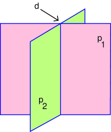
Figure 1: An orthogonal intersection of a $p_{1}$- and a $p_{2}$-brane along $d$ spatial directions.

Let us now add a probe $Dp_{2}$-brane sharing $d$ common spatial directions with the $p_{1}$-brane. The corresponding orthogonalintersection will be denoted as $(d|p_{1}\perp p_{2})$ and is depicted in Fig. 1. We will assume that the probe is extended along the directions $(x^{1},\ldots,x^{d},y^{1},\ldots,y^{p_{2}-d})$ and we will denote by $\vec{z}$ the set of $y$ coordinates transverse to the probe. Notice that $|\vec{z}|$ represents the separation of the branes along the directions transverse to both background and probe branes.

We will consider a static configuration in which the probe is located at a constant value of $|\vec{z}|$, namely at $|\vec{z}|=L$. The induced metric on the probe worldvolume for such a static configuration will be $ds^{2}_{I}={\cal G}_{ab}\,d\xi^{a}d\xi^{b}$ with $\xi^{a}$ being a set of worldvolume coordinates. In what follows we shall take these coordinates as the common Cartesian coordinates $x^{0},\ldots,x^{d}$, together with the spherical coordinates of the $y^{1},\ldots,y^{p_{2}-d}$ hyperplane. Assuming that $p_{2}-d\geq 2$, we will represent the line element of this hyperplane as

$$(dy^{1})^{2}+\cdots+(dy^{p_{2}-d})^{2}=d\rho^{2}+\rho^{2}\,d\Omega^{2}_{p_{2}-d-1}\,,$$ (27)

where $d\Omega^{2}_{p_{2}-d-1}$ is the line element of a unit $(p_{2}-d-1)$-sphere. It is now straightforward to verify that the induced metric $ds^{2}_{I}$ can be written as

$$ds^{2}_{I}=\biggl{[}{\rho^{2}+L^{2}\over R^{2}}\biggr{]}^{\alpha}dx^{2}_{1,d}+\biggl{[}{R^{2}\over\rho^{2}+L^{2}}\biggr{]}^{\alpha}(d\rho^{2}+\rho^{2}d\Omega^{2}_{p_{2}-d-1})\,.$$ (28)

Using Eqs. (25) and (28), we have that the energy for the probe-brane is

$$E=\biggl{[}{\rho^{2}+L^{2}\over R^{2}}\biggr{]}^{{\alpha\over 2}(d+1)-{\alpha\over 2}(p_{2}-d)-\gamma}\rho^{p_{2}-d-1}\sqrt{\det\tilde{g}}\,,$$ (29)

where $\tilde{g}$ is the metric of the unit $(p_{2}-d-1)$-sphere.

Since we are interested in studying BPS intersections, we have to impose that the branes do not exert any force among each other. This no-force condition requires the energy to be independent of the distance $L$ between the branes which, in view of the right-hand side of Eq. (29), is only possible if the number $d$ of common dimensions is related to the total dimensionality $p_{2}$ of the probe as

$$d={p_{2}\over 2}+{2\gamma-\alpha\over 2\alpha}\,.$$ (30)

Using (26), we get the following relation between $d$ and $p_{2}$:

$$d={p_{2}+p_{1}-4\over 2}\,.$$ (31)

However, as the brane of the background and the probe should live in the same theory, $p_{2}-p_{1}$ should be even. Since $d\leq p$, we are left with the following three possibilities $p_{2}=p_{1}$, $p_{1}+2$, $p_{1}+4$, for which Eq. (31) gives $d=p-2$, $p-1$, $p$ respectively. Thus, we get the following well-known set of orthogonal BPS intersections of $D$-branes:

$$(p\hskip 1.0pt|\hskip 1.0ptDp\perp D(p+4))\,,\qquad(p-1\hskip 1.0pt|\hskip 1.0ptDp\perp D(p+2))\,,\qquad(p-2\hskip 1.0pt|\hskip 1.0ptDp\perp Dp)\,.\ \$$ (32)

The cases of (32) give rise to three series of gauge/gravity dualities for gauge theories containing flavors confined to a defect; which in each case is of codimension 0, codimension 1 and codimension 2 in the ambient gauge theory. The gravity description is nothing but the $Dp_{1}$ background in which we embed the corresponding $Dp_{2}$ as probes, meanwhile for the first two series the field theory dual is the dimensional reduction of ${\mathcal{N}}=1$ $SU(N_{c})$ SYM in ten dimensions down to $d+1$ dimensions where we have to consider a 1/2 supersymmetric defect of the corresponding dimensionality containing fundamental matter with a global $SU(N_{f})$ symmetry. Given that the system is supersymmetric, it is possible to reconstruct the field theory in each case based on supersymmetry (and global symmetries) arguments. However, we will postpone a detailed field-theoretic analysis to Sec. 4 in order to give a more unified presentation of the different branches of the gauge theory.

The last intersection type deserves a particular comment, since it is somehow special. Given that both intersecting branes are of the same dimensionality, none of the local dynamics of the branes decouples from the system. Therefore, in the intersection, we have a product gauge group under which the matter is in the bifundamental representation, thus being not a flavoring of the “bulk” gauge theory in a proper sense.

3 The Coulomb Branch of the Gauge Theories

In the last section we argued that it is possible to find a gravity dual for defect field theories in terms of an intersection of branes in which the matter lives confined. In the brane-probe approximation, the gravity description corresponds to consider very few flavor branes suitably embedded in the near-horizon region of the background sourced by the (infinite) color branes, which partially overlap. On the other hand, the field theory dual corresponds to the gauge theory on the color branes plus the matter confined in the common intersection. As we anticipated, the color sector comes from the dimensional reduction down to the color brane worldvolume of the ${\cal{N}}=1$ ten-dimensional Yang–Mills theory. The matter comes from the open string sector connecting both brane stacks. Since both stacks will be separated a distance $L$, those strings will have a minimal length given by this $L$, so they will give rise to a massive matter sector with mass

$$m=\frac{L}{2\pi l_{s}^{2}}\,.$$ (33)

We have discussed the flavor probe branes with vanishing worldvolume vector field, which in particular had the consequence of not coupling the background RR potential to the probe worldvolume. Generically, a worldvolume vector field on a given brane has the effect of dissolving lower dimensional branes. This can be argumented through the Chern–Simons coupling

$$S_{\rm CS}=T_{p}\int P[e^{B}C^{(n)}]e^{2\pi l_{s}^{2}F}\,,$$ (34)

where it should be understood that a form of suitable dimensions should be constructed inside the integral. This way, one can couple $C^{(n)}$ to a $n+2$ brane through $F$ and to a $n+4$ brane through $F\wedge F$; meaning that both the $n+2$ and $n+4$ branes have $n$-brane charge dissolved. In the cases at hand, the RR potential will be that sourced by the color branes, so by turning on the worldvolume vector field we will be able to dissolve some of the color branes in the flavor ones. This way one would separate some of the branes of the color stack. But in the original picture, the stack of $N_{c}$ color branes gives rise to a $SU(N_{c})$ gauge theory, so separating the color branes amounts to break the gauge group down to some subgroup with a pattern given by the separation of the branes; which corresponds to a higgsing the gauge group. However, the separated branes are being dissolved in the flavor stack, which in turn requires to give some VEV’s to some of the open string fields. In particular, as we argued, we have to give a VEV to the worldvolume vector field. Since generically open string fields correspond to matter fields in the field theory, one would expect that, in addition to the breaking of the gauge group, some nontrivial quark VEV’s are generated, which should correspond to the Higgs branch of the theory.

On the other hand, taking the worldvolume gauge field to zero amounts to keep all the color branes agrupated in a single stack without recombining with the flavor ones. In particular, this means that we will not give any VEV to any open string field (matter sector in the field theory side), so this should correspond to the Coulomb phase of the gauge theory. Thus, the precise statement of the gauge/gravity duality is that the background of color branes with very few probe flavor branes with vanishing worldvolume gauge field corresponds to the Coulomb phase of the dual defect field theory.

3.1 Fluctuations as mesons

Since the probe branes we are considering in the background of the color ones have the interpretation of flavors in the field theory, their fluctuations will correspond to the possible excitations in the dual defect theory. In particular, if one finds a discrete spectrum for those fluctuations, this will correspond to the bound state spectrum of quarks (a.k.a. mesons) of the field theory. For the class of theories of interest, the meson spectrum study was initiated in [22] for the $D3-D7$ case, where the whole meson spectrum (in the Coulomb branch) was studied. However, a lot of work has been devoted towards studying the meson spectrum in various theories (in various contexts in several backgrounds; see for example [22, 23, 24, 25, 26, 27, 28, 29, 30, 31, 32, 33, 34, 35, 36, 37, 38, 39, 40, 41, 42, 43, 44, 45, 46, 47, 48, 49, 50, 51, 52, 53, 54]).

Let us study the fluctuations around the flavor brane embeddings discussed above. Without loss of generality we can take, for a generic $Dp_{1}-Dp_{2}$ intersection, $z^{1}=L$, $z^{m}=0$ ($m>1$) as the unperturbed configuration. Among all the fluctuations, we will restrict for simplicity to the transverse scalar modes $\chi$, which are of the type:

$$z^{1}=L+\chi^{1}\,,\qquad z^{m}=\chi^{m}(m>1)\,.$$ (35)

By analyzing the whole set of fluctuations, one can see that restricting to these modes is a consistent truncation (see [52] and [55]). The dynamics of the fluctuations is determined by the Dirac–Born–Infeld Lagrangian (23). By expanding this action and keeping up to second order terms, one can see that the relevant Lagrangian for the fluctuations is

$${\cal L}=-{1\over 2}\,\rho^{p_{2}-d-1}\sqrt{\det\tilde{g}}\biggl{[}{R^{2}\over\rho^{2}+L^{2}}\biggr{]}^{{7-p_{1}\over 4}}{\cal G}^{ab}\partial_{a}\chi^{m}\partial_{b}\chi^{m}\,,$$ (36)

where ${\cal G}^{ab}$ is the (inverse of the) metric (28). The equations of motion derived from ${\cal L}$ are

$$\partial_{a}\Bigg{[}{\rho^{p_{2}-d-1}\sqrt{\det\tilde{g}}\over(\rho^{2}+L^{2})^{{7-p_{1}\over 4}}}\,{\cal G}^{ab}\partial_{b}\chi\Bigg{]}=0\,,$$ (37)

where we have dropped the index $m$ in the $\chi$’s. Using the explicit form of the metric elements ${\cal G}^{ab}$, Eq. (37) can be written as the following differential equation:

$${R^{7-p_{1}}\over(\rho^{2}+L^{2})^{{7-p_{1}\over 2}}}\,\partial^{\mu}\partial_{\mu}\,\chi+{1\over\rho^{p_{2}-d-1}}\,\partial_{\rho}(\rho^{p_{2}-d-1}\partial_{\rho}\chi)+{1\over\rho^{2}}\,\nabla^{i}\nabla_{i}\chi=0\,,$$ (38)

where the index $\mu$ corresponds to the directions $x^{\mu}=(t,x^{1},\ldots,x^{d})$ and $\nabla_{i}$ is the covariant derivative on the $(p_{2}-d-1)$-sphere. To solve this equation, let us separate variables as

$$\chi=\xi(\rho)e^{ikx}Y^{l}(S^{p_{2}-d-1})\,,$$ (39)

where the product $kx$ is performed with the flat Minkowski metric and $Y^{l}(S^{p_{2}-d-1})$ are scalar spherical harmonics on the $(p_{2}-d-1)$-dimensional sphere, which satisfy

$$\nabla^{i}\nabla_{i}Y^{l}(S^{p_{2}-d-1})=-l(l+p_{2}-d-2)Y^{l}(S^{p_{2}-d-1})\,.$$ (40)

If we redefine the variables as

$$\varrho={\rho\over L}\,,\qquad\bar{M}^{2}=-R^{7-p_{1}}L^{p_{1}-5}k^{2}\,,$$ (41)

the differential equation (38) becomes

$$\partial_{\varrho}(\varrho^{p_{2}-d-1}\partial_{\varrho}\xi)+\bigg{[}\bar{M}^{2}\,{\varrho^{p_{2}-d-1}\over(1+\varrho^{2})^{{7-p_{1}\over 2}}}-l(l+p_{2}-d-2)\varrho^{p_{2}-d-3}\bigg{]}\xi=0\,.$$ (42)

For generic $p_{1}$, $p_{2}$, (42) has no simple analytic solution. However, a numerical analysis can be carried out. Generically, one obtains a discrete mass spectrum, being the masses of the mesons proportional to $L\sim m_{q}$. They will also depend on the inverse effective coupling, which is to be expected since the bound states should be a nonperturbative effect in the field theory. Remarkably, it turns out that in the $p_{1}=3$ case the differential equation (42) can be solved in terms of hypergeometric functions and the spectrum of values of $\bar{M}$ can be found exactly. Indeed, in this case, the fluctuations we have studied are a subset of those in [22]; where the whole spectrum was studied. We now turn to a more detailed analysis of this case.

3.1.1 $AdS_{5}\times S^{5}$ background

It is of particular interest the case of a bulk $(3+1)$-dimensional theory corresponding to a stack of color $D3$ branes. As we mentioned, this case was exhaustively studied in [22]. For $p_{1}=3$, in the limit we are considering in which the flavor branes are treated as probes, the decoupling limit works as in the usual $AdS/CFT$ case. Thus, once we take the decoupling limit, the gravity description is in terms of the corresponding embedding of the flavor branes in the near horizon of the $D3$ background, which is $AdS_{5}\times S^{5}$, being the possible flavorings

$$(3\hskip 1.0pt|\hskip 1.0ptD3\perp D7)\,,\qquad(2\hskip 1.0pt|\hskip 1.0ptD3\perp D5)\,,\qquad(1\hskip 1.0pt|\hskip 1.0ptD3\perp D3)\,.$$ (43)

Let us now introduce the quantity $\lambda$, related to the rescaled mass $\bar{M}$ as

$$\bar{M}^{2}=4\lambda(\lambda+1)\,.$$ (44)

Then, the solution of (42) for $p_{1}=3$ that is regular when $\varrho\to 0$ is

$$\xi(\varrho)=\varrho^{l}(\varrho^{2}+1)^{-\lambda}F\bigg{(}{-}\lambda,-\lambda+l-1+{p_{2}-d\over 2};l+{p_{2}-d\over 2};-\varrho^{2}\bigg{)}\,.$$ (45)

We also want that $\xi$ vanishes when $\varrho\to\infty$. A way to ensure this is by imposing that

$$-\lambda+l-1+{p_{2}-d\over 2}=-n\,,\quad n=0,1,2,\ldots\,.$$ (46)

When the quantization condition (46) is imposed, the series defining the hypergeometric function in (45) truncates, and the highest power of $\varrho$ is $(\varrho^{2})^{n}$. As a consequence $\xi$ vanishes as $\varrho^{-(l+p_{2}-d-2)}$ when $\varrho\to\infty$. Moreover, the quantization condition (46) of the values of $\lambda$ implies that the allowed values of $\bar{M}^{2}$ are

$$\bar{M}^{2}=4\bigg{(}n+l-1+{p_{2}-d\over 2}\bigg{)}\bigg{(}n+l+{p_{2}-d\over 2}\bigg{)}\,.$$ (47)

Notice that, for the three cases in (43), $p_{2}=2d+1$ for $d=3,2,1$. By using this relation between $p_{2}$ and $d$, one can rewrite the mass spectra (47) of scalar fluctuations for the intersections (43), corresponding to the meson spectrum in the Coulomb branch, as

$$M={2L\over R^{2}}\sqrt{\bigg{(}n+l+{d-1\over 2}\bigg{)}\bigg{(}n+l+{d+1\over 2}\bigg{)}}\,,$$ (48)

where $M^{2}=-k^{2}$ and we have taken into account that, in this case, $\bar{M}^{2}=-R^{4}L^{-2}k^{2}$ (see Eq. (41)).

It drops from (48) that the mass gap is proportional to $L$; which in turn is related to the quark mass. Indeed, in terms of field theory quantities we have that (48) reads

$$M={2\pi\over\sqrt{\lambda}}\,m_{q}\sqrt{2\bigg{(}n+l+{d-1\over 2}\bigg{)}\bigg{(}n+l+{d+1\over 2}\bigg{)}}\,,$$ (49)

so for zero quark mass the generated mass gap vanishes. Moreover, the induced metric on the probe (28) reduces to

$$ds^{2}_{I}={\rho^{2}+L^{2}\over R^{2}}\,dx_{1,d}^{2}+{R^{2}\over\rho^{2}+L^{2}}\,d\rho^{2}+R^{2}\,{\rho^{2}\over\rho^{2}+L^{2}}\,d\Omega^{2}_{d}\,.$$ (50)

In the so-called conformal case, corresponding to $L=0$, (50) reduces to $AdS_{d+2}\times S^{d}$, and therefore the dual theory is indeed a conformal field theory. Since a conformal theory does not generate a dynamical mass scale, and given that in the massless case there is no “tree-level” scale, the mass gap in the spectrum should vanish in the $L\sim m_{q}\rightarrow 0$ limit, as we found in (49). The defect conformal field theory is engineered as a defect which lives immersed in a ${\mathcal{N}}=4$ theory. This bulk theory enjoys a conformal symmetry, which naively one would expect to be broken by the addition of extra matter in the defect, even in the case in which the extra matter is massless. However, the conformal symmetry will appear just in the large $N_{c}$ and small $N_{f}$ limit, since there the would-be ADS (Affleck, Dine, Seiberg) superpotential vanishes.

In the massive case corresponding to $L\neq 0$, the bare mass of the quarks sets a scale which explicitly breaks the conformal symmetry. In turn, this is responsible for the appearance of the mass gap, since the meson masses are proportional to the scale $L$ corresponding to $m_{q}$. However, the same asymptotic $AdS$ metric is achieved in the ultraviolet limit $\rho\to\infty$. This $\varrho\to\infty$ limit is simply the high energy regime of the theory, where the mass of the quarks, which are proportional to the brane separation $L$, can be ignored and the theory becomes conformal. Therefore, one expects that the dual theory enjoys a conformal symmetry in the UV, and it is only in the IR, when the quark masses are relevant, that this conformal symmetry is broken and a mass gap with a discrete spectrum is generated.

The field theory lives in the boundary of the space, which corresponds to the large $\rho$ (namely UV) region. Since the UV regime is insensitive of the possible IR breaking of the conformal invariance, the $\varrho\to\infty$ behavior of the fluctuations, even in the $L\neq 0$ case, should provide us with information about the conformal dimension $\Delta$ of the corresponding operator. Taking into account that for large $\varrho$ the hypergeometric function behaves as

$$F(a_{1},a_{2};b;-\varrho^{2})\approx c_{1}\varrho^{-2a_{1}}+c_{2}\varrho^{-2a_{2}}\,,\quad(\varrho\to\infty)\,,$$ (51)

we have that $a_{1}=-\lambda$ and $a_{2}=-\lambda+l+{d-1\over 2}$. Using (8) in this case, we get the following value for the dimension of the operator associated to the scalar fluctuations:

$$\Delta=l+d\,.$$ (52)

It turns out that the mass spectra of all the Born–Infeld modes (and not only those reviewed here that correspond to the transverse scalars) can be computed analytically as in [22] (see also [52, 55] and [53]). This full set of fluctuation modes can be accommodated in multiplets, with the mass spectra displaying the expected degeneracy. The dual operators in the gauge theory side can be matched with the fluctuations by looking at the UV dimensions and at the R-charge quantum numbers. Generically, the dual fields are bilinear in the fundamental fields and contain the powers of the adjoint fields needed to construct the appropriate representation of the R-charge symmetry.

4 Higgsing the Theories

So far, in our gravity approximation to the systems we are interested in, we have not considered the effect of the RR gauge field in the worldvolume of the probe flavor branes. As we argued, the reason is that we considered a vanishing worldvolume gauge field on the probe branes. In turn, this field is required in order to couple such RR background potential to the worldvolume theory. However, as we argued, we have reasons to believe that the inclusion of this field will correspond to the Higgs branch of the theory. As we already described, the reason is that, by means of this field, we can dissolve some of the color branes in the flavor ones. Heuristically, as already suggested in [67], this would represent separating some of the color branes and therefore breaking the gauge group. But moreover, those color branes are being dissolved in the flavor ones, which gives some VEV’s to some open string fields, which in turn should correspond to quark VEV’s. Thus, on very general grounds, one would expect that the dual field theory is in the Higgs branch. In this section we will explicitly see how it is the case. Actually, by considering as examples the flavorings of ${\mathcal{N}}=4$, we will explicitly discuss the field theories and explore how they contain different branches apart from the Coulomb phase already discussed.

4.1 The codimension zero defect

We will first study the codimension 0 intersection. This corresponds to the $Dp-Dp+4$ intersection where the flavors fill the whole bulk where the gauge theory lives:

$$\begin{array}[]{rccccccccccl}&1&\cdots&p&p+1&p+2&p+3&p+4&p+5&\cdots&9&\\[2.0pt] Dp:&\times&\cdots&\times&-&-&-&-&-&\cdots&-&\\[2.0pt] D(p+4):&\times&\cdots&\times&\times&\times&\times&\times&-&\cdots&-&\end{array}$$

From the gravity side, all the cases behave in a similar way. However, we will examine the $p=3$ case, where a detailed description of both the field theory and gravity side will be given. The other cases will behave in a similar way, and indeed, when computing the fluctuations giving rise to the mesons, we will treat in a unified way all the dimensionalities.

4.1.1 A case study I$:$ the $D3-D7$ intersection

Let us start considering the $D3-D7$ intersection first studied in [63] and further analyzed in [65]. It can be seen that the dual gauge theory is a ${\mathcal{N}}=2$ SYM theory in $3+1$ dimensions obtained by adding $N_{f}$ ${\mathcal{N}}=2$ fundamental hypermultiplets to the ${\mathcal{N}}=4$ $SYM$ theory, in which, as we know, the transverse separation of the branes gives a bare mass to the quarks. The Lagrangian is given by [63]

$${\cal L} = \tau\int d^{\hskip 0.5pt2}\theta\,d^{\hskip 0.5pt2}\bar{\theta}\big{(}Tr\big{(}\Phi_{I}^{\dagger}e^{V}\Phi_{I}e^{-V}\big{)}+Q_{i}^{\dagger}e^{V}Q^{i}+\tilde{Q}_{i}e^{-V}\tilde{Q}^{i\dagger}\big{)}$$ (54)

$${}+\tau\int d^{\hskip 0.5pt2}\theta(Tr({\cal W}^{\alpha}{\cal W}_{\alpha})+W)+\tau\int d^{\hskip 0.5pt2}\bar{\theta}(Tr(\bar{\cal W}_{\dot{\alpha}}\bar{\cal W}^{\dot{\alpha}})+\bar{W})\,,$$

where the superpotential is

$$W=\tilde{Q}_{i}(m+\Phi_{3})Q^{i}+{1\over 3}\,\epsilon^{IJK}Tr[\Phi_{I}\Phi_{J}\Phi_{K}]\,.$$ (55)

In Eq. (54) we are working in ${\cal N}=1$ language, where $Q_{i}$, ($\tilde{Q}_{i}$) $i=1,\ldots,N_{f}$ are the chiral (antichiral) superfields in the hypermultiplet, while $\Phi_{I}$ are the adjoint scalars of ${\mathcal{N}}=4$ SYM once complexified as $\Phi_{1}=X^{1}+iX^{2}$, $\Phi_{2}=X^{3}+iX^{4}$ and $\Phi_{3}=X^{5}+iX^{6}$; where $X^{I}$ ($I=1,\ldots,6$) is the scalar which corresponds to the direction $I+3$ in the array (4.1). It is worth mentioning that an identity matrix in color space is to be understood to multiply the mass parameter of the quarks $m$.

We are interested in the classical SUSY vacua of this theory, which can be obtained by imposing the corresponding $D$- and $F$-flatness conditions following from the Lagrangian (54). The vanishing of the $F$-terms corresponding to the quark hypermultiplets amounts to set:

$$\tilde{Q}_{i}(\Phi_{3}+m)=0\,,\quad(\Phi_{3}+m)Q^{i}=0\,.$$ (56)

In turn, the vanishing of the $F$-terms associated to the adjoint scalars gives rise to

$$[\Phi_{1},\Phi_{3}]=[\Phi_{2},\Phi_{3}]=0\,,$$ (57)

together with the equation

$$Q^{i}\tilde{Q}_{i}+[\Phi_{1},\Phi_{2}]=0\,.$$ (58)

In (58) $Q^{i}\tilde{Q}_{i}$ denotes a matrix in color space of components $Q^{i}_{\alpha}\tilde{Q}_{i}^{\beta}$.

In addition to the $F$-flatness condition, we also have to impose the $D$-flatness

$$|Q^{i}|^{2}-|\tilde{Q}_{i}|^{2}+[\Phi_{1},\Phi_{1}^{\dagger}]+[\Phi_{2},\Phi_{2}^{\dagger}]=0\,.$$ (59)

Note that $|Q^{i}|^{2}=Q^{i}_{\alpha}(Q^{i}_{\beta})^{\dagger}$ is also a matrix in color space, as well as the commutator of the $\Phi$ fields, since they are in the adjoint representation of the $SU(N)$ gauge group.

Let us start considering the Coulomb branch of the theory, which corresponds to setting all the $Q$, $\tilde{Q}$ are zero. This forces to take the $\Phi_{i}$ as commuting matrices. In general, they will be of the form

$$\Phi_{i}=\left(\begin{array}[]{c c c c c}m_{i}^{1}&0&\cdots&0&0\\ 0&m_{i}^{2}&\cdots&0&0\\ \vdots&\vdots&\ddots&\vdots&\vdots\\ 0&0&\cdots&m_{i}^{N_{c}-1}&0\\ 0&0&\cdots&0&m_{i}^{N_{c}}\end{array}\right)\ .$$

begin the $m_{i}^{\alpha}$ some constants. Motion along the Coulomb branch amounts to consider different $m_{i}^{\alpha}$. Since the eigenvalues of the adjoint fields have the interpretation of the transverse coordinates to the color branes, changing the $m_{i}^{\alpha}$ represents slight separations of the background $D3$; so moving along the Coulomb branch amounts to changing the different relative positions of each color brane. Actually, this implies that in a generic point of the Coulomb branch we will have a broken gauge group according to the particular brane separation pattern.

However, as shown in [65], from (56) it is clear that whenever some eigenvalues of the $\Phi_{3}$ matrix are set to $-m$ we have the possibility of developing a nonzero value for the $Q$, $\tilde{Q}$ in the corresponding entry of the matrix while still satisfying the $F$-term flatness condition. Since we are giving a VEV to some quark fields, we are entering the Higgs branch of the theory. Indeed, in order to give this nonzero VEV’s, we had to choose in a given way the $\Phi_{3}$ eigenvalues, breaking the gauge group down to some subgroup by moving in the Coulomb branch. Therefore, as it is well-known, we see that we must to go to a particular point of the Coulomb branch (namely that with some entries of $\Phi_{3}$ set to $-m$) to have the possibility to develop a nonzero VEV for the quarks and enter Higgs branch (see for example [66] for an argumentation of this in a different context which we will shortly review below). In general, we can go to the Higgs branch considering a solution to (56) as

$$\Phi_{3}=\left(\begin{array}[]{@{\hspace{1pt}}cccccc@{\hspace{1pt}}}\hskip 1.0pt\lx@intercol\hfil\tilde{m}_{1}&&&&&\hfil\hskip 1.0\\ \hskip 1.0pt\lx@intercol\hfil&\ddots&&&\\ \hskip 1.0pt\lx@intercol\hfil&&\tilde{m}_{N-k}&&&\hfil\hskip 1.0\\ \hskip 1.0pt\lx@intercol\hfil&&&-m&&\hfil\hskip 1.0\\ \hskip 1.0pt\lx@intercol\hfil&&&&\ddots&\hfil\hskip 1.0\\ \hskip 1.0pt\lx@intercol\hfil&&&&&-m\hfil\hskip 1.0\end{array}\right)\,,$$ (66)

where the number of $m$’s is $k$. In order to have $\Phi_{3}$ in the Lie algebra of $SU(N)$, one must have $\sum_{j=1}^{N-k}\tilde{m}_{j}=km$. This choice of $\Phi_{3}$ lead us to take $Q^{i}$ and $\tilde{Q}_{i}$ as

$$\tilde{Q}_{i}=(0\cdots 0,\tilde{q}^{1}_{i},\ldots,\tilde{q}^{k}_{i})\,,\qquad Q^{i}=\left(\begin{array}[]{c}0\\ \vdots\\ 0\\ q^{i}_{1}\\ \vdots\\ q^{i}_{k}\end{array}\right)\,.$$ (73)

Indeed, it is trivial to check that the values of $\Phi_{3}$, $\tilde{Q}_{i}$ and $Q^{i}$ displayed in Eqs. (66) and (73) solve Eq. (56). Since the quark VEV in this solution has some components which are zero and others that are different from zero, this choice of vacuum leads to a so-called mixed Coulomb–Higgs phase.

For a vacuum election as in Eq. (73) we can restrict ourselves to the lower $k\times k$ matrix block, and we can write Eq. (58) as

$$q^{i}\tilde{q}_{i}+[\Phi_{1},\Phi_{2}]=0\,,$$ (74)

where now, and it what follows, it is understood that $\Phi_{1}$ and $\Phi_{2}$ are $k\times k$ matrices. In addition, we can write the $D$-term restricted to just this $k\times k$ subspace inside the color space as

$$|q^{i}|^{2}-|\tilde{q}_{i}|^{2}+[\Phi_{1},\Phi_{1}^{\dagger}]+[\Phi_{2},\Phi_{2}^{\dagger}]=0\,.$$ (75)

The constraints (74) and (75), together with the condition $[\Phi^{I},\Phi^{3}]=0$, define the mixed Coulomb–Higgs phase of the theory.

Gravity dual of the mixed Coulomb–Higgs phase

An important point coming from the field theory discussion is that in order to enter the Higgs branch of the theory we need to go to a particular point in the Coulomb branch. Given that the eigenvalues of the adjoint fields represent the positions of the individual branes of the color stack, this particular point on the Coulomb branch allowing for the Higgs branch should correspond to having some of the color branes away from the others and coincident in the $(8,9)$ directions, which the $\Phi_{3}$ field represent. This branes precisely sit at a distance $m$ to the origin, where the flavor $D7$ sits in the brane construction. It is then natural to guess that these $D3$ are dissolved as instantons in the flavor $D7$, with the quark VEV’s being the responsibles of the dissolution. Since as we argued dissolving lower-dimensional branes is done via a nontrivial configuration of the worldvolume gauge field, on the worldvolume of the flavor $D7$ there should be an instantonic magnetic field. Indeed, as it is well-known, there is a one-to-one correspondence between the Higgs phase of ${\cal{N}}=2$ gauge theories and the moduli space of instantons [84, 85, 86]. This comes from the fact that the $F$- and $D$-flatness conditions can be directly mapped into the ADHM equations (see [87] and [88] for reviews). Because of this map, we can identify the Higgs phase of the gauge theory with the space of four-dimensional instantons; which, in the context at hand, can be understood in terms of the instantonic worldvolume vector field necessary to dissolve $D3$ inside the $D7$. Actually, this provides a natural interpretation of the Higgs phase-ADHM equations map.

To summarize, the gravity dual of the Higgs phase of the field theory above is realized in terms of a $D7$ brane with dissolved $D3$ representing the separation and further dissolution of some of the color branes in the flavor ones. Therefore, once we take the decoupling limit, the gravity dual of the field theory in the previous subsection corresponds to the near-horizon of the color branes where we should embed the flavor ones as probes. In the case at hand, the corresponding background is $AdS_{5}\times S^{5}$, which also includes a 4-form RR potential given by

$$C^{(4)}=\bigg{(}\frac{r^{2}}{R^{2}}\bigg{)}^{2}\ dx^{0}\wedge\cdots\wedge dx^{3}\,.$$ (76)

Then, in order to couple (76) to the worldvolume of the flavor brane, we see that indeed we have to include the instantonic worldvolume gauge field along the coordinates in the $D7$ transverse to the $D3$. Let us concrete, and write the $AdS_{5}\times S^{5}$ background in a system of coordinates suitable for our purposes. Let $\vec{y}=(y^{1},\ldots,y^{4})$ be the coordinates along the directions $4,\ldots,7$ in the array (4.1) and let us denote by $\rho$ the length of $\vec{y}$ (i.e. $\rho^{2}=\vec{y}\cdot\vec{y}$). Moreover, we will call $\vec{z}=(z^{1},z^{2})$ the coordinates $8,9$ of (4.1). Notice that $\vec{z}$ is a vector in the directions which are orthogonal to both stacks of D-branes. Clearly, $r^{2}=\rho^{2}+\vec{z}^{2}$, so the metric can be written as

$$ds^{2}=\frac{\rho^{2}+\vec{z}^{2}}{R^{2}}\,dx^{2}_{1,3}+\frac{R^{2}}{\rho^{2}+\vec{z}^{2}}\,(d\vec{y}^{2}+d\vec{z}^{2})\,.$$ (77)

The DBI action for a stack of $N_{f}$ $D7$-branes with worldvolume gauge field is given by

$$S_{\rm DBI}^{D7}=-T_{7}\int d^{8}\xi\,e^{-\phi}Str\big{\{}\sqrt{-\det(g+F)}\big{\}}\,,$$ (78)

where $\xi^{a}$ is a system of worldvolume coordinates, $\phi$ is the dilaton, $g$ is the induced metric and $F$ is the field strength of the $SU(N_{f})$ worldvolume gauge group. Let us assume that we take $\xi^{a}=(x^{\mu},y^{i})$ as worldvolume coordinates and that we consider a $D7$-brane embedding in which $|\vec{z}|=L$, where $L$ represents the constant transverse separation between the two stacks of $D3$- and $D7$-branes. Notice that this transverse separation will give a mass $L/2\pi\alpha^{\prime}$ to the $D3-D7$ strings, which corresponds to the quark mass in the field theory dual. For an embedding with $|\hskip 0.5pt\vec{z}\hskip 0.5pt|=L$, the induced metric takes the form

$$g_{x^{\mu}x^{\nu}}={\rho^{2}+L^{2}\over R^{2}}\,\eta_{\mu\nu}\,,\qquad g_{y^{i}y^{j}}={R^{2}\over\rho^{2}+L^{2}}\,\delta_{ij}\,.$$ (79)

Let us now assume that the worldvolume field strength $F$ has nonzero entries only along the directions of the $y^{i}$ coordinates and let us denote $F_{y^{i}y^{j}}$ simply by $F_{ij}$. Then, after using Eq. (79) and the fact that the dilaton is trivial for the$AdS_{5}\times S^{5}$ background, the DBI action (78) takes the form

$$S_{\rm DBI}^{D7}=-T_{7}\int d^{\hskip 0.5pt4}x\,d^{\hskip 0.5pt4}yStr\Bigg{\{}\sqrt{\det\bigg{(}\delta_{ij}+\bigg{(}\frac{\rho^{2}+L^{2}}{R^{2}}\bigg{)}F_{ij}\bigg{)}}\,\Bigg{\}}\,.$$ (80)

The matrix appearing on the r.h.s. of Eq. (80) is a $4\times 4$ matrix whose entries are $SU(N_{f})$ matrices. However, inside the symmetrized trace such matrices can be considered as commutative numbers. Actually, we will evaluate the determinant in (80) by means of the following identity. Let $M_{ij}=-M_{ji}$ be a $4\times 4$ antisymmetric matrix. Then, one can check that

$$\det(1+M)=1+{1\over 2}\,M^{2}+{1\over 16}\,({}^{*}MM)^{2}\,,$$ (81)

where $M^{2}$ and ${}^{*}MM$ are defined as follows:

$$M^{2}\equiv M_{ij}M_{ij}\,,\qquad{}^{*}MM\equiv{}^{*}M_{ij}M_{ij}\,,$$ (82)

and ${}^{*}M$ is defined as the following matrix:

$${}^{*}M_{ij}={1\over 2}\,\epsilon_{ijkl}M_{kl}\,.$$ (83)

When the $M_{ij}$ matrix is self-dual (i.e. when ${}^{*}M=M$), the three terms on the r.h.s. of (81) build up a perfect square:

$$\det(1+M)|_{self-dual}=\bigg{(}1+{1\over 4}\,M^{2}\bigg{)}^{2}\,.$$ (84)

Let us consider a configuration in which the worldvolume gauge field is self-dual in the internal $R^{4}$ of the worldvolume spanned by the $y^{i}$ coordinates which, as one can check, satisfies the equations of motion of the $D7$-brane probe. For such an instantonic gauge configuration ${}^{*}F=F$, where ${}^{*}F$ is defined following Eq. (83). Using the expression in Eq. (84), we can write

$$S_{\rm DBI}^{D7}\hbox{(self-dual)}=-T_{7}\int d^{\hskip 0.5pt4}x\,d^{\hskip 0.5pt4}yStr\bigg{\{}1+\frac{1}{4}\bigg{(}\frac{\rho^{2}+L^{2}}{R^{2}}\bigg{)}^{2}{}^{*}FF\bigg{\}}\,.$$ (85)

In turn, the WZ piece of the worldvolume action reduces in this case to

$$S_{\rm WZ}^{D7}={T_{7}\over 2}\int Str\big{[}P\big{[}C^{(4)}\big{]}\wedge F\wedge F\big{]}\,,$$ (86)

By using the same set of coordinates as in (80), and the explicit expression of $C^{(4)}$ (see Eq. (76)), one can rewrite $S_{\rm WZ}^{D7}$ as

$$S_{\rm WZ}^{D7}=T_{7}\int d^{\hskip 0.5pt4}x\,d^{\hskip 0.5pt4}yStr\bigg{\{}\frac{1}{4}\bigg{(}\frac{\rho^{2}+L^{2}}{R^{2}}\bigg{)}^{2}{}^{*}FF\bigg{\}}\,.$$ (87)

Remarkably, once we assume the instantonic character of $F$, the WZ term partially cancels the DBI giving

$$S^{D7}\hbox{(self-dual)}=-T_{7}\int d^{\hskip 0.5pt4}x\,d^{\hskip 0.5pt4}yStr[1]=-T_{7}N_{f}\int d^{\hskip 0.5pt4}x\,d^{\hskip 0.5pt4}y\,.$$ (88)

Notice that in the total action (88) the transverse distance $L$ does not appear. This “no-force” condition is an explicit manifestation of the SUSY of the system. Indeed, the fact that the DBI action is a square root of a perfect square is required for supersymmetry, and actually can be regarded as the saturation of a BPS bound. Furthermore, had we changed the sign of the WZ by considering an antibrane rather than a brane, we would have had an explicit appearance of $L$, breaking the no-force condition since the system would be nonsupersymmetric.

In order to get a proper interpretation of the role of the instantonic gauge field on the $D7$-brane probe, let us recall that for self-dual configurations the integral of the Pontryagin density ${\cal P}(y)$ is quantized for topological reasons. Actually, with our present normalization of $F$, ${\cal P}(y)$ is given by

$${\cal P}(y)\equiv\frac{1}{16\pi^{2}}\,{1\over(2\pi\alpha^{\prime})^{2}}Tr[{}^{*}FF]\,,$$ (89)

and, if $k\in Z$ is the instanton number, one has

$$\int d^{\hskip 0.5pt4}y\,{\cal P}(y)=k\,.$$ (90)

A worldvolume gauge field satisfying (90) is inducing $k$ units of $D3$-brane charge into the $D7$-brane worldvolume along the subspace spanned by the Minkowski coordinates $x^{\mu}$. To verify this fact, let us rewrite the WZ action (86) of the $D7$-brane as

$$S_{\rm WZ}^{D7}={T_{7}\over 4}\int d^{\hskip 0.5pt4}x\,d^{\hskip 0.5pt4}y\,C_{x^{0}x^{1}x^{2}x^{3}}^{(4)}Tr[{}^{*}FF]=T_{3}\int d^{\hskip 0.5pt4}x\,d^{\hskip 0.5pt4}y\,C_{x^{0}x^{1}x^{2}x^{3}}^{(4)}{\cal P}(y)\,,$$ (91)

where we have used (89) and the relation $T_{3}=(2\pi)^{4}\,(\alpha^{\prime})^{2}\,T_{7}$ between the tensions of the $D3$- and $D7$-branes. If $C_{x^{0}x^{1}x^{2}x^{3}}^{(4)}$ does not depend on the coordinate $y$, we can integrate over $y$ by using Eq. (90), namely

$$S_{\rm WZ}^{D7}=kT_{3}\int d^{\hskip 0.5pt4}x\,C_{x^{0}x^{1}x^{2}x^{3}}^{(4)}\,.$$ (92)

Equation (92) shows that the coupling of the $D7$-brane with $k$ instantons in the worldvolume to the RR potential $C^{(4)}$ of the background is identical to the one corresponding to $k$ $D3$-branes, as claimed above. It is worth to remark here that the existence of these instanton configurations relies on the fact that we are considering $N_{f}>1$ flavor $D7$ branes, i.e. that we have a non-Abelian worldvolume gauge theory.

Recovering the field theory picture from the microscopical interpretation of the $D3-D7$ intersection with flux

The fact that the $D7$-branes carry $k$ dissolved $D3$-branes on them opens up the possibility of a new perspective on the system, which could be regarded not just from the point of view of the $D7$-branes with dissolved $D3$s, but also from the point of view of the dissolved $D3$-branes which expand due to dielectric effect [68] to a transverse fuzzy $R^{4}$ (see the appendix for a very short introduction to the dielectric effect). From this point of view, the $D7$ appears as an effective description, which we will call “macroscopic,” while the picture in terms of blown-up $D3$ will be called “microscopic.” Going back to the field theory description, the fact that, once we are in the adequate point in the Coulomb branch, we enter the fields $\Phi_{1},\Phi_{2}$ are matrix-valued suggest precisely that we can think those $D3$ at $m$ distance to expand dielectrically to an effective $D7$ brane. To see this, let us assume that we have a stack of $k$ $D3$-branes in the background given by (77). These $D3$-branes are extended along the four Minkowski coordinates $x^{\mu}$, whereas the transverse coordinates $\vec{y}$ and $\vec{z}$ must be regarded as the matrix scalar fields $Y^{i}$ and $Z^{j}$, taking values in the adjoint representation of $SU(k)$. Actually, we will assume in what follows that the $Z^{j}$ scalars are Abelian, as it corresponds to a configuration in which the $D3$-branes are localized (i.e. not polarized) in the space transverse to the $D7$-brane.

The dynamics of a stack of coincident $D3$-branes is determined by the Myers dielectric action [68] (see Appendix), which is the sum of a Dirac–Born–Infeld and a Wess–Zumino part:

$$S_{D3}=S_{\rm DBI}^{D3}+S_{\rm WZ}^{D3}\,.$$ (93)

For the background we are considering the DBI action is

$$S_{\rm DBI}^{D3}=-T_{3}\int d^{\hskip 0.5pt4}\xi Str\Big{[}\sqrt{-\det[P[G+G(Q^{-1}-\delta)G]_{ab}]}\sqrt{\det Q}\,\Big{]}\,,$$ (94)

In Eq. (94) $G$ is the background metric, ${\bf Str}(\cdots)$ represents the symmetrized trace over the $SU(k)$ indices and $Q$ is a matrix which depends on the commutator of the transverse scalars (see below). The WZ term for the $D3$-brane in the $AdS_{5}\times S^{5}$ background under consideration is

$$S_{\rm WZ}^{D3}=T_{3}\int d^{\hskip 0.5pt4}\xi Str\big{[}P\big{[}C^{(4)}\big{]}\big{]}\,.$$ (95)

As we are assuming that only the $Y$ scalars are noncommutative, the only elements of the matrix $Q$ appearing in (94) that differ from those of the unit matrix are given by

$$Q_{y^{i}y^{j}}=\delta_{ij}+{i\over 2\pi\alpha^{\prime}}[Y^{i},Y^{k}]G_{y^{k}y^{j}}\,.$$ (96)

By using the explicit form of the metric elements along the $y$ coordinates (see Eq. (77)), one can rewrite $Q_{ij}$ as

$$Q_{y^{i}y^{j}}=\delta_{ij}+{i\over 2\pi\alpha^{\prime}}\,{R^{2}\over\hat{r}^{2}}\,[Y^{i},Y^{j}]\,,$$ (97)

where $\hat{r}^{\,2}$ is the matrix

$$\hat{r}^{2}=(Y^{i})^{2}+Z^{2}\,.$$ (98)

Let us now define the matrix $\theta_{ij}$ as

$$i\theta_{ij}\equiv{1\over 2\pi\alpha^{\prime}}\,[Y^{i},Y^{j}]\,.$$ (99)

It follows from this definition that $\theta_{ij}$ is antisymmetric in the $i,j$ indices and, as an $SU(k)$ matrix, is Hermitian:

$$\theta_{ij}=-\theta_{ji}\,,\qquad\theta_{ij}^{\dagger}=\theta_{ij}\,.$$ (100)

The algebra given by (99) defines a fuzzy $R^{4}$ (see for example [89]). The appearance of this algebra should be expected, since from the macroscopical picture we expect the $D3$ to polarize into a transverse $R^{4}$ giving rise to the effective $D7$.

Moreover, in terms of $\theta_{ij}$, the matrix $Q_{ij}$ can be written as

$$Q_{y^{i}y^{j}}=\delta_{ij}-{R^{2}\over\hat{r}^{2}}\theta_{ij}\,.$$ (101)

Using these definitions, we can write the DBI action (94) for the dielectric $D3$-brane in the $AdS_{5}\times S^{5}$ background as

$$S_{\rm DBI}^{D3}=-T_{3}\int d^{\hskip 0.5pt4}x\ \,{\bf Str}\Bigg{[}\bigg{(}{\hat{r}^{2}\over R^{2}}\bigg{)}^{2}\sqrt{\det\bigg{(}\delta_{ij}-{R^{2}\over\hat{r}^{2}}\theta_{ij}\bigg{)}}\,\Bigg{]}\,,$$ (102)

where we have chosen the Minkowski coordinates $x^{\mu}$ as our set of worldvolume coordinates for the dielectric $D3$-brane. Similarly, the WZ term can be written as

$$S_{\rm WZ}^{D3}=T_{3}\int d^{\hskip 0.5pt4}x\ \,{\bf Str}\bigg{[}\bigg{(}{\hat{r}^{2}\over R^{2}}\bigg{)}^{2}\bigg{]}\,.$$ (103)

Let us now assume that the matrices $\theta_{ij}$ are self-dual with respect to the $ij$ indices, i.e. that ${}^{*}\theta=\theta$. Notice that, in terms of the original matrices $Y^{i}$, this is equivalent to the condition

$$[Y^{i},Y^{j}]=\frac{1}{2}\epsilon_{ijkl}[Y^{k},Y^{l}]\,.$$ (104)

Moreover, the self-duality condition implies that there are three independent $\theta_{ij}$ matrices, namely

$$\theta_{12}=\theta_{34}\,,\qquad\theta_{13}=\theta_{42}\,,\qquad\theta_{14}=\theta_{23}\,.$$ (105)

The description of the $D3-D7$ system from the perspective of the color $D3$-branes should match the field theory analysis performed at the beginning of this section. In particular, the $D$- and $F$-flatness conditions of the adjoint fields in the Coulomb–Higgs phase of the ${\cal N}=2$ SYM with flavor should be the same as the ones satisfied by the transverse scalars of the dielectric $D3$-brane. Let us define the following complex combinations of the $Y^{i}$ matrices:

$$2\pi\alpha^{\prime}\Phi_{1}\equiv{Y^{1}+iY^{2}\over\sqrt{2}}\,,\qquad 2\pi\alpha^{\prime}\Phi_{2}\equiv{Y^{3}+iY^{4}\over\sqrt{2}}\,,$$ (106)

where we have introduced the factor $2\pi\alpha^{\prime}$ to take into account the standard relation between coordinates and scalar fields in string theory. We are going to identify $\Phi_{1}$ and $\Phi_{2}$ with the adjoint scalars of the field theory side. From the definitions (99) and (106) and the self-duality condition (105), it is straightforward tocheck that

$$[\,\Phi_{1}\,,\Phi_{2}\,]\,=\,-{\theta_{23}\over 2\pi\alpha^{\prime}}\,+\,i{\theta_{13}\over 2\pi\alpha^{\prime}}\,\,,$$ (107)

$$[\,\Phi_{1}\,,\Phi_{1}^{\dagger}\,]\,=\,[\,\Phi_{2}\,,\Phi_{2}^{\dagger}\,]\,=\,{\theta_{12}\over 2\pi\alpha^{\prime}}\,\,.$$ (108)

By comparing with the results of the field theory analysis (Eqs. (74) and (59)), we get the following identifications between the $\theta$’s and the vacuum expectation values of the matter fields:

$$q^{i}\tilde{q}_{i}={\theta_{23}\over 2\pi\alpha^{\prime}}-i{\theta_{13}\over 2\pi\alpha^{\prime}}\,,\qquad|\tilde{q}_{i}|^{2}-|q^{i}|^{2}={\theta_{12}\over\pi\alpha^{\prime}}\,.$$ (109)

Moreover, from the point of view of this dielectric description, the $\Phi_{3}$ field in the field theory is proportional to $Z^{1}+iZ^{2}$. Since the stack of branes is localized in that directions, $Z^{1}$ and $Z^{2}$ are Abelian and clearly we have that $[\Phi_{1},\Phi_{3}]=[\Phi_{2},\Phi_{3}]=0$, thus matching the last $F$-flatness condition for the adjoint field $\Phi_{3}$.

It is also interesting to relate the present microscopic description of the $D3-D7$ intersection, in terms of a stack of dielectric $D3$-branes, to the macroscopic description, in terms of the flavor $D7$-branes. With this purpose in mind, let us compare the actions of the $D3$- and $D7$-branes. First of all, we notice that, when the matrix $\theta$ is self-dual, we can use Eq. (84) and write the DBI action (102) as

$$S_{\rm DBI}^{D3}\hbox{(self-dual)}=-T_{3}\int d^{\hskip 0.5pt4}x\ \,{\bf Str}\bigg{[}\bigg{(}{\hat{r}^{2}\over R^{2}}\bigg{)}^{2}+{1\over 4}\,\theta^{2}\bigg{]}\,.$$ (110)

Moreover, by inspecting Eqs. (103) and (110) we discover that the WZ action cancels against the first term of the right-hand side of (110), in complete analogy to what happens to the $D7$-brane. Thus, one has

$$S^{D3}\hbox{(self-dual)}=-{T_{3}\over 4}\int d^{\hskip 0.5pt4}x\,{\bf Str}[\theta^{2}]=-\pi^{2}T_{7}(2\pi\alpha^{\prime})^{2}\int d^{\hskip 0.5pt4}x\,{\bf Str}[\theta^{2}]\,,$$ (111)

where, in the last step, we have rewritten the result in terms of the tension of the $D7$-brane. Moreover, an important piece of information is obtained by comparing the WZ terms of the $D7$- and $D3$-branes (Eqs. (91) and (103)). Actually, from this comparison we can establish a map between matrices in the $D3$-brane description and functions of the $y$ coordinates in the $D7$-brane approach. Indeed, let us suppose that $\hat{f}$ is a $k\times k$ matrix and let us call $f(y)$ the function to which $\hat{f}$ is mapped. It follows from the identification between the $D3$- and $D7$-brane WZ actions that the mapping rule is

$$\,{\bf Str}[\hat{f}]\Rightarrow\int d^{\hskip 0.5pt4}y\,{\cal P}(y)f(y)\,,$$ (112)

where the kernel ${\cal P}(y)$ on the r.h.s. of (112) is the Pontryagin density defined in Eq. (89). Actually, the comparison between both WZ actions tells us that the matrix $\hat{r}^{2}$ is mapped to the function $\vec{y}^{\,2}+\vec{z}^{\,2}$. Notice also that, when $\hat{f}$ is the unit $k\times k$ matrix and $f(y)=1$, both sides of (112) are equal to the instanton number $k$ (see Eq. (90)). Another interesting information comes by comparing the complete actions of the $D3$- and $D7$-branes. It is clear from (111) and (88) that

$$(2\pi\alpha^{\prime})^{2}\,{\bf Str}[\theta^{2}]\Rightarrow\int d^{\hskip 0.5pt4}y\,{N_{f}\over\pi^{2}}\,.$$ (113)

By comparing Eq. (113) with the general relation (112), one gets the function that corresponds to the matrix $\theta^{2}$, namely

$$(2\pi\alpha^{\prime})^{2}\theta^{2}\Rightarrow{N_{f}\over\pi^{2}{\cal P}(y)}\,.$$ (114)

Notice that $\theta^{2}$ is a measure of the noncommutativity of the adjoint scalars in the dielectric approach, i.e. is a quantity that characterizes the fuzziness of the space transverse to the $D3$-branes. Equation (114) is telling us that this fuzziness is related to the (inverse of the) Pontryagin density for the macroscopic $D7$-branes. Actually, this identification is reminiscent of the one found in [90] between the noncommutative parameter and the NSNS $B$-field in the string theory realization of noncommutative geometry. Interestingly, in our case the commutator matrix $\theta$ is related to the VEV of the matter fields $q$ and $\tilde{q}$ through the $F$- and $D$-flatness conditions (74) and (59). Notice that Eq. (114) implies that the quark VEV is somehow related to the instanton density on the flavor brane. In order to make this correspondence more precise, let us consider the one-instanton configuration of the $N_{f}=2$ gauge theory on the $D7$-brane worldvolume. In the so-called singular gauge, the $SU(2)$ gauge field is given by

$${A_{i}\over 2\pi\alpha^{\prime}}=2i\Lambda^{2}\frac{\bar{\sigma}_{ij}y^{j}}{\rho^{2}(\rho^{2}+\Lambda^{2})}\,,$$ (115)

where $\rho^{2}=\vec{y}\cdot\vec{y}$, $\Lambda$ is a constant (the instanton size) and the matrices $\bar{\sigma}_{ij}$ are defined as

$$\bar{\sigma}_{ij}={1\over 4}\,(\bar{\sigma}_{i}\sigma_{j}-\bar{\sigma}_{j}\sigma_{i})\,,\quad\sigma_{i}=(i\vec{\tau},1_{2\times 2})\,,\quad\bar{\sigma}_{i}=\sigma_{i}^{\dagger}=(-i\vec{\tau},1_{2\times 2})\,.\quad$$ (116)

In (116) the $\vec{\tau}$’s are the Pauli matrices. Notice that we are using a convention in which the $SU(2)$ generators are Hermitian as a consequence of the relation $\bar{\sigma}_{ij}^{\dagger}=-\bar{\sigma}_{ij}$. The non-Abelian field strength $F_{ij}$ for the gauge potential $A_{i}$ in (115) can be easily computed, with the result

$${F_{ij}\over 2\pi\alpha^{\prime}}=-{4i\Lambda^{2}\over(\rho^{2}+\Lambda^{2})^{2}}\,\bar{\sigma}_{ij}-{8i\Lambda^{2}\over\rho^{2}(\rho^{2}+\Lambda^{2})^{2}}(y^{i}\bar{\sigma}_{jk}-y^{j}\bar{\sigma}_{ik})y^{k}\,.$$ (117)

Using the fact that the matrices $\bar{\sigma}_{ij}$ are anti-self-dual one readily verifies that $F_{ij}$ is self-dual. Moreover, one can prove that

$${F_{ij}F_{ij}\over(2\pi\alpha^{\prime})^{2}}={48\Lambda^{4}\over(\rho^{2}+\Lambda^{2})^{4}}\,,$$ (118)

which gives rise to the following instanton density:

$${\cal P}(y)={6\over\pi^{2}}\,{\Lambda^{4}\over(\rho^{2}+\Lambda^{2})^{4}}\,.$$ (119)

As a check one can verify that Eq. (90) is satisfied with $k=1$.

Let us now use this result in (114) to get some qualitative understanding of the relation between the Higgs mechanism in field theory and the instanton density in its holographic description. For simplicity we will assume that all quark VEV’s are proportional to some scale $v$, i.e. that

$$q,\ \tilde{q}\sim v\,.$$ (120)

Then, it follows from (109) that

$$\theta\sim\alpha^{\prime}v^{2}\,,$$ (121)

and, by plugging this result in (114) one arrives at the interesting relation

$$v\sim\frac{\rho^{2}+\Lambda^{2}}{\alpha^{\prime}\Lambda}\,.$$ (122)

Equation (122) should be understood in the holographic sense, i.e. $\rho$ should be regarded as the energy scale of the gauge theory. Actually, in the far IR ($\rho\approx 0$) the relation (122) reduces to

$$v\sim\frac{\Lambda}{\alpha^{\prime}}\,,$$ (123)

which, up to numerical factors, is precisely the relation between the quark VEV and the instanton size that has been obtained in [63]. Let us now consider the full expression (122) for $v$. For any finite nonzero $\rho$ the quark VEV $v$ is nonzero. Indeed, in both the large and small instanton limits $v$ goes to infinity. However, in the far IR a subtlety arises, since there the quark VEV goes to zero in the small instanton limit. This region should be clearly singular, because a zero quark VEV would mean to unhiggs the theory, which would lead to the appearance of extra light degrees of freedom. This will have interesting consequences in the meson spectrum of the theories.

Finally, let us notice that the dielectric effect considered here is not triggered by the influence of any external field other than the metric background. This explicitly shows up in (95), where the CS coupling in the $D3$ worldvolume is the sum of the individual CS of each brane composing the stack, with no need of the non-Abelian character of the stack. In this sense it is an example of a purely gravitational dielectric effect, as in [91] and [92].

Another UV completion

It is interesting to compare the results we have presented with other ways of embedding the same field theory in string theory. It is well known that the ${\mathcal{N}}=2$ field theory dual to the $D3-D7$ intersection can be engineered in a different way by means of a web of branes (for a detailed review of these issues see [66]). Consider the following configuration in the IIA theory:

$$\begin{array}[]{rcccccccccl}&1&2&3&4&5&6&7&8&9&\\[2.0pt] NS5:&\times&\times&\times&-&\times&\times&-&-&-\\[2.0pt] NS5^{\prime}:&\times&\times&\times&-&\times&\times&-&-&-&\\[2.0pt] D4:&\times&\times&\times&\times&-&-&-&-&-&\end{array}$$

Here the $D4$ branes are suspended between the parallel $NS$ and $NS^{\prime}$ a distance $l$. Since the $NS$ branes are very massive objects, the low energy description is in terms of the worldvolume gauge theory on the $D4$. For energies below $l$, the theory is effectively $(3+1)$-dimensional, and reduces to a ${\mathcal{N}}=2$ pure gauge theory, whose gauge coupling is given by $g\sim l^{-1}$. The positions of the $D4$ branes in the $5,6$ directions parametrize the Coulomb branch moduli space. When all the $D4$ coincide, the gauge group is $SU(N_{c})$, while when separating them we break it in a pattern given by the separation.

One can add flavors to this theory by adding a new sector of $D4$ branes and ending on a $D6$ brane perpendicular to the other $NS$:

$$\begin{array}[]{rcccccccccl}&1&2&3&4&5&6&7&8&9&\\[2.0pt] NS5:&\times&\times&\times&-&\times&\times&-&-&-\\[2.0pt] NS5^{\prime}:&\times&\times&\times&-&\times&\times&-&-&-&\\[2.0pt] D4_{c}:&\times&\times&\times&\times&-&-&-&-&-&\\[2.0pt] D6:&\times&\times&\times&-&-&-&\times&\times&\times&\\[2.0pt] D4_{f}:&\times&\times&\times&\times&-&-&-&-&-&\end{array}$$

Figure 2: Web of branes giving rise to the theory of interest.

The low energy description is nothing but the same field theory given by (54). However, the construction is different, and it corresponds to a different UV completion to the one so far considered. However, this construction gives a very nice intuition of what is going on. The matter sector comes from the open string sector connecting the color and the flavor $D4$, and therefore, the masses are given by the separation between two $D4$ at each side of the $NS^{\prime}$. As in the unflavored case, the positions of the $D4$ correspond to the eigenvalues of the adjoint fields. Therefore, motion along the Coulomb branch corresponds to moving the $D4$ inside the $NS$. If all of the $D4$ coincide, we clearly have an unbroken $SU(N_{c})$, while separating the branes breaks the gauge group.

When two $D6$ are at the same point in $5,6$, we have the possibility of breaking the $D4$ connecting the $NS^{\prime}$ and the farest $D6$ in a piece between the $NS^{\prime}$ and the nearest $D6$ and another piece between the $D6$, which can freely move in $7,8,9$. This excites some open string fields giving VEV to the quark hypermultiplets. Note that having two $D6$ at the same point corresponds to having two quark hypermultiplets with the same mass. However, this is way we would have the nearest $D6$ with two $D4$ connecting it to the $NS^{\prime}$, which, by the so-called $s$-rule [93], is not supersymmetric. In order to solve this, we can bring one of the color $D4$ and reconnect one of those $D4$ with it, so each $NS-D6$ is connected by a single $D4$. This corresponds to the Higgs branch of the theory.

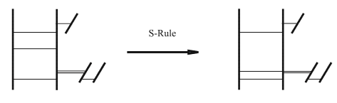
Figure 3: The brane moving between $D6$ excites some VEV for the quarks. Using the s-rule demands picking a particular point in the Coulomb branch moduli space.

In this picture, it is also clear that one has to go to a particular point of the Coulomb branch in which one of the color $D4$ is aligned with a flavor $D4$ so that we can have the recombination allowing for a supersymmetric Higgs branch. If we denote by $a^{\alpha}$ the positions of the color $D4$ and $m_{i}$ the positions of the flavor $D4$, the effective masses of the quarks are given by $M_{i}^{\alpha}=|a^{\alpha}-m_{i}|$. Consider first the case in which we have the full unbroken gauge group, and assume all the quark masses equal $m_{i}=m$. Then we can choose $a^{\alpha}=0$ and $M_{i}^{\alpha}=m$. This corresponds to having all the $D6$ at the same point in $5,6$ at a distance $m$ of the stack containing all the color $D4$. We can cut $k$ of the flavor $D4$ ending on a far brane and force them to end on a nearer brane. Then, we can move the resulting $D4$ pieces between the $D6$ giving VEV to some quarks. However, this would break the s-rule, so we need to pick $k$ of the color $D4$ and recombine them with the broken $D4$ so that each $NS$ is connected to each $D6$ with just one $D4$ according to the s-rule. But this will break the gauge group, since we are moving away $k$ color branes. Furthermore, in order to do this, we have to align the $D4$ branes, so we have to put the $k$ $D4$ at $a=m$ each aligned with a different cut flavor brane, in very much the same spirit as in the picture we found in our holographic setup, in which we also had to move $k$ of the color branes to recombine them with the flavor ones. It is interesting to note that also in this brane web setup the Higgs branch is realized by means of the recombination of the color branes with the flavor ones.

4.1.2 Fluctuations in $Dp-D(p+4)$ with flux

So far we have seen how we can realize the Higgs branch of the theory in the gravity side by means of dissolving some of the color branes in the flavor ones; providing an explicit route between field theory and gravity by means of the dielectric description. We will now turn back to the macroscopical description, and we will consider fluctuations around the instanton configuration; which will correspond to the meson spectrum in the Higgs branch of the gauge theory.

Since we have a similar situation for all the $Dp-D(p+4)$ intersections, namely a one to one correspondence between the Higgs phase of the corresponding field theory and the moduli space of instantons in four dimensions, in this section we will work with the general $Dp-D(p+4)$ system. Both the macroscopic and the microscopic analysis of the previous section can be extended in a straightforward manner to the general case, so we will first briefly sketch the macroscopical computation to set notations, and turn to the fluctuations.

The metric background (2.1) contains a dilaton given by (25) and a RR 4-form potential given by

$$C^{(p+1)}=\bigg{(}\frac{r^{2}}{R^{2}}\bigg{)}^{\alpha}dx^{0}\wedge\cdots\wedge dx^{p}\,,$$ (126)

where $\alpha$ is that in (26).

We will separate again the $\vec{r}$ coordinates in two sets, namely $\vec{r}=(\vec{y},\vec{z})$, where $\vec{y}$ has four components, and we will denote $\rho^{2}=\vec{y}\cdot\vec{y}$. As $r^{2}=\rho^{2}+\vec{z}^{2}$, the metric can be written as

$$ds^{2}=\bigg{(}\frac{\rho^{2}+\vec{z}^{2}}{R^{2}}\bigg{)}^{\alpha}dx_{1,p}^{2}+\bigg{(}\frac{R^{2}}{\rho^{2}+\vec{z}^{2}}\bigg{)}^{\alpha}(d\vec{y}^{2}+d\vec{z}^{2})\,.$$ (127)

In this background we will consider a stack of $N_{f}$ $D(p+4)$-branes extended along $(x^{\mu},\vec{y})$ at fixed distance $L$ in the transverse space spanned by the $\vec{z}$ coordinates (i.e. with $|\hskip 0.5pt\vec{z}\hskip 0.5pt|=L$). If $\xi^{a}=(x^{\mu},\vec{y})$ are the worldvolume coordinates, the action of a probe $D(p+4)$-brane is

$$S^{D(p+4)} = -T_{p+4}\int d^{\hskip 1.0ptp+5}\xi\,e^{-\phi}Str\big{\{}\sqrt{-\det(g+F)}\big{\}}$$ (128)

$${}+{T_{p+4}\over 2}\int Str\big{\{}P(C^{(p+1)})\wedge F\wedge F\big{\}}\,,$$

where $g$ is the induced metric and $F$ is the $SU(N_{f})$ worldvolume gauge field strength. In order to write $g$ more compactly, let us define the function $h$ as follows:

$$h(\rho)\equiv\bigg{(}\frac{R^{2}}{\rho^{2}+L^{2}}\bigg{)}^{\alpha}\,.$$ (129)

Then, one can write the nonvanishing elements of the induced metric as

$$g_{x^{\mu}x^{\nu}}={\eta_{\mu\nu}\over h}\,,\qquad g_{y^{i}y^{j}}=h\delta_{ij}\,.$$ (130)

Let us now assume that the only nonvanishing components of the worldvolume gauge field $F$ are those along the $y^{i}$ coordinates. Following the same steps as in (4.1), the action for the $D(p+4)$-brane probe can be written as

$$S^{D(p+4)}\,=\,-T_{p+4}\int\,d^{4}x\,d^{4}y\,\,{\rm Str}\,\Bigg{\{}\sqrt{\,1+{1\over 2}\,\Bigg{(}\frac{\rho^{2}\,+\,L^{2}}{R^{2}}\Bigg{)}^{2\alpha}F^{2}+\frac{1}{16}\Bigg{(}\frac{\rho^{2}\,+\,L^{2}}{R^{2}}\Bigg{)}^{4\alpha}\Big{(}\,{}^{*}FF\,\Big{)}^{2}}\,-\,$$

$$\qquad\qquad\qquad\qquad\qquad\qquad\qquad\qquad\,\,-\frac{1}{4}\Bigg{(}\,\frac{\rho^{2}\,+\,L^{2}}{R^{2}}\,\Bigg{)}^{2\alpha}\,\,{}^{*}FF\Bigg{\}}\,,$$ (131)

where $F^{2}$ and ${}^{*}FF$ are defined as in Eqs. (82) and (83). If, in addition, $F_{ij}$ is self-dual, one can check that the equations of motion of the gauge field are satisfied and, actually, there is a cancellation between the DBI and WZ parts of the action (131) generalizing (88), namely

$$S^{D(p+4)}\hbox{(self-dual)}=-T_{p+4}\int Str[1]=-N_{f}T_{p+4}\int d^{\hskip 1.0ptp+1}x\int d^{\hskip 0.5pt4}y\,.$$ (132)

We turn now to the analysis of the fluctuations around the self-dual configuration and the computation of the corresponding meson spectrum for this fluxed $Dp-D(p+4)$ intersection. Since the main particularity of this embedding corresponding to the Higgs branch is the presence of the worldvolume gauge field, following [63] and [65] we will focus on its fluctuations, for which we will write

$$A=A^{\rm inst}+a\,,$$ (133)

where $A^{\rm inst}$ is the gauge potential corresponding to a self-dual gauge field strength $F^{\rm inst}$ and $a$ is the fluctuation. The total field strength $F$ reads

$$F_{ab}=F^{\rm inst}_{ab}+f_{ab}\,,$$ (134)

with $f_{ab}$ being given by

$$f_{ab}=\partial_{a}a_{b}-\partial_{b}a_{a}+{1\over 2\pi\alpha^{\prime}}\,[A^{\rm inst}_{a},a_{b}]+{1\over 2\pi\alpha^{\prime}}\,[a_{a},A^{\rm inst}_{b}]+{1\over 2\pi\alpha^{\prime}}\,[a_{a},a_{b}]\,,\qquad$$ (135)

where the indices $a$, $b$ run now over all the worldvolume directions. Next, let us expand the action (128) in powers of the field $a$ up to second order. With this purpose in mind, we rewrite the square root in the DBI action as

$$\sqrt{-\det(g+F^{\rm inst}+f)}=\sqrt{-\det(g+F^{\rm inst})}\sqrt{\det(1+X)}\,,$$ (136)

where $X$ is the matrix

$$X\equiv(g+F^{\rm inst})^{-1}f\,.$$ (137)

We will expand the r.h.s. of (136) in powers of $X$ by using the equation

$$\sqrt{\det(1+X)}=1+{1\over 2}TrX-{1\over 4}TrX^{2}+{1\over 8}(TrX)^{2}+{\mathcal{O}}(X^{3})\,.$$ (138)

In our case, let us denote by ${\cal G}$ and ${\cal J}$ to the symmetric and antisymmetric part of the inverse of $X$, i.e.

$$X\,=\,\Big{(}\,g\,+\,F^{inst}\,\Big{)}^{-1}\,=\,{\cal G}\,+\,{\cal J}\,,\qquad{\cal G}^{\mu\nu}\,=\,h\,\,\eta^{\mu\nu}\,,\qquad{\cal G}^{ij}\,=\,{h\over H}\,\delta_{ij}\,,\qquad{\cal J}^{ij}\,=\,-{F^{inst}_{ij}\over H}\,;$$ (139)

where $h$ has been defined in (129) and the function $H$ is given by

$$H\equiv h^{2}+{1\over 4}\,(F^{\rm inst})^{2}\,.$$ (140)

The symmetric part ${\cal{G}}$ behaves as an “open string metric,” and it carries combined information from the worldvolume gauge field and metric.

By using these results we get, after a straightforward computation, the action up to quadratic order in the fluctuations; namely

$$S^{D(p+4)} = -T_{p+4}\int Str\bigg{\{}1+\frac{H}{4}f_{\mu\nu}f^{\mu\nu}+\frac{1}{2}\,f_{i\mu}f^{i\mu}+\frac{1}{4H}f_{ij}f^{ij}$$ (141)

$${}+\frac{1}{8h^{2}H}(F^{ij}f_{ij})^{2}-\frac{1}{4h^{2}H}\,F^{ij}F^{kl}f_{jk}f_{li}-\frac{1}{8h^{2}}\,f_{ij}f_{kl}\epsilon^{ijkl}\bigg{\}}\,,\qquad\$$

where we are dropping the superscript in the instanton field strength.

From now on we will assume again that $N_{f}=2$ and that the unperturbed configuration is the one-instanton $SU(2)$ gauge field written in Eq. (115). Moreover, we will focus on the subset of fluctuations for which $a_{i}=0$, i.e. on those for which the fluctuation field $a$ has nonvanishing components only along the Minkowski directions. However, we should impose this ansatz at the level of the equations of motion in order to ensure the consistency of the truncation. Let us consider first the equation of motion for $a_{i}$, which after imposing $a_{i}=0$ reduces to

$$D_{i}\partial^{\mu}a_{\mu}=0\,.$$ (142)

Moreover, the equation for $a_{\mu}$ when $a_{i}=0$ becomes

$$HD^{\mu}f_{\mu\nu}+D^{i}f_{i\nu}=0\,,$$ (143)

where now $H$ is given in (140), with $(F^{\rm inst})^{2}$ as in (118). Equation (142) is solved by requiring

$$\partial^{\mu}a_{\mu}=0\,.$$ (144)

Using this result, Eq. (143) can be written as

$$H\partial^{\mu}\partial_{\mu}a_{\nu}+\partial_{i}\partial_{i}a_{\nu}+\partial^{i}\bigg{[}{A_{i}\over 2\pi\alpha^{\prime}},a_{\nu}\bigg{]}$$

$$\qquad{}+\bigg{[}{A_{i}\over 2\pi\alpha^{\prime}},\partial_{i}a_{\nu}\bigg{]}+\bigg{[}{A_{i}\over 2\pi\alpha^{\prime}},\bigg{[}{A_{i}\over 2\pi\alpha^{\prime}},a_{\nu}\bigg{]}\bigg{]}=0\,.$$ (145)

Let us now adopt the following ansatz for $a_{\mu}$:

$$a_{\mu}^{(l)}=\xi_{\mu}(k)f(\rho)e^{ik_{\mu}x^{\mu}}\tau^{l}\,,$$ (146)

where $\tau^{l}$ is a Pauli matrix. This ansatz solves Eq. (144) provided the following transversality condition is fulfilled:

$$k^{\mu}\xi_{\mu}=0\,.$$ (147)

Moreover, one can check that, for this ansatz, one has

$$\partial^{i}\,\big{[}\,A_{i}\,,\,a_{\nu}^{(l)}\,\big{]}\,=\,\big{[}\,A_{i}\,,\partial_{i}a_{\nu}^{(l)}\,\big{]}\,=\,0\,\,,$$ (148)

$$\Big{[}\,{A_{i}\over 2\pi\alpha^{\prime}}\,,\Big{[}\,{A_{i}\over 2\pi\alpha^{\prime}}\,,a_{\nu}^{(l)}\Big{]}\Big{]}\,=\,-\,\frac{8\Lambda^{4}}{\rho^{2}(\rho^{2}+\Lambda^{2})^{2}}\,\,\xi_{\nu}(k)\,f(\rho)\,\,e^{ik_{\mu}x^{\mu}}\,\tau^{l}\,\,.$$ (149)

Let us now use these results in Eq. (145). Denoting $M^{2}=-k^{2}$ (which will be identified with the mass of the meson in the dual field theory) and using Eq. (118) to compute the function $H$ (see Eq. (140)), one readily reduces (145) to the following second-order differential equation for the function $f(\rho)$ of the ansatz (146):

$$\bigg{[}\frac{R^{4\alpha}M^{2}}{(\rho^{2}{+}L^{2})^{2\alpha}}\bigg{(}1{+}\frac{12(2\pi\alpha^{\prime})^{2}\Lambda^{4}}{R^{4\alpha}}\frac{(\rho^{2}{+}L^{2})^{2\alpha}}{(\rho^{2}{+}\Lambda^{2})^{4}}\bigg{)}{-}\frac{8\Lambda^{4}}{\rho^{2}(y^{2}{+}\Lambda^{2})^{2}}{+}\frac{1}{\rho^{3}}\partial_{\rho}(\rho^{3}\partial_{\rho})\bigg{]}f = 0\,.$$

In order to analyze Eq. (4.1.2), let us introduce a new radial variable $\varrho$ and a reduced mass $\bar{M}$, which are related to $\rho$ and $M$ as

$$\rho=L\varrho\,,\qquad\bar{M}^{2}=R^{7-p}L^{p-5}M^{2}\,.$$ (151)

Moreover, following [53], it is interesting to rewrite the fluctuation equation in terms of field theory quantities. Accordingly, let us introduce the quark mass $m_{q}$ and its VEV $v$ as follows:

$$m_{q}={L\over 2\pi\alpha^{\prime}}\,,\qquad v={\Lambda\over 2\pi\alpha^{\prime}}\,.$$ (152)

Notice that the relation between $v$ and the instanton size $\Lambda$ is consistent with our analysis in (4.2) (see Eq. (123)) and with the proposal of [63].

We can reexpress the equation for the fluctuations in terms of field theory quantities by means of (12) and (16), giving

$$\left[\frac{\bar{M}^{2}}{(1+\varrho^{2})^{2\alpha}}\left(1+c_{p}(v,m_{q})\,\frac{(1+\rho^{2})^{2\alpha}}{\Big{(}\varrho^{2}+\big{(}\frac{v}{m_{q}}\big{)}^{2}\Big{)}^{4}}\right)\right.$$

$$\left.\qquad{}-\bigg{(}\frac{v}{m_{q}}\bigg{)}^{4}\frac{8}{\varrho^{2}\Big{(}\varrho^{2}+\big{(}\frac{v}{m_{q}}\big{)}^{2}\Big{)}^{2}}+\frac{1}{\rho^{3}}\partial_{\varrho}(\varrho^{3}\partial_{\varrho})\right]f=0\,,$$ (153)

where $c_{p}(v,m_{q})$ is defined as

$$c_{p}(v,m_{q})\equiv\frac{12\cdot 2^{p-2}\pi^{\frac{p+1}{2}}}{\Gamma\big{(}\frac{7-p}{2}\big{)}}\,{v^{4}\over g_{\rm eff}^{2}(m_{q})m_{q}^{4}}\,.$$ (154)

Notice that everything conspires to absorb the powers of $\alpha^{\prime}$ and give rise to the effective coupling at the quark mass in $c_{p}(v,m_{q})$.

Equation (4.1.2) differs in the $\bar{M}$ term from the one obtained in [63], where the term proportional to $c_{p}(v,m_{q})$ is absent. We would like to point out that in order to arrive to (4.1.2) we expanded up to quadratic order in the fluctuations and we have kept all orders in the instanton field. The extra factor compared to that in [63] comes from the fact that, for a self-dual worldvolume gauge field, the unperturbed DBI action actually contains the square root of a perfect square, which can be evaluated exactly and shows up in the Lagrangian of the fluctuations. This extra term is proportional to the inverse of the effective Yang–Mills coupling. In order to ensure the validity of the DBI approximation, we should have slowly varying gauge fields, which further imposes that $F\wedge F$ should be much smaller than $\alpha^{\prime}$. Also, to trust the supergravity approximation, the effective Yang–Mills coupling should be large, which would suggest that the effect of this term is indeed negligible. However, in the region of small $\frac{v}{m_{q}}$ the full term is actually dominating in the IR region and determines the meson spectrum.

We have postponed the detailed analysis of the meson spectrum to the appendix. Let us mention that this meson spectrum is discrete, i.e. we have a mass gap for the mesons proportional to the quark mass also in this Higgs branch of the gauge theory. Interestingly, as one can see in the Appendix, the meson spectrum exhibits a so-called spectral flow. When the instanton size is varied, the masses of the mesons change in a very similar way as if the quantum numbers, instead of the instanton size, were changing. This is the so-called spectral flow phenomenon, which was first suggested in [63]. However, the small instanton region is somehow singular, and indeed one encounters that the masses appear to go to zero. In this singular point, the approximation is no longer valid, since the $F^{2}$ terms becomes basically a delta function. Indeed, at this point one should expect some sort of singular behavior, since there the VEV of the quark fields vanishes and the gauge group unhiggses; and one would expect that at this point new light degrees of freedom would enter the low energy description.

Let us now study the dependence of the mass gap as a function of the quark mass $m_{q}$ and the quark VEV $v$. First of all, we notice that the relation between the reduced mass $\bar{M}$ and the mass $M$ can be rewritten in terms of the quark mass $m_{q}$ and the dimensionless coupling constant $g_{\rm eff}(m_{q})$ as

$$M\propto{m_{q}\over g_{\rm eff}(m_{q})}\,\bar{M}\,.$$ (155)

For large $v$ the reduced mass $\bar{M}$ tends to a value independent of both $m_{q}$ and $v$. Thus, the meson mass $M$ depends only on $m_{q}$ in a holographic way, namely

$$M\sim{m_{q}\over g_{\rm eff}(m_{q})}\quad(v\to\infty)\,.$$ (156)

Notice that this dependence on $m_{q}$ and $v$ is exactly the same as in the unbroken symmetry case, although the numerical coefficient is different from that found in [52] and [53]. On the contrary, for small $v$, after combining Eq. (155) with the WKB result (352), we get that the mass gap depends linearly on $v$ and is independent on the quark mass $m_{q}$:

$$M\sim v\quad(v\to 0)\,,$$ (157)

and, in particular, the mass gap disappears in the limit $v\to 0$, which corresponds to having a zero size instanton.

4.2 The codimension one defect

We will now consider the intersection of $Dp$- and $D(p+2)$-branes according to the array:

$$\begin{array}[]{rcccccccccl}&1&\cdots&p-1&p&p+1&p+2&p+3&\cdots&9&\\[2.0pt] Dp:&\times&\cdots&\times&\times&-&-&-&\cdots&-&\\[2.0pt] D(p+2):&\times&\cdots&\times&-&\times&\times&\times&\cdots&-&\end{array}$$

Clearly, this defines a codimension 1 defect in the bulk $p$-dimensional gauge theory where the matter is confined.

Exactly as in the codimension 0 defect, from the gravity point of view, also in this case all the dimensionalities behave in a similar way. However, we will study in a detailed way the $p=3$ case, where both the field theory and gravity descriptions will be analyzed. Since all the other dimensionalities behave similarly, when computing the spectrum we will do it in a unified manner for all $p$.

4.2.1 A case study II$:$ the $D3-D5$ intersection

Since the dual field theory to the $D3-D5$ intersection is somehow less familiar, we will start with the gravity description in order to gain some intuition on the dynamics of the system. The study of the Coulomb branch of this system was initiated in [69] and further pursued in [52] and [71]; where an interpretation of the gravity dual of the Higgs branch was given. In Sec. 3 we discussed the Coulomb branch, and we now turn to the Higgs branch of the system. For that, let us split the six transverse coordinates $\vec{y}$ to the color $D3$ branes in two sets of three elements, according to the $D3-D5$ intersection represented by the array (4.2). The coordinates $(y^{1},y^{2},y^{3})$ are those which are parallel to the $D5$-brane worldvolume in (4.2). It is convenient to go to spherical coordinates as $(dy^{1})^{2}+(dy^{2})^{2}+(dy^{3})^{2}=d\rho^{2}+\rho^{2}d\Omega_{2}^{2}$, where $d\Omega_{2}^{2}$ is the line element of a unit two-sphere. Moreover, let us denote by $\vec{z}=(z^{1},z^{2},z^{3})=(y^{4},y^{5},y^{6})$ the coordinates transverse to both the $D3$- and $D5$-branes. Clearly, $r^{2}=\rho^{2}+\vec{z}^{2}$, so the background $AdS_{5}\times S^{5}$ metric can be written as

$$ds^{2}={\rho^{2}+\vec{z}^{2}\over R^{2}}\,dx_{1,3}^{2}+{R^{2}\over\rho^{2}+\vec{z}^{2}}(d\rho^{2}+\rho^{2}\,d\Omega_{2}^{2}+d\vec{z}\cdot d\vec{z})\,.$$ (159)

Since our probe flavor branes will be $D5$ branes partially overlapping the $D3$, in order to couple the background 4-form potential we have to turn on a nonzero worldvolume magnetic field. In this case, the action to be considered is

$$S_{D5}=-T_{5}\int d^{\hskip 0.5pt6}\xi\sqrt{-\det(g+F)}+T_{5}\int d^{\hskip 0.5pt6}\xi\,P[C^{(4)}]\wedge F\,,$$ (160)

where $g$ is the pullback of the metric (159), $F$ is the strength of the Abelian worldvolume gauge field and $\xi^{a}$ $(a=0,\ldots,5)$ are a set of worldvolume coordinates. In what follows we will use $x^{0}$, $x^{1}$, $x^{2}$ and the radial ($\rho$) and angular coordinates of Eq. (159) as our set of worldvolume coordinates.

Generically, the embedding of the $D5$-brane probe is then specified by the values of $x^{3}$ and $\vec{z}$ as functions of the $\xi^{a}$’s. We will consider static embeddings in which $|\vec{z}|$ is a fixed constant, namely $|\vec{z}|=L$. The simplest of such embeddings is the one in which the coordinate $x^{3}$ is also a constant. In this case, it is clear from (160) that the WZ coupling will vanish independently of $F$, since in order to capture the RR potential we need a nontrivial $x^{3}$ dependence so that the pull-back in (160) does not vanish. Therefore, for constant $x^{3}$ we can take the worldvolume gauge field $F$ to vanish. This corresponds to the Coulomb branch of the dual theory. Since the defect lives at a fixed $x^{3}$ position, it represents a domain wall in the four-dimensional Minkowski.

In turn, if we are to couple the 4-form potential, we need to consider a nontrivial $x^{3}$ dependence on the worldvolume coordinates. This demands to turn a nonzero magnetic $F$ along the two-sphere of its worldvolume. To be precise, let us assume that $F$ is given by

$$F=qVol(S^{2})\equiv{\cal F}\,,$$ (161)

where $q$ is a constant and $Vol(S^{2})$ is the volume form of the worldvolume two-sphere. To understand the implications of having a magnetic flux across the worldvolume $S^{2}$, let us look at the form of the Wess–Zumino term in the action (160), which will involve

$$S_{\rm WZ}\sim\int_{S^{2}}F\int P[C^{(4)}]\sim qx^{\prime}\,,$$ (162)

where $x\equiv x^{3}$ and the prime denotes the derivative with respect to the radial coordinate $\rho$. It is clear from (162) that the worldvolume flux acts as a source of a nontrivial dependence of $x$ on the coordinate $\rho$. Assuming that $x$ only depends on $\rho$, the action (160) of the probe takes the form:

$$S_{D5}=-4\pi\,T_{5}\,\int\,d^{3}x\,d\rho\Bigg{[}\,\rho^{2}\,\sqrt{1\,+\,{(\rho^{2}+L^{2})^{2}\over R^{4}}\,x^{\prime\,2}}\,\,\sqrt{1\,+\,{(\rho^{2}+L^{2})^{2}\over R^{4}}\,{q^{2}\over\rho^{4}}}\,\,-\,\,{(\rho^{2}+L^{2})^{2}\over R^{4}}\,q\,x^{\prime}\,\Bigg{]}\,\,,$$ (163)

where we have assumed that $\vec{z}$ is constant ($|\hskip 0.5pt\vec{z}\hskip 0.5pt|=L$) and we have integrated over the coordinates of the two-sphere. The Euler–Lagrange equation for $x(\rho)$ derived from (163) is quite involved. However, there is a simple first-order equation for $x(\rho)$ which solves this equation [72], namely

$$x^{\prime}(\rho)={q\over\rho^{2}}\,.$$ (164)

Actually, the first-order equation (164) is a BPS equation required by supersymmetry, as can be verified by checking the kappa symmetry of the embedding [72]. The integration of Eq. (164) is straightforward:

$$x(\rho)=x_{0}-{q\over\rho}\,,$$ (165)

where $x_{0}$ is an integration constant. The dependence on $\rho$ of the r.h.s. of Eq. (165) represents the bending of the $D5$-brane profile required by supersymmetry when there is a nonvanishing flux of the worldvolume gauge field. Notice also that now the probe is located at a fixed value of $x$ only at the asymptotic value $\rho\to\infty$, whereas when $\rho$ varies the $D5$-brane fills one-half on the worldvolume of the $D3$-brane (i.e. $x^{3}\leq x_{0}$ for $q>0$). Actually, this indicates that this embedding corresponds not to a deformation of the theory, but rather to a choice of vacuum. The reason is that both the embedding at constant $x$ and the bended one share the same asymptotics, so one would expect that they correspond to different vacua rather than to a deformation of the boundary theory. We will explicitly see that it is indeed the case when studying the system from the dual field theory side; where we will explicitly see, along the lines in the codimension zero case, that the gauge theory contains both the Coulomb and Higgs branch we studied.

It is interesting to study the modifications of the induced metric introduced by the bending. Actually, when $q\not=0$ this induced metric takes the form

$${\cal G}_{ab}\,d\xi^{a}\,d\xi^{b} = {\rho^{2}+L^{2}\over R^{2}}\,dx^{2}_{1,2}+{R^{2}\over\rho^{2}+L^{2}}\bigg{[}\bigg{(}1+{q^{2}\over R^{4}}\,{(\rho^{2}+L^{2})^{2}\over\rho^{4}}\bigg{)}d\rho^{2}+\rho^{2}\,d\Omega_{2}^{2}\bigg{]}\,.$$

In the $L=0$ case, the metric reduces to an effective $AdS_{4}$ worldvolume. Therefore, like in the Coulomb phase, the dual theory enjoys a conformal symmetry even in the Higgs phase. However, even in the $L\neq 0$ case, the UV metric at $\rho\to\infty$ takes the same form, since in the UV the quark mass is completely irrelevant and thus theory asymptotes to a conformal one. Considering the generic massive case, the worldvolume induced metric is

$$AdS_{4}(R_{\rm eff})\times S^{2}(R)\,,$$ (167)

where the radius of the $AdS_{4}$ changes from its fluxless value $R$ to $R_{\rm eff}$, with the latter given by:

$$R_{\rm eff}=\bigg{(}1+{q^{2}\over R^{4}}\bigg{)}^{{1\over 2}}\,R\,.$$ (168)

Notice that the radius of the $S^{2}$ is not affected by the flux, as is clear from (LABEL:ind-met-flux).

One can understand the appearance of this UV metric as follows. Let us suppose that we have an $AdS_{5}$ metric of the form

$$ds^{2}_{AdS_{5}}={\rho^{2}\over R^{2}}\,dx^{2}_{1,3}+{R^{2}\over\rho^{2}}\,d\rho^{2}\,.$$ (169)

Let us now change variables from $(\rho,x^{3})$ to new coordinates $(\varrho,\eta)$:

$$x^{3}=\bar{x}-{\tanh\eta\over\varrho}\,,\qquad\rho=R^{2}\varrho\cosh\eta\,,$$ (170)

where $\bar{x}$ is a constant. It can be easily seen that the $AdS_{5}$ metric (169) in the new variables takes the form

$$ds^{2}_{AdS_{5}}=R^{2}(\cosh^{2}\eta\,ds^{2}_{AdS_{4}}+d\eta^{2})\,,$$ (171)

where $ds^{2}_{AdS_{4}}$ is the metric of $AdS_{4}$ with unit radius, given by

$$ds^{2}_{AdS_{4}}=\varrho^{2}\,dx^{2}_{1,2}+{d\varrho^{2}\over\varrho^{2}}\,.$$ (172)

The first equation in (170), when written in terms of $\rho$, reads

$$x=\bar{x}-\frac{R^{2}\sinh\eta}{\rho}\,,$$ (173)

which is exactly (165) once we identify $q=R^{2}\sinh\eta$. Thus, our embedding corresponds to fixed $\eta$ slices of the original $AdS_{5}$, and thus should correspond to an $AdS_{4}$ worldvolume with effective radius

$$R_{\rm eff}=R\cosh\eta\,.$$ (174)

The worldvolume gauge field (161) is constrained by a flux quantization condition [94] which, with our notations, reads

$$\int_{S^{2}}F={2\pi k\over T_{f}}\,,\qquad k\in Z\,,\qquad T_{f}={1\over 2\pi\alpha^{\prime}}\,.$$ (175)

It is now immediate to conclude that the condition (175) restricts the constant $q$ to be of the form:

$$q=k\pi\alpha^{\prime}\,,$$ (176)

where $k$ is an integer.

A microscopical picture

The presence of a worldvolume flux as in (161) induces, through the Wess–Zumino term of the action (160), a $D3$-brane charge, proportional to $\int_{S^{2}}\,F$, on the $D5$-brane. Indeed, we can think again the system as a recombination of some of the color branes with the flavor ones. For this reason it is not surprising that this $D5$-brane configuration admits also a microscopical description in terms of a bound state of coincident $D3$-branes. Actually, the integer $k$ of the quantization condition (175) has the interpretation of the number of $D3$-branes that build up the $D5$-brane. The dynamics of a stack of coincident $D3$-branes is determined by the Myers dielectric action [68] (see Appendix).

The Wess–Zumino term for the $D3$-brane under consideration is

$$S_{\rm WZ}^{D3}=T_{3}\int d^{\hskip 0.5pt4}\xi Str\big{[}P\big{[}C^{(4)}\big{]}\big{]}\,.$$ (177)

Let us now choose $x^{0}$, $x^{1}$, $x^{2}$ and $\rho$ as our set of worldvolume coordinates of the $D3$-branes. Moreover, we shall introduce new coordinates $Y^{I}(I=1,2,3)$ for the two-sphere of the metric (159). These new coordinates satisfy $\sum_{I}Y^{I}Y^{I}=1$ and the line element $d\Omega_{2}^{2}$ is given by

$$d\Omega_{2}^{2}=\sum_{I}\,dY^{I}\,dY^{I}\,,\qquad\sum_{I}\,Y^{I}Y^{I}=1\,.$$ (178)

We will assume that the $Y^{I}$’s are the only noncommutative scalars. They will be represented by $k\times k$ matrices. In this case the matrix $Q$ appearing in (94) is given by

$$Q_{J}^{I}=\delta_{J}^{I}+{i\over 2\pi\alpha^{\prime}}\,[Y^{I},Y^{K}]G_{KJ}\,.$$ (179)

Actually, we shall adopt the ansatz in which the $Y^{I}$’s are constant and given by

$$Y^{I}={J^{I}\over\sqrt{C_{2}(k)}}\,,$$ (180)

where the $k\times k$ matrices $J^{I}$ correspond to the $k$-dimensional irreducible representation of the $SU(2)$ algebra:

$$[J^{I},J^{J}]=2i\epsilon_{IJK}J^{K}\,,$$ (181)

and $C_{2}(k)$ is the quadratic Casimir of the $k$-dimensional irreducible representation of $SU(2)$ ($C_{2}(k)=k^{2}-1$). Then, the $Y^{I}$ satisfy

$$Y^{I}Y^{I}=1$$ (182)

as a matrix identity, and therefore, the $Y^{I}$ scalars parametrize a fuzzy two-sphere. Moreover, let us assume that we consider embeddings in which the scalars $\vec{z}$ and $x^{3}$ are commutative and such that $|\vec{z}|=L$ and $x^{3}=x(\rho)$ (a unit $k\times k$ matrix is implicit). With these conditions, as the metric (159) does not mix the directions of the two-sphere with the other coordinates, the matrix $Q^{-1}-\delta$ does not contribute to the first square root on the r.h.s. of (94). Then

$$\sqrt{-\det\big{[}P[G]\,\big{]}}={\rho^{2}+L^{2}\over R^{2}}\,\sqrt{1+{(\rho^{2}+L^{2})^{2}\over R^{4}}\,x^{\prime 2}}\,.$$ (183)

Moreover, by using the ansatz (180) and the commutation relations (181) we obtain that, for large $k$, the second square root appearing in (94) can bewritten as

$$Str\big{[}\sqrt{\det Q}\big{]}\approx{R^{2}\over\pi\alpha^{\prime}}\,{\rho^{2}\over\rho^{2}+L^{2}}\,\sqrt{1+{(\rho^{2}+L^{2})^{2}\over R^{4}}\,{(k\pi\alpha^{\prime})^{2}\over\rho^{4}}}\,.$$ (184)

Using these results, the DBI part of the $D3$-brane action in this large $k$ limit takes the form

$$S_{\rm BI}^{D3}=-{T_{3}\over\pi\alpha^{\prime}}\int d^{\hskip 0.5pt3}x\,d\rho\,\rho^{2}\sqrt{1+{(\rho^{2}+L^{2})^{2}\over R^{4}}\,x^{\prime 2}}\sqrt{1+{(\rho^{2}+L^{2})^{2}\over R^{4}}\,{q^{2}\over\rho^{4}}}\,,\quad$$ (185)

where we have already used (176) to write the result in terms of $q$. Due to the relation $T_{3}=4\pi^{2}\alpha^{\prime}T_{5}$ between the tensions of the $D3$- and $D5$-branes, one checks by inspection that the r.h.s. of (185) coincides with the Born–Infeld term of the $D5$-brane action (163). Notice also that the quantization integer $k$ in (175) is identified with the number of $D3$-branes. Moreover, the Wess–Zumino term (177) becomes

$$S_{\rm WZ}^{D3}=kT_{3}\int d^{\hskip 0.5pt3}x\,d\rho\,{(\rho^{2}+L^{2})^{2}\over R^{4}}\,x^{\prime}\,.$$ (186)

The factor $k$ in (186) comes from the trace of the unit $k\times k$ matrix.

By comparing (186) with the Wess–Zumino term of the macroscopical action (163) one readily concludes that they coincide; since because of (176) we have that $4\pi qT_{5}=kT_{3}$.

Field theory analysis

The field theory dual to the $D3-D5$ intersection has been worked out by DeWolfe et al. in [69] (see also [70]). Let us consider for simplicity the massless case. Then, the theory, which includes ${\mathcal{N}}=4$ $SU(N)$ $SYM$ in four-dimensional plus an ${\cal N}=4$ hypermultiplet confined to the defect, has an $SU(2)_{H}\times SU(2)_{V}$ R-symmetry. The $SU(2)_{H}$ ($SU(2)_{V}$) symmetry corresponds to the rotations in the 456 (789) directions of the array (4.2). Written in terms of ${\mathcal{N}}=1$ SUSY, this hypermultiplet gives rise to a chiral ($Q$) and an antichiral ($\bar{Q}$) supermultiplet, which are both doublets under $SU(2)_{H}$ while being in the fundamental representation of the gauge group. In addition, the six scalars of the bulk ${\mathcal{N}}=4$, which are in the adjoint of the gauge group, naturally split in two sets, the first (which we will call $\phi_{H}^{I}$) forming a vector of $SU(2)_{H}$ and the second, which we denote by $\phi_{V}^{A}$, a vector of $SU(2)_{V}$. Thus, the bosonic content of the theory is as follows:

Field	$SU(N)$	$SU(2)_{H}$	$SU(2)_{V}$
$A_{\mu}$	adjoint	singlet	singlet
$\phi_{H}^{I}$	adjoint	vector	singlet
$\phi_{V}^{A}$	adjoint	singlet	vector
$q$	fundamental	doublet	singlet
$\bar{q}$	fundamental	doublet	singlet

We will assume that only the fields $\phi_{H}$, $\phi_{V}$, $q$ and $\bar{q}$ are nonvanishing. The defect action for this theory has a potential term which can be written as [69]

$$S_{\rm defect} = -\frac{1}{g^{2}}\int d^{\hskip 0.5pt3}x\bigg{[}\bar{q}^{m}(\phi_{V}^{A})^{2}q^{m}+\frac{i}{2}\,\epsilon_{IJK}\bar{q}^{m}\sigma_{mn}^{I}[\phi_{H}^{J},\phi_{H}^{K}]q^{n}\bigg{]}$$ (187)

$${}-\frac{1}{g^{2}}\int d^{\hskip 0.5pt3}x\bigg{[}\bar{q}^{m}\sigma_{mn}^{I}\partial_{3}\phi_{H}^{I}q^{n}+\frac{1}{2}\,\delta(x_{3})(\bar{q}^{m}\sigma_{mn}^{I}T^{a}q^{n})^{2}\bigg{]}\,,\quad$$

where the integration is performed over the $x^{3}=0$ three-dimensional submanifold and $g$ is the Yang–Mills coupling constant.

For the supersymmetric configurations we are looking for, the potential term must vanish. One way to achieve this is to consider the quark fields to zero; and the $\Phi_{H}$, $\Phi_{V}$ fields to be commuting fields. The eigenvalues of the adjoint scalars parametrize, once again, the Coulomb branch of the theory, which in general involves a broken gauge group.

However, we can have more involved situations. Focusing on the equation of motion for the $\tilde{q}$ field, we have that

$$\phi_{V}q=0\,.$$ (188)

We can insure this property by taking $q$ as

$$q=\left(\begin{array}[]{c}0\\ \vdots\\ 0\\ \alpha_{1}\\ \vdots\\ \alpha_{k}\end{array}\right)\,,$$ (195)

and by demanding that $\phi_{V}$ is of the form

$$\phi_{V}=\left(\begin{array}[]{@{\hspace{1pt}}cc@{\hspace{1pt}}}\hskip 1.0pt\lx@intercol\hfil A&0\hfil\hskip 1.0\\ \hskip 1.0pt\lx@intercol\hfil 0&0\hfil\hskip 1.0\end{array}\right)\,,$$ (198)

where $A$ is an $(N-k)\times(N-k)$ traceless matrix. Moreover, we shall take $\phi_{V}$, $q$ and $\bar{q}$ constant, which is enough to guarantee that their kinetic energy vanishes. Notice that the scalars $\phi_{V}$ correspond to the directions 789 in the array (4.2), which are orthogonal to both the $D3$- and $D5$-brane. Note that, in a similar manner to the $D3-D7$ case, we have to pick a particular configuration for the transverse scalars to the system, corresponding in this case to the $\phi_{V}$. Therefore, we also need to go to a particular point in the Coulomb branch to enter the Higgs branch, and indeed, had we chosen a nonzero mass for the quarks, we would have had that some of the $\Phi_{V}$ eigenvalues should have been adjusted to cancel the mass term in order to enter the Higgs branch.

In order to find the supersymmetric vacua, let us consider the configurations of $\phi_{H}$ with vanishing energy. First of all we will impose that $\phi_{H}$ is a matrix whose only nonvanishing entries are in the lower $k\times k$ block. In this way the mixing terms of $\phi_{V}$ and $\phi_{H}$ cancel. Moreover, assuming that $\phi_{H}$ only depends on the coordinate $x^{3}$, the surviving terms in the bulk action are [69]

$$S_{\rm bulk}=-{1\over g^{2}}\int d^{\hskip 0.5pt4}xTr\bigg{[}{1\over 2}\,(\partial_{3}\phi_{H}^{I})^{2}-{1\over 4}\,[\phi_{H}^{I},\phi_{H}^{J}]^{2}\bigg{]}\,,$$ (199)

where the trace is taken over the color indices. It turns out that the actions (187) and (199) can be combined in such a way that their sum can be written as an integral over the four-dimensional space–time of the trace of a square. In order to write this expression, let us define the matrix $\alpha^{I}=\alpha^{Ia}T^{a}$, where the $T^{a}$’s are the generators of the gauge group and the $\alpha^{Ia}$’s are defined as the following expression bilinear in $q$ and $\bar{q}$:

$$\alpha^{Ia}\equiv\bar{q}^{m}\sigma_{mn}^{I}T^{a}q^{n}\,.$$ (200)

It is now straightforward to check that the sum of (187) and (199) can be put as

$$S_{\rm defect}+S_{\rm bulk}=-{1\over 2g^{2}}\int d^{\hskip 0.5pt4}xTr\bigg{[}\partial_{3}\phi_{H}^{I}+{i\over 2}\,\epsilon_{IJK}[\phi_{H}^{J},\phi_{H}^{K}]+\alpha^{I}\delta(x^{3})\bigg{]}^{2}\,,\qquad\$$ (201)

where we have used the fact that $\epsilon_{IJK}Tr\big{(}\partial_{3}\phi_{H}^{I}[\phi_{H}^{J},\phi_{H}^{K}]\big{)}$ is a total derivative with respect to $x^{3}$ and, thus, can be dropped if we assume that $\phi_{H}$ vanishes at $x^{3}=\pm\infty$. It is now clear from (201) that we must require the Nahm equations [95]:

$$\partial_{3}\phi_{H}^{I}+{i\over 2}\,\epsilon_{IJK}[\phi_{H}^{J},\phi_{H}^{K}]+\alpha^{I}\delta(x^{3})=0\,.$$ (202)

(For a nice review of the Nahm construction in string theory see [87] and [88].)

Notice that when $\alpha^{I}$ vanishes, Eq. (202) admits the trivial solution $\phi_{H}=0$. On the contrary, as shown in [71], if the fundamentals $q$ and $\bar{q}$ acquire a nonvanishing vacuum expectation value as in (195), $\alpha^{I}$ is generically nonzero and the solution of (202) must be nontrivial. Actually, it is clear from (202) that in this case $\phi_{H}$ must blow up at $x^{3}=0$, which shows how a nonvanishing vacuum expectation value of the fundamentals acts as a source for the brane recombination in the Higgs branch of the theory. Actually, away from $x_{3}=0$, the $\delta$-function term is zero, so we can consider just

$$\partial_{3}\phi_{H}^{I}+{i\over 2}\,\epsilon_{IJK}[\phi_{H}^{J},\phi_{H}^{K}]=0\,.$$ (203)

We shall adopt the ansatz

$$\phi_{H}^{I}(x)=f(x)\phi_{0}^{I}\,,$$ (204)

where $x$ stands for $x^{3}$ and $\phi_{0}^{I}$ are constant matrices. The differential equation (203) reduces to

$${f^{\prime}\over f^{2}}\,\phi_{0}^{I}+{i\over 2}\,\epsilon_{IJK}[\phi_{0}^{J},\phi_{0}^{K}]=0\,,$$ (205)

where the prime denotes derivative with respect to $x$. We shall solve this equation by first putting

$$\phi_{0}^{I}={1\over\sqrt{C_{2}(k)}}\left(\begin{array}[]{@{\hspace{2pt}}cc@{\hspace{0.8pt}}}\hskip 2.0pt\lx@intercol\hfil 0&0\hfil\hskip\\ \hskip 2.0pt\lx@intercol\hfil 0&J^{I}\hfil\hskip\end{array}\right)\,,$$ (208)

where the $J^{I}$ are matrices in the $k$-dimensional irreducible representation of the $SU(2)$ algebra, which satisfy the commutation relations (181), and we have normalized the $\phi_{0}^{I}$’s such that $\phi_{0}^{I}\phi_{0}^{I}$ is the unit matrix in the $k\times k$ block. By using this representation of the $\phi_{0}^{I}$’s, Eq. (205) reduces to

$${f^{\prime}\over f^{2}}={2\over\sqrt{C_{2}(k)}}\,,$$ (209)

which can be immediately integrated, namely

$$f=-{\sqrt{C_{2}(k)}\over 2x}\,.$$ (210)

For large $k$, the quadratic Casimir $C_{2}(k)$ behaves as $k^{2}$ and this equation reduces to

$$f=-{k\over 2x}\,.$$ (211)

Let us now take into account the standard relation between coordinates $X_{H}^{I}$ and scalar fields $\phi^{I}_{H}$, namely

$$X_{H}^{I}=2\pi\alpha^{\prime}\phi^{I}_{H}\,,$$ (212)

and the fact that $\rho^{2}\equiv X_{H}^{I}X_{H}^{I}$. Using these facts we immediately get the following relation between $\rho$ and $f$:

$$\rho=2\pi\alpha^{\prime}f\,,$$ (213)

and the solution (211) of the Nahm equation can be written as

$$\rho=-{\pi k\alpha^{\prime}\over x}\,,$$ (214)

which, if we take into account the quantization condition (176), is just our embedding (165) for $x_{0}=0$. As expected, $\rho$ blows up at $x=0$, while its dependence for $x\not=0$ gives rise to the same bending as in the brane approach. Now we can understand the $\delta$ term in (202), since it is precisely this term the one taking care of the blow-up of the solution at $x=0$. Notice also that, in this field theory perspective, the integer $k$ is the rank of the gauge theory subgroup in which the Higgs branch of the theory is realized, which corresponds to the number of $D3$-branes that recombine into a $D5$-brane.

4.2.2 Fluctuations in $Dp-D(p+2)$ with flux

Let us now study the fluctuations around the codimension one defect. As in the codimension 0 case, we can give a systematic treatment of all the $Dp-D(p+2)$ intersection with flux, which in turn behave similarly to the $D3-D5$ case studied above. Without loss of generality we can take the unperturbed configuration as $z^{1}=L$, $z^{m}=0$ $(m>1)$. Next, let us consider a fluctuation of the type:

$$\begin{array}[]{c}z^{1}=L+\chi^{1}\,,\qquad z^{m}=\chi^{m}\quad(m=2,\ldots,6-p)\,,\\[5.0pt] x^{p}={\cal X}+x\,,\qquad F={\cal F}+f\,,\end{array}$$ (217)

where the bending ${\cal X}$ and the worldvolume gauge field ${\cal F}$ are given by Eqs. (165) and (161) respectively and we assume that $\chi^{m}$, $x$ and $f$ are small. It is important to say that even for generic $p$ the bending is that of the $D3-D5$ case, being the reason that we are always considering the same codimensionality for the defect. Since this background, in addition to the presence of the worldvolume gauge field, involves the bending, it is interesting to consider the whole set of fluctuations.

The induced metric on the $D(p+2)$-brane worldvolume can be written as

$$g={\cal G}+g^{(f)}\,,$$ (218)

with ${\cal G}$ being the induced metric of the unperturbed configuration:

$${\cal G}_{ab}\,d\xi^{a}\,d\xi^{b}=h^{-1}\,dx_{1,p-1}^{2}+h\bigg{[}\bigg{(}1+{q^{2}\over\rho^{4}h^{2}}\bigg{)}d\rho^{2}+\rho^{2}\,d\Omega_{2}^{2}\bigg{]}\,,$$ (219)

where $h=h(\rho)$ is the function defined in (129). Moreover, $g^{(f)}$ is the part of $g$ that depends on the derivatives of the fluctuations, namely

$$g^{(f)}_{ab}={q\over\rho^{2}h}\,(\delta_{a\rho}\partial_{b}x+\delta_{b\rho}\partial_{a}x)+{1\over h}\,\partial_{a}x\partial_{b}x+h\partial_{a}\chi^{m}\partial_{b}\chi^{m}\,.$$ (220)

Let us next rewrite the Born–Infeld determinant as

$$\sqrt{-\det(g+F)}=\sqrt{-\det({\cal G}+{\cal F})}\sqrt{\det(1+X)}\,,$$ (221)

where the matrix $X$ is given in this case by

$$X\equiv({\cal G}+{\cal F})^{-1}\big{(}g^{(f)}+f\big{)}\,.$$ (222)

We shall evaluate the r.h.s. of (221) by expanding it in powers of $X$ by means of Eq. (138). In order to evaluate more easily the trace of the powers of $X$ appearing on the r.h.s. of this equation, let us separate the symmetric and antisymmetric part in the inverse of the matrix ${\cal G}+{\cal F}$:

$$({\cal G}+{\cal F})^{-1}=\hat{\cal G}^{-1}+{\cal J}\,,$$ (223)

where

$$\hat{\cal G}^{-1}\equiv{1\over({\cal G}+{\cal F})_{S}}\,,\qquad{\cal J}\equiv{1\over({\cal G}+{\cal F})_{A}}\,.$$ (224)

Notice that $\hat{\cal G}$ is just the open string metric which, generalizing for any $p$ (LABEL:ind-met-flux), is given by

$$\hat{\cal G}_{ab}\,d\xi^{a}\,d\xi^{b}=h^{-1}\,dx_{1,p-1}^{2}+h\bigg{(}1+{q^{2}\over\rho^{4}h^{2}}\bigg{)}(d\rho^{2}+\rho^{2}\,d\Omega_{2}^{2})\,.$$ (225)

Moreover, the antisymmetric matrix ${\cal J}$ takes the form

$${\cal J}^{\theta\varphi}=-{\cal J}^{\varphi\theta}=-{1\over\sqrt{\tilde{g}}}\,{q\over q^{2}+\rho^{4}h^{2}}\,,$$ (226)

where $\theta$, $\varphi$ are the standard polar coordinates on $S^{2}$ and $\tilde{g}=\sin^{2}\theta$ is the determinant of its round metric.

After some algebra, one has that, dropping constant global factors that do not affect the equations of motion, the relevant Lagrangian for the fluctuations is

$${\cal L} = -\rho^{2}\sqrt{\tilde{g}}\,\bigg{[}{h\over 2}\bigg{(}1+{q^{2}\over\rho^{4}h^{2}}\bigg{)}\hat{\cal G}^{ab}\partial_{a}\chi^{m}\partial_{b}\chi^{m}$$ (227)

$${}+{1\over 2h}\,\hat{\cal G}^{ab}\partial_{a}x\partial_{b}x+{1\over 4}\bigg{(}1+{q^{2}\over\rho^{4}h^{2}}\bigg{)}f_{ab}f^{ab}\bigg{]}-{C(\rho)\over 2}\,x\epsilon^{ij}f_{ij}\,,$$

where the indices $a$, $b$ are raised with the open string metric $\hat{\cal G}$, and where we have made use of the Bianchi identity for the gauge field fluctuations $\epsilon^{ij}\partial_{i}f_{j\rho}+\break{\epsilon^{ij}\over 2}\partial_{\rho}f_{ij}=0$. Finally, the functions $A(\rho)$, $C(\rho)$ are

$$A(\rho)=\frac{d}{d\rho}\bigg{[}\frac{q^{2}}{h^{2}(q^{2}+\rho^{4}h^{2})}\bigg{]}\,,\qquad C(\rho)=\frac{d}{d\rho}\bigg{[}\frac{\rho^{4}}{q^{2}+\rho^{4}h^{2}}\bigg{]}\,.$$ (228)

As it is manifest from (227), the transverse scalars $\chi$ do not couple to other fields, while the scalar $x$ is coupled to the fluctuations $f_{ij}$ of the gauge field strength along the two-sphere. For simplicity we will restrict to the $\chi$ sector from now on, although a complete analysis can be found in [71] and [65]. For the fluxless case $q=0$ these equations were solved in [52], where it was shown that they give rise to a discrete meson mass spectrum, which can be computed numerically and, in the case of the $D3-D5$ intersection, analytically. Let us examine here the situation for $q\not=0$. The equation of motion for $\chi$ that follow from (227) is

$$\partial_{a}\bigg{[}\sqrt{\tilde{g}}\rho^{2}h\bigg{(}1+{q^{2}\over\rho^{4}h^{2}}\bigg{)}\hat{\cal G}^{ab}\partial_{b}\chi\bigg{]}=0\,.$$ (229)

By using the explicit form of the open string metric $\hat{\cal G}^{ab}$ (Eq. (225)), we can rewrite (229) as

$$\partial_{\rho}(\rho^{2}\partial_{\rho}\chi)+\bigg{[}\rho^{2}h^{2}+{q^{2}\over\rho^{2}}\bigg{]}\partial^{\mu}\partial_{\mu}\chi+\nabla^{i}\nabla_{i}\chi=0\,.$$ (230)

Let us separate variables and write the scalars in terms of the eigenfunctions of the Laplacian in the Minkowski and sphere parts of the brane geometry as

$$\chi=e^{ikx}Y^{l}(S^{2})\xi(\rho)\,,$$ (231)

where the product $kx$ is performed with the Minkowski metric and $l$ is the angular momentum on the $S^{2}$. The fluctuation equation for the function $\xi$ is

$$\partial_{\rho}(\rho^{2}\partial_{\rho}\xi)+\bigg{\{}\bigg{[}R^{4\alpha}\,\frac{\rho^{2}}{(\rho^{2}+L^{2})^{2\alpha}}+\frac{q^{2}}{\rho^{2}}\bigg{]}M^{2}-l(l+1)\bigg{\}}\xi=0\,,$$ (232)

where $M^{2}=-k^{2}$ is the mass of the meson. When the distance $L\not=0$ and $q=0$ Eq. (232) gives rise to a set of normalizable solutions that occur for a discrete set of values of $M$ [52]. As argued in [71] for the $D3-D5$ system, the situation changes drastically when the flux is switched on. Indeed, let us consider Eq. (232) when $L$, $q\not=0$ in the IR, i.e. when $\rho$ is close to zero. In this case, for small values of $\rho$, Eq. (232) reduces to

$$\partial_{\rho}(\rho^{2}\partial_{\rho}\xi)+\bigg{[}{q^{2}M^{2}\over\rho^{2}}-l(l+1)\bigg{]}\xi=0\quad(\rho\approx 0)\,.$$ (233)

Equation (233) can be solved in terms of Bessel functions, namely

$$\xi={1\over\sqrt{\rho}}\,J_{\pm\left(l+{1\over 2}\right)}\bigg{(}{qM\over\rho}\bigg{)}\quad(\rho\approx 0)\,.$$ (234)

Near $\rho\approx 0$ the Bessel function (234) oscillates infinitely as

$$\xi\approx e^{\pm i{qM\over\rho}}\quad(\rho\approx 0)\,.$$ (235)

The behavior (235) implies that the spectrum of $M$ is continuous and gapless. Actually, one can understand this result by rewriting the function (234) in terms of the coordinate $x^{p}$ by using (165). Indeed, $\rho\approx 0$ corresponds to large $|x^{p}|$ and $\xi(x^{p})$ can be written in this limit as a simple plane wave:

$$\xi\approx e^{\pm iMx^{p}}\quad(|x^{p}|\to\infty)\,.$$ (236)

Thus, the fluctuation spreads out of the defect locus at fixed $x^{p}$, reflecting the fact that the bending has the effect of recombining, rather than intersecting, the $Dp$-branes with the $D(p+2)$-branes. We can understand this result by looking at the IR form of the open string metric (225) and (LABEL:ind-met-flux). One gets

$$\hat{\cal G}_{ab}\,d\xi^{a}\,d\xi^{b}\approx{L^{2\alpha}\over R^{2\alpha}}\bigg{[}dx_{1,p-1}^{2}+q^{2}\bigg{(}{d\rho^{2}\over\rho^{4}}+{1\over\rho^{2}}\,d\Omega_{2}^{2}\bigg{)}\bigg{]}\quad(\rho\approx 0)\,.$$ (237)

By changing variables from $\rho$ to $u=q/\rho$, this metric can be written as

$${L^{2\alpha}\over R^{2\alpha}}\big{[}dx_{1,p-1}^{2}+du^{2}+u^{2}\,d\Omega_{2}^{2}\big{]}\,,$$ (238)

which is nothing but the $(p+3)$-dimensional Minkowski space and, thus, one naturally expects to get plane waves as in (236) as solutions of the fluctuation equations. This fact is generic for all the fluctuations of this system. Although the rest of the fluctuations in (227) are coupled, in [71] it is shown that they can be decoupled by generalizing the results of [69] and [52]. The decoupled fluctuation equations can actually be mapped [53] to that satisfied by the scalars $\chi$. Thus, we conclude that the full mesonic mass spectrum is continuous and gapless, as a consequence of the recombination of the color and flavor branes induced by the worldvolume flux.

4.2.3 An S-dual picture$:$ the $F1-Dp$ intersection

We would like to gain some more insight about the loss of the discrete spectrum. In order to analyze in more detail the systems under study, following [65], let us consider increasing $g_{s}$. For the IIB backgrounds, at some point the $D1$ string, rather than the fundamental string, starts to be the light object. Upon performing an S-duality, we can continue the description in terms of the S-dual backgrounds.

Consider for a moment the particular case of the intersections above in which $p=3$, corresponding to a $D3-D5$ intersection. In our approach, the $D5$ is a probe in the background of the $D3$. Interestingly, the $D3$ is a self S-dual object, and thus the S-dual background will be once again $AdS_{5}\times S^{5}$. In turn, the flavor $D5$ brane gets mapped to a $NS5$ brane. However, since the dilaton is zero in this background, at least formally this situation will be identical to the $D3-D5$ case already studied above. In particular we will lose again the discrete spectrum.

We can look at the $p=1$ case, whose S-dual version is the $F1-D3$ intersection. In this case the system will not, at least not trivially, behave as the one so far studied. Since from the gravity point of view we can treat all the intersections in a generalized way, we will analyze the more general system corresponding to the $F1-Dp$ intersection, according to the array:

$$\begin{array}[]{rcccccccccl}&1&2&\cdots&p+1&p+2&\cdots&9&&&\\[2.0pt] F1:&\times&-&\cdots&-&-&\cdots&-&&\\[2.0pt] Dp:&-&\times&\cdots&\times&-&\cdots&-&&&\end{array}$$

The supersymmetry of such configurations can be explicitly seen in [65].

As in previous cases, we will consider a stack of $F1$ strings and we will take the decoupling limit. Then, from the gravity perspective, the system will be described as the near-horizon region of the $F1$ background, whose metric is given by

$$ds^{2}=H^{-1}\,dx_{1,1}^{2}+d\vec{r}^{2}\,,$$ (240)

where, in the near-horizon limit, $H=R^{6}/r^{6}$, with $R^{6}=32\pi^{2}(\alpha^{\prime})^{3}g_{s}^{2}N$. The $F1$ background is also endowed with a NSNS $B$ field and a nontrivial dilaton, given by

$$B=H^{-1}\,dx_{0}\wedge dx_{1}\,,\qquad e^{-\Phi}=H^{\frac{1}{2}}\,.$$ (241)

Let us now rewrite this solution in terms of a new coordinate system more suitable for our probe analysis. First of all, we split the coordinates transverse to the $F1$ as $\vec{r}=(\vec{y},\vec{z})$, where the $\vec{y}$ vector corresponds to the directions $2,\ldots,p+1$ and $\vec{z}$ refers to the coordinates transverse to both the $F1$ and $Dp$-brane. Moreover, let us assume that $p>1$ and use spherical coordinates to parametrize the subspace spanned by the $y$’s, i.e. $d\vec{y}^{2}=d\rho^{2}+\rho^{2}\,d\Omega^{2}_{p-1}$. Then, the metric (240) can be rewritten as

$$ds^{2}=H^{-1}\,dx_{1,1}^{2}+d\rho^{2}+\rho^{2}\,d\Omega_{p-1}^{2}+d\vec{z}^{2}\,.$$ (242)

The dynamics of the $Dp$-brane probe is determined by the DBI Lagrangian, which in this case takes the form

$${\cal L}=-T_{p}e^{-\phi}\sqrt{-\det(g+{\cal F})}\,,$$ (243)

where ${\cal F}$ is the following combination of the worldvolume gauge field strength $F$ and the pullback $P[B]$ of the NSNS $B$ field

$${\cal F}=F-P[B]\,.$$ (244)

Let us choose $x^{0}$, $\rho$ and the $p-1$ angles parametrizing the $S^{p-1}$ sphere as our set of worldvolume coordinates. We will consider embeddings of the type

$$x^{1}=x(\rho)\,,\qquad|\hskip 0.5pt\vec{z}\hskip 0.5pt|=L\,.$$ (245)

Moreover, we will switch on an electric field $F_{0\rho}\equiv F$ in the worldvolume, such that the only nonvanishing component of ${\cal F}$ is

$${\cal F}_{0\rho}=F-H^{-1}x^{\prime}\,,$$ (246)

where, from now on, $H$ should be understood as the following function of $\rho$:

$$H=H(\rho)=\bigg{[}{R^{2}\over\rho^{2}+L^{2}}\bigg{]}^{3}\,.$$ (247)

The introduction of the electric field is the counterpart of the magnetic field we introduced prior to the S-duality accounting for the dissolved color branes in the flavor one. Consider for simplicity the $D1-D3$ intersection. As we know, the Higgs branch is achieved, in the gravity picture, by adding a magnetic worldvolume gauge field which had the effect of dissolving some of the background $D1$ in the $D3$. In the S-dual case it is to be expected that we have to dissolve some of the background $F1$ in the $D3$. However, this is done by means not of a magnetic worldvolume gauge field, but in terms of an electric one [96].

The form of the Lagrangian density (243) for this ansatz can be straightforwardly computed, with the result:

$${\cal L}=-T_{p}\rho^{p-1}\sqrt{\tilde{g}}\sqrt{1+2Fx^{\prime}-HF^{2}}\,,$$ (248)

and the equation of motion for the electric field $F$ is

$${\partial\over\partial\rho}\bigg{[}{\partial{\cal L}\over\partial F}\bigg{]}=0\,.$$ (249)

This equation can be immediately integrated, namely

$${\rho^{p-1}(HF-x^{\prime})\over\sqrt{1+2Fx^{\prime}-HF^{2}}}=c\,,$$ (250)

where $c$ is a constant. Moreover, from (250) we can obtain $F$ as a function of $x^{\prime}$ and $\rho$:

$$F=H^{-1}\bigg{[}x^{\prime}+c{\sqrt{H+(x^{\prime})^{2}}\over\sqrt{c^{2}+\rho^{2(p-1)}H}}\bigg{]}\,.$$ (251)

Actually, $F$ can be eliminated in a systematic way by means of a Legendre transformation. Indeed, let us define the Routhian density ${\cal R}$ as follows:

$${\cal R}=F\,{\partial{\cal L}\over\partial F}-{\cal L}\,.$$ (252)

By computing the derivative in the explicit expression of ${\cal L}$ in (248), and by using (251), one can readily show that ${\cal R}$ can be written as

$${\cal R}=T_{p}\sqrt{\tilde{g}}H^{-1}\big{[}\sqrt{c^{2}+\rho^{2(p-1)}H}\sqrt{H+(x^{\prime})^{2}}+cx^{\prime}\big{]}\,.$$ (253)

The equation of motion for $x$ derived from ${\cal R}$ is just

$${\partial\over\partial\rho}\bigg{[}{\partial{\cal R}\over\partial x^{\prime}}\bigg{]}=0\,.$$ (254)

A particular solution of this equation can be obtained by requiring the vanishing of $\partial{\cal R}/\partial x^{\prime}$. By computing explicitly this derivative from the expression of ${\cal R}$ in (253) one easily shows that the value of $x^{\prime}$ for this particular solution is simply

$$x^{\prime}=-{c\over\rho^{p-1}}\,,$$ (255)

which, for $p\not=2$ can be integrated as

$$x(\rho)={c\over p-2}\,{1\over\rho^{p-2}}+{\rm const}\quad(p\not=2)\,,$$ (256)

while for $p=2$ the $D2$-brane has a logarithmic bending of the type $x(\rho)\sim-c\log\rho$.

After substituting (255) on the r.h.s. of (251) one can see that the worldvolume gauge field $F$ for this configuration vanishes, i.e.

$$F=0\,.$$ (257)

Actually, it is also easy to verify from (251) that the requirement of having vanishing electric gauge field on the worldvolume is equivalent to having a bending given by Eq. (255). Notice also that the on-shell Lagrangian density (248) for this configuration becomes ${\cal L}=-T_{p}\rho^{p-1}\sqrt{\tilde{g}}$, which is independent of the distance $L$. This suggests that the configuration is supersymmetric, a fact that was explicitly verified in [65].

Notice that the embedding (255) depends on the constant $c$. This constant is constrained by a flux quantization condition which, for electric worldvolume gauge fields, was worked out in [100] and reads

$$\int_{S^{p-1}}{\partial{\cal L}\over\partial F}=nT_{f}\,,\qquad n\in Z\,.$$ (258)

From (248) one easily gets

$${\partial{\cal L}\over\partial F}\bigg{|}_{F=0}=T_{p}\sqrt{\tilde{g}}c\,,$$ (259)

which allows one to compute the integral on the l.h.s. of (258). Let us express the result in terms of the Yang–Mills coupling. Taking into account that the $Dp$-brane tension $T_{p}$ is related to $g_{\rm YM}$ as $T_{p}=T_{f}^{2}/g^{2}_{\rm YM}$, one easily arrives at the following expression of $c$ in terms of the integer $n$:

$$c={\alpha^{\prime}g^{2}_{\rm YM}\over\Omega_{p-1}}\,2\pi n\,,$$ (260)

where $\Omega_{p-1}$ is the volume of a unit $S^{p-1}$, namely $\Omega_{p-1}=2\pi^{{p\over 2}}/\Gamma\big{(}{p\over 2}\big{)}$. Physically, the integer $n$ represents the number of fundamental strings that are reconnected to the $Dp$-brane. Notice that for $p=3$ Eq. (260) reduces to $c=n\pi\alpha^{\prime}g_{s}$, to be compared with the S-dual relation (176).

Fluctuations

Now we will study the fluctuations around the configuration described by Eqs. (245) and (257). We will only analyze the fluctuations on the transverse $\vec{z}$ space, which we will denote by $\chi$. After a straightforward computation, we get that, up to quadratic order, the Lagrangian density of these fluctuations is

$${\cal L}=-\rho^{p-1}\sqrt{\tilde{g}}\bigg{(}1+\frac{c^{2}}{\rho^{2(p-1)}H}\bigg{)}{\cal{G}}^{\mu\nu}\partial_{\mu}\chi\partial_{\nu}\chi\,,$$ (261)

where the effective metric ${\cal{G}}_{\mu\nu}$ is given by

$${\cal{G}}_{\mu\nu}\,dx^{\mu}\,dx^{\nu}=-H^{-1}(dx^{0})^{2}+\bigg{(}1+\frac{c^{2}}{\rho^{2(p-1)}H}\bigg{)}(d\rho^{2}+\rho^{2}\,d\Omega_{p-1}^{2})\,.$$ (262)

One can verify that the equation derived from (261) for $p=3$ (i.e. for the $F1-D3$ intersection) matches precisely that of the transverse scalar fluctuations of the $D1-D3$ system (i.e. Eq. (229) with $p=1$), once the constants $c$ and $q$ are identified. This is, of course, expected from S-duality and implies that the $F1-D3$ spectrum is continuous and gapless. For $p>3$ the meson spectrum displays the same characteristics as in the $F1-D3$ intersection. However, the $F1-D2$ system behaves differently. Indeed, for $p=2$ the profile function $x(\rho)$ is logarithmic (see Eqs. (255) and (256)). Moreover, one can check that in this case the effective metric (262) in the IR region $\rho\sim 0$ corresponds to an space of the type ${\rm Min}_{1,1}\times S^{1}$. Actually, by studying the fluctuation equation derived from (261) for $p=2$ and $\rho\sim 0$, one can verify that nonoscillatory solutions can exist if the KK momentum in the $S^{1}$ is nonzero. As one can check by solving numerically the fluctuation equation, in this case the mass spectrum starts with a finite number of discrete states, followed by a continuum.

4.2.4 $M2-M5$ intersection and codimension one defects in M-theory

Let us focus for a while on the $D2-D4$ intersection. In the probe brane regime we have been considering so far, in which the flavor brane is treated as a probe, we embed the $D4$ in the $D2$ background and then take the decoupling limit. As discussed in the first section, in this case, the gravity approximation is valid for $1\ll g_{\rm eff}\ll N^{\frac{2}{5}}$; while the field theory description is valid for $g_{\rm eff}\ll 1$. Since $g_{\rm eff}^{2}=\lambda\mu^{-1}=g_{\rm YM}^{2}N\mu^{-1}$, and the decoupling limit involves fixed $\lambda$, the regime in which we can trust the field theory is that of large $\mu$; whereas in the low energy region we cannot trust the field theory since we need some completion. However, as $\mu$ decreases, we can enter a regime in which, in the dual gravity side, we have

$$e^{\Phi}\sim g_{\rm eff}^{\frac{5}{2}}N^{-1}=g_{\rm YM}^{\frac{5}{2}}N^{\frac{1}{4}}\mu^{-\frac{5}{4}}=\lambda^{\frac{5}{4}}\mu^{-\frac{5}{4}}N^{-1}\sim 1\,,$$ (263)

where we open the M-theory circle. From the gravity point of view, we can uplift the system to eleven dimensions and continue its description in terms of an 11-dimensional gravity dual. Then, our system would be mapped to a $M2-M5$ intersection. In this case, the completion of the field theory, for this energy range, is in terms of the dual field theory of the M-theory system. Actually, we can give a gravity description along the lines we have presented as long as we ensure small curvatures. Then, we can use an 11-dimensional supergravity approximation and consider, in very much of the same spirit as we have been doing, the $M5$ brane as a probe in the $M2$ near-horizon.

More explicitly, the $M2-M5$ intersection we will consider is along one common spatial dimension like:

$$\begin{array}[]{rccccccccccc}&1&2&3&4&5&6&7&8&9&10\\[2.0pt] M2:&\times&\times&-&-&-&-&-&-&-&-\\[2.0pt] M5:&\times&-&\times&\times&\times&\times&-&-&-&-\end{array}$$

Since this configuration can be thought as the uplift of the $D2-D4$ intersection to eleven dimensions, we expect a behavior similar to the one studied in Subsec. 4.2. Indeed, notice that the $M5$-brane induces a codimension one defect in the $M2$-brane worldvolume. Considering the same probe-brane approximation as in the string theory examples, we will treat the highest-dimensional brane (i.e. the $M5$-brane) as a probe in the background created by the lower-dimensional object, which in this case is the $M2$-brane. The near-horizon metric of the $M2$-brane background of 11-dimensional supergravity is

$$ds^{2}=\frac{r^{4}}{R^{4}}\,dx_{1,2}^{2}+\frac{R^{2}}{r^{2}}\,d\vec{r}^{2}\,,$$ (265)

where $R$ is constant, $dx_{1,2}^{2}$ represents the Minkowski metric in the directions $x^{0}$, $x^{1}$, $x^{2}$ of the $M2$-brane worldvolume and $\vec{r}$ is an eight-dimensional vector transverse to the $M2$-brane. The metric (265) is the oneof the $AdS_{4}\times S^{7}$ space, where the radius of the $AdS_{4}$ ($S^{7}$) factor is $R/2$ ($R$). The actual value of $R$ for a stack of $N$ coincident $M2$-branes is

$$R^{6}=32\pi^{2}l_{p}^{6}N\,,$$ (266)

where $l_{p}$ is the Planck length in eleven dimensions. This background is also endowed with a three-form potential $C^{(3)}$, whose explicit expression is

$$C^{(3)}={r^{6}\over R^{6}}\,dx^{0}\wedge dx^{1}\wedge dx^{2}\,.$$ (267)

The dynamics of the $M5$-brane probe is governed by the so-called PST action [97, 98, 99]. In the PST formalism the worldvolume fields are a three-form field strength $F$ and an auxiliary scalar $a$. This action is given by [97]

$$S = T_{M5}\int d^{\hskip 0.5pt6}\xi\bigg{[}{-}\sqrt{-\det(g_{ij}+\tilde{H}_{ij})}+{\sqrt{-\det g}\over 4\partial a\cdot\partial a}\,\partial_{i}a(\star H)^{ijk}H_{jkl}\partial^{l}a\bigg{]}$$ (268)

$${}+T_{M5}\int\bigg{[}P\big{[}C^{(6)}\big{]}+{1\over 2}\,F\wedge P\big{[}C^{(3)}\big{]}\bigg{]}\,,$$

where $T_{M5}=1/(2\pi)^{5}l_{p}^{6}$ is the tension of the $M5$-brane, $g$ is the induced metric and $H$ is the following combination of the worldvolume gauge field $F$ and the pullback of the three-form $C^{(3)}$:

$$H=F-P\big{[}C^{(3)}\big{]}\,.$$ (269)

Moreover, the field ${\tilde{H}}$ is defined as follows:

$${\tilde{H}}^{ij}={1\over 3!\sqrt{-\det g}}\,{1\over\sqrt{-(\partial a)^{2}}}\,\epsilon^{ijklmn}\partial_{k}aH_{lmn}\,,$$ (270)

and the worldvolume indices in (268) are lowered with the induced metric $g_{ij}$.

In order to study the embedding of the $M5$-brane in the $M2$-brane background, let us introduce a more convenient set of coordinates. Let us split the vector $\vec{r}$ as $\vec{r}=(\vec{y},\vec{z})$, where $\vec{y}=(y^{1},\ldots,y^{4})$ is the position vector along the directions $3,4,5$ and 6 in the array (4.2.4) and $\vec{z}=(z^{1},\ldots,z^{4})$ corresponds to the directions $7,8,9$ and $10$. Obviously, if $\rho^{2}=\vec{y}\cdot\vec{y}$, one has that $\vec{r}^{2}=\rho^{2}+\vec{z}^{2}$ and $d\vec{r}^{2}=d\rho^{2}+\rho^{2}\,d\Omega_{3}^{2}+d\vec{z}^{2}$, where $d\Omega_{3}^{2}$ is the line element of a three-sphere. Thus, the metric (265)becomes

$$ds^{2}=\frac{(\rho^{2}+\vec{z}^{2})^{2}}{R^{4}}\,dx_{1,2}^{2}+\frac{R^{2}}{\rho^{2}+\vec{z}^{2}}\,(d\rho^{2}+\rho^{2}\,d\Omega_{3}^{2}+d\vec{z}^{2})\,.$$ (271)

We will now choose $x^{0}$, $x^{1}$, $\rho$ and the three angular coordinates that parametrize $d\Omega_{3}^{2}$ as our worldvolume coordinates $\xi^{i}$. Moreover, we will assume that the vector $\vec{z}$ is constant and we will denote its modulus by $L$, namely

$$|\hskip 0.5pt\vec{z}\hskip 0.5pt|=L\,.$$ (272)

To specify completely the embedding of the $M5$-brane we must give the form of the remaining scalar $x^{2}$ as a function of the worldvolume coordinates. For simplicity we will assume that $x^{2}$ only depends on the radial coordinate $\rho$, i.e.

$$x^{2}=x(\rho)\,.$$ (273)

Moreover, we will switch on a magnetic field $F$ along the three-sphere of the $M5$-brane worldvolume, in the form

$$F=qVol(S^{3})\,,$$ (274)

where $q$ is a constant and $Vol(S^{3})$ is the volume form of the worldvolume three-sphere. Notice that the induced metric for this configuration is given by

$$g_{ij}\,d\xi^{i}\,d\xi^{j} = {(\rho^{2}+L^{2})^{2}\over R^{4}}\,dx^{2}_{1,1}+{R^{2}\over\rho^{2}+L^{2}}\bigg{\{}\bigg{(}1+{(\rho^{2}+L^{2})^{3}\over R^{6}}\,(x^{\prime})^{2}\bigg{)}d\rho^{2}+\rho^{2}\,d\Omega_{3}^{2}\bigg{\}}\,.$$

In order to write the PST action for our ansatz we must specify the value of the PST scalar $a$. As pointed out in [97] the field $a$ can be eliminated by gauge fixing, at the expense of losing manifest covariance. Here we will choose a gauge such that the auxiliary PST scalar is

$$a=x_{1}\,.$$ (276)

It is now straightforward to prove that the only nonvanishing component of the field $\tilde{H}$ is

$$\tilde{H}_{x^{0}\rho}=-{i\over R^{4}}\,{(\rho^{2}+L^{2})^{2}\over\rho^{3}}\bigg{(}1+{(\rho^{2}+L^{2})^{3}\over R^{6}}\,(x^{\prime})^{2}\bigg{)}^{{1\over 2}}q\,.$$ (277)

Using these results we can write the PST action (268) as

$$S = -2\pi^{2}T_{M5}\int d^{\hskip 0.5pt2}x\,d\rho$$ (278)

$${}\times\Bigg{[}\rho^{3}\sqrt{1+{(\rho^{2}+L^{2})^{3}\over R^{6}}\,(x^{\prime})^{2}}\sqrt{1+{(\rho^{2}+L^{2})^{3}\over R^{6}}\,{q^{2}\over\rho^{6}}}+{(\rho^{2}+L^{2})^{3}\over R^{6}}\,qx^{\prime}\Bigg{]}\,.\qquad\ \ \quad$$

Let ${\cal L}$ be the Lagrangian density for the PST action, which we can take as given by the expression inside the brackets in (278). Since $x$ does not appear explicitly in the action, one can immediately write a first integral of the equation of motion of $x(\rho)$, namely

$${\partial{\cal L}\over\partial x^{\prime}}={\rm const}\,.$$ (279)

By setting the constant on the r.h.s. of (279) equal to zero, this equation reduces to a simple first-order equation for $x(\rho)$, i.e.

$$x^{\prime}=-\frac{q}{\rho^{3}}\,,$$ (280)

which can be immediately integrated to give

$$x(\rho)=\bar{x}+\frac{q}{2\rho^{2}}\,,$$ (281)

where $\bar{x}$ is a constant. Notice that the flux parametrized by $q$ induces a bending of the $M5$-brane, which is characterized by the nontrivial dependence of $x$ on the holographic coordinate $\rho$. Actually, when the first-order equation (280) holds, the two square roots in (278) are equal and there is a cancellation with the last term in (278). Indeed, the on-shell action takes the form

$$S=-2\pi^{2}T_{5}\int d^{\hskip 0.5pt2}x\,d\rho\,\rho^{3}\,,$$ (282)

which is independent of the $M2-M5$ distance $L$. This is a signal of supersymmetry and, indeed, as explicitly verified in [71], the embeddings in which the flux and the bending are related as in (280) are kappa symmetric. Thus, Eq. (280) can be regarded as the first-order BPS equation required by supersymmetry. Notice also that the three-form flux (274) induces $M2$-brane charge in the M5-brane worldvolume, as it is manifest from the form of the PST action (268). In complete analogy with the $Dp-D(p+2)$ system, we can interpret the present M-theory configuration in terms of $M2$-branes that recombine with the $M5$-brane. Moreover, in order to gain further insight on the effect of the bending, let us rewrite the induced metric (LABEL:inducedmetricM5) when the explicit form of $x(\rho)$ written in Eq. (281) is taken into account. One gets

$${(\rho^{2}+L^{2})^{2}\over R^{4}}\,dx^{2}_{1,1}+{R^{2}\over\rho^{2}+L^{2}}\bigg{\{}\bigg{(}1+{q^{2}\over R^{6}}\,{(\rho^{2}+L^{2})^{3}\over\rho^{6}}\bigg{)}d\rho^{2}+\rho^{2}\,d\Omega_{3}^{2}\bigg{\}}\,.\quad\$$ (283)

From (283) one readily notices that the UV induced metric at $\rho\to\infty$ takes the form $AdS_{3}(R_{\rm eff}/2)\times S^{3}(R)$, where the $AdS_{3}$ radius $R_{\rm eff}$ depends on the flux as

$$R_{\rm eff}=\bigg{(}1+{q^{2}\over R^{6}}\bigg{)}^{1\over 2}\,R\,.$$ (284)

Clearly, the case $L=0$, corresponding to a massless quark, verifies that the induced worldvolume metric is of the form $AdS_{3}\times S^{3}$. Thus, in this case, the theory is expected to enjoy a conformal symmetry. Note that this system can be thought as the strong coupling completion of the $D2-D4$ system; and therefore it seems that the system develops a conformal symmetry in this regime.

Therefore, our $M5$-brane is wrapping an $AdS_{3}$ submanifold of the $AdS_{4}$ background. Actually, there are infinite ways of embedding an $AdS_{3}$ within an $AdS_{4}$ space and the bending of the probe induced by the flux is selecting one particular case of these embeddings. In order to shed light on this, let us suppose that we have an $AdS_{4}$ metric of the form

$$ds^{2}_{AdS_{4}}={\rho^{4}\over R^{4}}\,dx^{2}_{1,2}+{R^{2}\over\rho^{2}}\,d\rho^{2}\,.$$ (285)

Let us now change variables from $(x^{0,1},x^{2},\rho)$ to $(\hat{x}^{0,1},\varrho,\eta)$, as follows:

$$x^{0,1}=2\hat{x}^{0,1}\,,\quad x^{2}=\bar{x}+{2\over\varrho}\tanh\eta\,,\quad\rho^{2}={R^{3}\over 4}\,\varrho\cosh\eta\,,$$ (286)

where $\bar{x}$ is a constant. In these new variables the $AdS_{4}$ metric (285) can be written as a foliation by $AdS_{3}$ slices, namely

$$ds^{2}_{AdS_{4}}={R^{2}\over 4}\,(\cosh^{2}\eta\,ds^{2}_{AdS_{3}}+d\eta^{2})\,,$$ (287)

where $ds^{2}_{AdS_{3}}$ is given by

$$ds^{2}_{AdS_{3}}=\varrho^{2}(-(d\hat{x}^{0})^{2}+(d\hat{x}^{1})^{2})+{d\varrho^{2}\over\varrho^{2}}\,.$$ (288)

Clearly the $AdS_{3}$ slices in (287) can be obtained by taking $\eta={\rm const}$. The radius of such $AdS_{3}$ slice is $R_{\rm eff}/2$, with:

$$R_{\rm eff}=R\cosh\eta\,.$$ (289)

Moreover, one can verify easily by using the change of variables (286) that our embedding (281) corresponds to one of such $AdS_{3}$ slices with

$$\eta=\eta_{q}=\sinh^{-1}\bigg{(}{q\over R^{3}}\bigg{)}\,.$$ (290)

Furthermore, one can check that the $AdS_{3}$ radius $R_{\rm eff}$ of Eq. (289) reduces to (284) when $\eta=\eta_{q}$.

Fluctuations

Let us now study the fluctuations of the $M2-M5$ intersection. For simplicity we will focus on the fluctuations of the transverse scalars which, without loss of generality, we will parametrize as

$$z^{1}=L+\chi^{1}\,,\qquad z^{m}=\chi^{m}\quad(m=2,\ldots,4)\,.$$ (291)

Let us substitute this ansatz in the PST action and keep up to second order terms in the fluctuation $\chi$. As the calculation is very similar to the one performed in Subsec. 4.2.2, we skip the details and give the final result for the effective Lagrangian of the fluctuations, namely

$${\cal L}=-\rho^{3}\sqrt{\tilde{g}}\,{R^{2}\over\rho^{2}+L^{2}}\bigg{[}1+{q^{2}\over R^{6}}\,{(\rho^{2}+L^{2})^{3}\over\rho^{6}}\bigg{]}\hat{\cal G}^{ij}\partial_{i}\chi\partial_{j}\chi\,,$$ (292)

where $\tilde{g}$ is the determinant of the round metric of the $S^{3}$ and $\hat{\cal G}_{ij}$ is the following effective metric on the $M5$-brane worldvolume:

$$\hat{\cal G}_{ij}\,d\xi^{i}\,d\xi^{j} = {(\rho^{2}+L^{2})^{2}\over R^{4}}\,dx^{2}_{1,1}$$ (293)

$${}+{R^{2}\over\rho^{2}+L^{2}}\bigg{(}1+{q^{2}\over R^{6}}\,{(\rho^{2}+L^{2})^{3}\over\rho^{6}}\bigg{)}(d\rho^{2}+\rho^{2}\,d\Omega_{3}^{2})\,.$$

Notice the close analogy with the $Dp-D(p+2)$ system studied in Subsec. 4.2.2. Actually (293) is the analogue of the open string metric in this case. The equation of motion for the scalars can be derived straightforwardly from the Lagrangian density (292). For $q=0$ this equation was integrated in [52], where the meson mass spectra was also computed. This fluxless spectra is discrete and displays a mass gap. As happened with the codimension one defects in type II theory studied in Subsec. 4.2, the situation changes drastically when $q\not=0$. To verify this fact let us study the form of the effective metric (293) in the UV ($\rho\to\infty$) and in the IR ($\rho\to 0$). After studying this metric when $\rho\to\infty$, one easily concludes that the UV is of the form $AdS_{3}(R_{\rm eff}/2)\times S^{3}(R_{\rm eff})$, where $R_{\rm eff}$ is just the effective radius with flux written in (284). Thus, the effect of the flux in the UV is just a redefinition of the $AdS_{3}$ and $S^{3}$ radii of the metric governing the fluctuations. On the contrary, for $q\not=0$ the behavior of this metric in the IR changes drastically with respect to the fluxless case. Indeed, for $\rho\approx 0$ the metric (293) takes the form

$${L^{4}\over R^{4}}\bigg{[}dx_{1,1}^{2}+q^{2}\bigg{(}{d\rho^{2}\over\rho^{6}}+{1\over\rho^{4}}\,d\Omega_{2}^{2}\bigg{)}\bigg{]}\quad(\rho\approx 0)\,.$$ (294)

Notice the analogy of (294) with the IR metric (237) of the $Dp-D(p+2)$ defects. Actually, the IR limit of the equation of motion of the fluctuation can be integrated, as in (234), in terms of Bessel functions, which for $\rho\approx 0$ behave as plane waves of the form $e^{\pm iMx}$, where $x$ is the function (281). Notice that $\rho\approx 0$ corresponds to large $x$ in (281). Thus, the fluctuations spread out of the defect and oscillate infinitely at the IR and, as a consequence, the mass spectrum is continuous and gapless. In complete analogy with the $Dp-D(p+2)$ with flux, this is a consequence of the recombination of the $M2$- and $M5$-branes and should be understood microscopically in terms of dielectric multiple $M2$-branes polarized into a $M5$-brane, once such an action is constructed.

4.3 The codimension two defect

We will now analyze the codimension two defect, realized as a $Dp-Dp$ intersection over $p-2$ spatial dimensions. We will consider a single $Dp^{\prime}$-brane intersecting a stack of $N$ $Dp$-branes, according to the array

$$\begin{array}[]{ccccccccccl}&1&\cdots&p-2&p-1&p&p+1&p+2&\cdots&9&\\[2.0pt] Dp:&\times&\cdots&\times&\times&\times&-&-&\cdots&-&\\[2.0pt] Dp^{\prime}:&\times&\cdots&\times&-&-&\times&\times&\cdots&-&\end{array}$$

It is clear from the array (4.3) that the $Dp^{\prime}$-brane produces a defect of codimension two in the field theory dual to the stack of $Dp$-branes.

This intersection is very different from the others we have so far studied. It was first analyzed along the gauge/gravity duality lines in [73] and [74], and it was further studied in [65]. For this intersections, for a start, the two intersecting branes are of the same dimensionality, and thus we do not have a decoupling of any of the local symmetries on the branes. Indeed, the field theory dual is a $SU(N)\times SU(N^{\prime})$ theory which contains 2 copies of the dimensional reduction to the worldvolumes of both $Dp$, $Dp^{\prime}$ of the dimensional ${\mathcal{N}}=1$ Yang–Mills, coupled through some fields living in the common intersection.

Gravity description

Let us first start with the gravity description of these intersections. In order to describe the dynamics of the $Dp^{\prime}$-brane probe, let us relabel the $x^{p-1}$ and $x^{p}$ coordinates appearing in the metric (24) as

$$\lambda^{1}\equiv x^{p-1}\,,\qquad\lambda^{2}\equiv x^{p}\,.$$ (296)

Moreover, we will split the coordinates $\vec{r}$ transverse to the $Dp$-branes as $\vec{r}=(\vec{y},\vec{z})$, where $\vec{y}=(y^{1},y^{2})$ corresponds to the $p+1$ and $p+2$ directions in (4.3) and $\vec{z}=(z^{1},\ldots,z^{7-p})$ to the remaining transverse coordinates. With this split of coordinates the background metric reads

$$ds^{2}=\bigg{[}{\vec{y}^{2}+\vec{z}^{2}\over R^{2}}\bigg{]}^{\alpha}(dx_{1,p-2}^{2}+d\vec{\lambda}^{2})+\bigg{[}{R^{2}\over\vec{y}^{2}+\vec{z}^{2}}\bigg{]}^{\alpha}(d\vec{y}^{2}+d\vec{z}^{2})\,,$$ (297)

where $dx_{1,p-2}^{2}$ is the Minkowski metric in the coordinates $x^{0},\ldots,x^{p-2}$ and $\alpha$ has been defined in (24).

To study the embeddings of the $Dp^{\prime}$-brane probe in this background, let us consider $\xi^{m}=(x^{0},\ldots,x^{p-2},y^{1},y^{2})$ as worldvolume coordinates. In this approach $\vec{\lambda}$ and $\vec{z}$ are scalar fields that characterize the embedding. Actually, we will restrict ourselves to the case in which $\vec{\lambda}$ depends only on the $\vec{y}$ coordinates (i.e. $\vec{\lambda}=\vec{\lambda}(\vec{y})$) and the transverse separation $|\hskip 0.5pt\vec{z}\hskip 0.5pt|$ is constant, i.e. $|\hskip 0.5pt\vec{z}\hskip 0.5pt|=L$.

Indeed, let us define the following complex combinations of worldvolume coordinates and scalars:

$$Z=y^{1}+iy^{2}\,,\qquad W=\lambda^{1}+i\lambda^{2}\,.$$ (298)

In addition, if we define the holomorphic and antiholomorphic derivatives as

$$\partial={1\over 2}\,(\partial_{1}-i\partial_{2})\,,\qquad\bar{\partial}={1\over 2}\,(\partial_{1}+i\partial_{2})\,,$$ (299)

then [71] one can see that the supersymmetric intersections can be written as

$$\bar{\partial}\,W=0\,,$$ (300)

whose general solution is an arbitrary holomorphic function of $Z$, namely

$$W=W(Z)\,.$$ (301)

It is also straightforward to check that for these holomorphic embeddings the induced metric takes the form

$$\bigg{[}{\rho^{2}+L^{2}\over R^{2}}\bigg{]}^{\alpha}dx^{2}_{1,p-2}+\bigg{[}{R^{2}\over\rho^{2}+L^{2}}\bigg{]}^{\alpha}\bigg{[}1+\bigg{[}{\rho^{2}+L^{2}\over R^{2}}\bigg{]}^{2\alpha}\partial W\bar{\partial}\bar{W}\bigg{]}dZ\,d\bar{Z}\,,\qquad$$ (302)

whose determinant is

$$\sqrt{-\det(g)}=\bigg{[}{\rho^{2}+L^{2}\over R^{2}}\bigg{]}^{{(p-3)\alpha\over 2}}\bigg{[}1+\bigg{[}{\rho^{2}+L^{2}\over R^{2}}\bigg{]}^{2\alpha}\partial W\bar{\partial}\bar{W}\bigg{]}\,.$$ (303)

Moreover, for these holomorphic embeddings the DBI Lagrangian density takes the form

$${\cal L}_{\rm DBI}=-T_{p}e^{-\phi}\sqrt{-\det(g)}=-T_{p}\bigg{[}1+\bigg{[}{\rho^{2}+L^{2}\over R^{2}}\bigg{]}^{2\alpha}\partial W\bar{\partial}\bar{W}\bigg{]}\,,$$ (304)

where we have used the value of $e^{-\phi}$ for the $Dp$-brane background. On the other hand, from the form of the RR potential $C^{(p+1)}$ written in (126) one can readily check that, for these holomorphic embeddings, the WZ piece of the Lagrangian can be written as

$${\cal L}_{\rm WZ}=T_{p}\bigg{[}{\rho^{2}+L^{2}\over R^{2}}\bigg{]}^{2\alpha}\partial W\bar{\partial}\bar{W}\,.$$ (305)

Notice that, for these holomorphic embeddings, the WZ Lagrangian ${\cal L}_{\rm WZ}$ cancels against the second term of ${\cal L}_{\rm DBI}$ (see Eq. (304)). Thus, once again, the on-shell action is independent of the distance $L$, a result which is a consequence of supersymmetry and holomorphicity.

It can be seen [71] that, from the point of view of supersymmetry, any holomorphic curve $W(Z)$ is allowed. Obviously, we could have $W={\rm const}$. In this case the probe sits at a particular constant point of its transverse space and does not recombine with branes of the background. Along the lines in the previous sections, this corresponds to the Coulomb branch of the theory. If, on the contrary, $W(Z)$ is not constant, Liouville theorem ensures that it cannot be bounded in the whole complex plane. The points at which $|W|$ diverge are spikes of the probe profile, and one can interpret them as the points where the probe and background branes merge. Notice that, as opposed to the other cases studied in this paper, the nontrivial profile of the embedding is not induced by the addition of any worldvolume field. Thus, we are not dissolving any further charge in the probe brane and a dielectric interpretation is not possible now. However, we can still think that this represents a dissolution of some of the background branes in the “flavor” ones. From this perspective, since both “flavor” and “color” are of the same type, we clearly do not need any further field. However, we still have a bending arising from the recombination, which now can be in any holomorphic way.

Field theory dual

We now turn to the field theory description of the codimension 2 defect, for which we will focus in the particular case of $p=3$. The field theory dual for this case has been worked out in [73] and [75]. The dual gauge theory for this $D3-D3$ intersection was shown to correspond to two ${\cal N}=4$ four-dimensional theories living in two different copies of $R^{1,3}$ which intersect each other along a two-dimensional common subspace that hosts a bifundamental hypermultiplet. The action for such a theory is quite involved, since the matter lives confined to a $1+1$ defect in both of the $R^{1,3}$. For a start it is necessary a careful embedding of a two-dimensional superspace into the four-dimensional one. Using complex coordinates in four dimensions as $(x^{0},x^{1},\theta,\bar{\theta};w,\bar{w})$, the two-dimensional superspace is spanned by $(x^{0},x^{1},\theta,\bar{\theta})$, while $w=x^{2}+ix^{3}$ should be thought of as a continuous index. Then, each copy of the bulk ${\mathcal{N}}=4$ theory Lagrangian can be written in terms of the two-dimensional superspace as

$$S_{D3} = \frac{1}{g^{2}}\int d^{2}x\,d^{2}w\,d^{4}\theta Tr\Big{(}\Sigma^{\dagger}\Sigma+(dw+g\bar{\Phi})e^{gV}(d{\bar{w}}+g\Phi)e^{-gV}$$ (308)

$$\qquad\qquad+\Sigma_{i=1,2}e^{-gV}\bar{Q}_{i}e^{gV}Q_{i}\Big{)}$$

$$\qquad+\int d^{2}x\,d^{2}w\,d^{2}\theta Tr\left(Q_{1}[d{\bar{w}}+g\Phi,Q_{2}]\right)+c.c.\,,$$

In this notation, the theory contains a vector superfield $V$ and three chiral superfields $\Phi$, $Q_{1}$, and $Q_{2}$, all with respect to the two-dimensional superspace. The four-dimensional gauge vector splits in two pieces: $A_{0}$, $A_{1}$, which are contained in $V$; and $A_{2}$, $A_{3}$, which form the lowest component of the chiral superfield $\Phi$ as $\phi=A_{2}+iA_{3}$. This chiral superfield transforms inhomogeneously under $U(N)$ gauge transformations with nontrivial dependence on the index $w$, which is inherited from the four-dimensional point of view.

Out of the six original adjoint scalars, two of them are contained in $V$ through a twisted chiral superfield which in the Abelian case is $\Sigma=\bar{D}_{+}\bar{D}_{-}V$. The four remaining adjoint scalars comprise the lowest components of the chiral superfields $Q_{1}$ and $Q_{2}$.

As we said, the bulk theory contains two copies of the ${\mathcal{N}}=4$ theory (one for each of the intersecting stacks). In this bulk theory there is a defect which contains two chiral superfields $B$ and $\tilde{B}$ in the $(N,\bar{N}^{\prime})$ and $(\bar{N},N^{\prime})$ representations of $U(N)\times U(N^{\prime})$, which represent the $D3-D3^{\prime}$ strings. The part of the action containing these fields is

$$S_{D3-D3^{\prime}} = \int d^{\hskip 0.5pt2}x\,d^{\hskip 0.5pt4}\theta Tr\big{(}e^{-gV^{\prime}}\bar{B}e^{gV}B+e^{-gV}\bar{\tilde{B}}e^{gV^{\prime}}\tilde{B}\big{)}$$ (309)

$${}+\frac{ig}{2}\int d^{\hskip 0.5pt2}x\,d^{\hskip 0.5pt2}\theta Tr(B\tilde{B}Q_{1}-\tilde{B}BQ_{1}^{\prime})\,.$$

From now on, we will not write out the explicit dependence on the coupling constant $g$ anymore, which is easily reintroduced as it always enters as a prefactor of the $V$ and $\Phi$ superfields.

For this action, the vanishing of the $F$-terms in this theory requires

$$F_{Q_{1}} = d\bar{w}\,q_{2}+[\phi,q_{2}]+\delta^{(2)}(w)b\tilde{b}=0\,,$$ (310)

$$F_{Q_{2}} = d\bar{w}\,q_{1}+[\phi,q_{1}]=0\,,$$ (311)

$$F_{\Phi} = [q_{1},q_{2}]\,,$$ (312)

$$F_{Q^{\prime}_{1}} = d\bar{y}\,q_{2}^{\prime}+[\phi^{\prime},q_{2}^{\prime}]+\delta^{(2)}(y)\tilde{b}b=0\,,$$ (313)

$$F_{Q_{2}^{\prime}} = d\bar{y}\,q_{1}^{\prime}+[\phi^{\prime},q_{1}^{\prime}]=0\,,$$ (314)

$$F_{\Phi^{\prime}} = [q_{1}^{\prime},q_{2}^{\prime}]\,,$$ (315)

$$F_{B} = \tilde{b}q_{1}\delta^{(2)}(w)-q_{1}^{\prime}\tilde{b}\delta^{(2)}(y)=0\,,$$ (316)

$$F_{\tilde{B}} = q_{1}b\delta^{(2)}(w)-bq_{1}^{\prime}\delta^{(2)}(y)=0\,,$$ (317)

whereas the $D$-terms require

$$D=dw\phi-d{\bar{w}}\,\phi^{\dagger}+[\phi,\phi^{\dagger}]+[q_{1},q_{1}^{\dagger}]+[q_{2},q_{2}^{\dagger}]+\delta^{(2)}(w)(bb^{\dagger}-\tilde{b}^{\dagger}\tilde{b})=0\,.$$ (318)

Assuming that all the gauge fields vanish, and that the $q$ fields are regular, we have to impose that the $\delta$ term vanishes, so

$$\tilde{b}\tilde{b}^{\dagger}=b^{\dagger}b\,.$$ (319)

We can simultaneously diagonalize $q_{1}$ and $q_{1}^{\prime}$ at $w=0$ since they transform under different gauge groups. Then (317) becomes

$$0=b_{i^{\prime}j}q_{1jj}(0)-q_{1i^{\prime}i^{\prime}}^{\prime}(0)b_{i^{\prime}j}=b_{i^{\prime}j}(q_{1jj}(0)-q_{1i^{\prime}i^{\prime}}^{\prime}(0))\,,$$ (320)

where the indices $i$, $j$ and $i^{\prime}$, $j^{\prime}$ denote $SU(N)$ and $SU(N^{\prime})$ indices, respectively. The expression (320) is satisfied if $b_{i^{\prime}j}$ or $q_{1jj}(0)-q_{1i^{\prime}i^{\prime}}^{\prime}(0)$ vanish (and the same for the $\tilde{b}$) fields). The vanishing of the $b$ fields corresponds to the Coulomb branch. Then, $q_{1jj}(0)-q_{1i^{\prime}i^{\prime}}^{\prime}(0)$ parametrize a particular point of that branch, in which the gauge group will be broken. However, we can demand that $q_{1jj}(0)-q_{1i^{\prime}i^{\prime}}^{\prime}(0)$ vanishes, which corresponds to the Higgs branch.

Since it is possible to diagonalize simultaneously the $q$ fields, there is no non-Abelian structure. This is the counterpart of what we found in the gravity side, namely, that in this case there is no worldvolume gauge field which could give rise to a microscopical interpretation along the lines of the rest of the intersections studied. One can restrict therefore to the Abelian case in which we have a single $D3$ intersecting another $D3$.

Equation (311) implies that $q_{1}$ is a holomorphic function of $w$, a condition on the embedding coordinates that is well known to be necessary for a supersymmetric brane configuration. The solution of (310) is

$$q_{2}(w)=\frac{b\tilde{b}}{2\pi iw}+h(w)\,,$$ (321)

where $h(w)$ is a holomorphic function of $w$. Assuming that this function vanishes, we have a unique solution

$$q_{2}(w)=\frac{\tilde{b}b}{2\pi iw}\,,\qquad q_{2}^{\prime}(y)=\frac{b\tilde{b}}{2\pi iy}\,.$$ (322)

From the gravity perspective, $q_{2}$ ($q_{2}^{\prime}$) describe the transverse fluctuations of each of the $D3$-branes. The actual relation involves $q_{2}\rightarrow\alpha^{\prime}y$ and $q_{2}^{\prime}\rightarrow\alpha^{\prime}w$ in (322), so finally

$$wy=\frac{1}{2\pi i}b\tilde{b}\alpha^{\prime}\,,$$ (323)

which is one particular holomorphic curve of the ones obtained above from the gravity point of view. Interestingly, only for the embeddings corresponding to the Higgs branch the induced UV metric is of the form $AdS_{3}\times S^{1}$. Indeed, one can check that the metric (302) for $p=3$ (and $\alpha=1$) and for the profile $W=c/Z$ reduces in the UV to that of the $AdS_{3}\times S^{1}$ space, where the two factors have the same radii $R_{\rm eff}=\sqrt{1+{c^{2}\over R^{4}}}\,\,R$. Thus, the constant $c$ parametrizes the particular $AdS_{3}\times S^{1}$ slice of the $AdS_{5}\times S^{5}$ space that is occupied by our $D3$-brane probe.

Fluctuations of the $Dp-Dp$ intersection

Let us now study the fluctuations around the configurations above for a generic curve. We will concentrate on the fluctuations of the scalars transverse to both types of branes, i.e. those along the $\vec{z}$ directions. Let $\chi$ be one of such fields. Expanding the action up to quadratic order in the fluctuations it is easy to see that the Lagrangian density for $\chi$ is

$${\cal L}=-\bigg{[}{R^{2}\over\rho^{2}+L^{2}}\bigg{]}^{\alpha}\bigg{[}1+\bigg{[}{\rho^{2}+L^{2}\over R^{2}}\bigg{]}^{2\alpha}\partial W\bar{\partial}\bar{W}\bigg{]}{\cal G}^{mn}\partial_{m}\chi\partial_{n}\chi\,,$$ (324)

where ${\cal G}_{mn}$ is the induced metric (302). Let us parametrize the complex variable $Z$ in terms of polar coordinates as $Z=\rho e^{i\theta}$ and let us separate variables in the fluctuation equation as

$$\chi=e^{ikx}e^{il\theta}\xi(\rho)\,,$$ (325)

where the product $kx$ is performed with the Minkowski metric of the defect. If $M^{2}=-k^{2}$, the equation of motion for the radial function $\xi(\rho)$ takes the form

$$\bigg{[}\bigg{[}{R^{2}\over\rho^{2}+L^{2}}\bigg{]}^{2\alpha}\bigg{[}1+\bigg{[}{\rho^{2}+L^{2}\over R^{2}}\bigg{]}^{2\alpha}\partial W\bar{\partial}\bar{W}\bigg{]}M^{2}-{l^{2}\over\rho^{2}}+{1\over\rho}\,\partial_{\rho}(\rho\partial_{\rho})\bigg{]}\xi(\rho)=0\,.\qquad\quad$$ (326)

For $W={\rm const}$, Eq. (326) was solved in [52], where it was shown to give rise to a mass gap and a discrete spectrum of $M$. As in the case of the codimension one defects, this conclusion changes completely when we go to the Higgs branch. Indeed, let us consider the embeddings with $W\sim 1/Z$. One can readily prove that for $\rho\to\infty$ the function $\xi(\rho)$ behaves as $\xi(\rho)\sim c_{1}\rho^{l}+c_{2}\rho^{-l}$, which is exactly the same behavior as in the $W={\rm const}$ case. However, in the opposite limit $\rho\to 0$ the fluctuation equation can be solved in terms of Bessel functions which oscillate infinitely as $\rho\to 0$. Notice that, for our Higgs branch embeddings, $\rho\to 0$ means $W\to\infty$ and, therefore, the fluctuations are no longer localized at the defect, as it happened in the case of the $Dp-D(p+2)$ and $M2-M5$ intersections. Thus we conclude that, also in this case, the mass gap is lost and the spectrum is continuous.

5 Perspectives

Understanding the strong coupling dynamics of gauge theories remains a major issue. Clearly, the gauge/gravity duality represents a very deep and powerful approach. However, a vast number of issues are still open. Among them, an outstanding problem is that of the flavor. Including flavors in a fully satisfactory manner is a very elusive problem, and it is just since very recently that a full approach to the problem has been started.

The gauge/gravity correspondence can be seen as an open/closed duality; in which, in the very specific low energy limit known as the decoupling limit, going from weak to strong coupling takes us from an open string description in terms of the worldvolume gauge theory on a stack of branes into a closed string description in terms of strings propagating in the near-horizon region of the supergravity solution representing the branes. Since we assumed the branes in flat space, as we described, the field theory description of the system is in terms of the dimensional reduction down to $p+1$ dimensions of the maximally supersymmetric Yang–Mills theory in ten dimensions. Those theories do not have fundamental matter, and precisely our target was to consider the inclusion in these theories of a quark sector in a way such that we have a controlled gravity dual. As we described, this amounts to bring into the game a new sector of open strings localized in the common intersection of two stacks of branes. The spirit of the gauge/gravity duality suggests to find a gravity description in terms of the near-horizon of the supergravity background corresponding to the brane intersection. More precisely, the supersymmetric intersections which we considered are the $Dp-Dp+4$, $Dp-Dp+2$ and $Dp-Dp$. However, this approach is in general quite involved, and it is just since very recently that it has been started for some cases (see [56, 57, 58, 59, 60, 61, 62]). In turn, we described a simpler approach, in which we consider the flavor branes as probes in the background of the color ones. Since the flavors do not backreact in the color, this approximation is some sort of quenched approach. In addition, the gauge symmetry on the flavor branes decoupled as a local symmetry, and remained (except for the $Dp-Dp$ case) as a global flavor symmetry. With the limitations set by the quenched approximation on mind, we were able to obtain the gravity duals for a series of gauge theories preserving 8 supercharges engineered by considering $N_{f}\ll N_{c}$ fundamental hypermultiplets confined into a defect in a bulk Yang–Mills theory which preserves 16 supercharges. For this class of theories, the gravity dual is the near horizon of the color branes with the flavor branes embedded as probes.

The theories under study have a somehow rich phase structure, which should be captured in some way by the supergravity approach. We have reviewed how gravity beautifully reflects the Coulomb and Higgs branches of the theories. Heuristically, the Coulomb branch corresponds to the bare intersection. Motion along the Coulomb branch is achieved by moving the color branes, as if there were no flavors. However, in the flavored case, one can separate some of the color branes and dissolve them in the flavor branes by means of turning on a nontrivial worldvolume gauge field. The dissolution amounts to give a VEV for the open string fields (namely the quarks), thus entering the Higgs branch. Interestingly, for all cases but the $Dp-Dp$ intersection, it is possible to describe this process from the point of view of the separated color branes via the dielectric effect. This provides a very nice and explicit bridge between the field theory and the gravity description, which we explicitly saw from field theory and gravity for the case of color $D3$ branes. The $Dp-Dp$ intersection is somehow special, since there for a start both the flavor and color branes are of the same dimensionality, and therefore, the flavor symmetry is still a gaugesymmetry. In this case, although the Higgs branch is still in terms of a brane recombination, it is not possible to pass through the microscopical description.

Moreover, the gauge/gravity duality allows us to get more knowledge of the strong coupling dynamics of the gauge theories. Indeed, by computing the fluctuations of the probe branes, we were able to compute the meson spectrum of the field theories. From the field theory point of view, as long as we move from the Coulomb to the Higgs branch, one would expect a change in the meson spectrum. This is indeed confirmed from the gravity point of view. Since the embeddings of the flavor branes are different in the Coulomb and Higgs branches because of the worldvolume gauge fields, the fluctuations spectrum changes. We saw that very interesting phenomena, such as the spectral flow in the $Dp-Dp+4$ case and the loss of the discrete spectrum in the other cases happened.

We have concentrated in theories preserving eight supercharges engineered as $N_{f}\ll N_{c}$ hypermultiplets confined into a $1/2$-BPS defect in a bulk gauge theory preserving 16 supercharges. This is a very small subset of all the flavorings which have been considered in the literature, which is vast in this topic. We did not attempt to review all the considered possibilities, and we concentrated in studying a particular class of theories; for which we found the gravity dual of their branches. Actually, we expect that other types of theories (namely different supersymmetries, for example) will behave in a very different manner. For example, it is well known that the moduli space of instantons can be mapped with the Higgs branch just for ${\mathcal{N}}=2$ theories with flavors filling the whole space. This property was a key issue in understanding the Higgs branch by passing through the microscopic description in $D3-D7$, and thus, for the supersymmetries, we expect that a different picture would emerge. Actually, a particularly interesting case would be to analyze the phases of the flavorings of ${\mathcal{N}}=1$ Yang–Mills obtained by adding probe branes both in Klebanov–Strassler and in Maldacena–Nuñez/Chamseddine–Volkov  backgrounds. A nice warmup for the former case would be to consider the branches of the flavorings of the Klebanov–Witten background considering for example the embeddings in [31]. Actually, since a quark VEV would break the baryonic symmetry, it might be plausible that in this case the Higgs branch requires motion along the Kähler moduli space of the Calabi–Yau cone.

To finish, let us mention that recently a considerable effort has been put in understanding those theories at finite temperature (for a review see [106]). Introducing temperature amounts to considering a black brane [2]. The corresponding supergravity background has a horizon and temperature. In turn, the field theory dual is to be taken at finite temperature, where it behaves as some kind of plasma. The flavoring goes along the same lines, with the very important difference that now the embeddings are characterized in terms of those which do not touch the black hole and those which penetrate the horizon. This is seen as a phase transition in the field theory side, and it was studied in [107], [108] and others (in [109, 110, 111, 112] this study has been carried out in the presence of external fields, yielding to a number of interesting phenomena) . In addition, one can study the open string fluctuations to obtain the meson spectrum at finite temperature. Interesting things can now happen, like imaginary masses for the bound states, which are interpreted as decay modes corresponding to melting mesons [43, 44, 45, 46]. Although somehow more distant to what we considered, namely the physics of the flavor, in this finite temperature context it is very interesting to analyze not just open string fluctuations but also closed string fluctuations (and in general quantities related to the closed string sector), which give information about the properties of the plasma itself such as conductivity, viscosity and so on (see for example [113, 114, 115, 116, 117], references therein and papers referring to).

Appendix A The Action for Coincident Branes and the
Dielectric Effect

It is well known that a stack of $N$ coincident branes carries, as low energy worldvolume theory, a $U(N)$ theory. However, the naive generalization of the action for a single brane to a non-Abelian gauge theory does not correctly describe the system, since that would explicitly violate the T-duality expectation that a T-dualizing a stack of $Dp$ branes along a worldvolume coordinate would yield to a stack of coincident $Dp-1$ branes. By demanding consistency with T-duality, Myers [68] found an action for $N$ coincident branes which, in its most general form, reads

$$\tilde{S}_{BI}=-T_{p}\int d^{p+1}\sigma\,Tr\left(e^{-\phi}\sqrt{-det\left(P\left[E_{ab}+E_{ai}(Q^{-1}-\delta)^{ij}E_{jb}\right]+\l\,F_{ab}\right)\,det(Q^{i}{}_{j})}\right)\ .$$ (327)

for the DBI, where

$$Q^{i}{}_{j}\equiv\delta^{i}{}_{j}+i2\pi l_{s}^{2}[\Phi^{i},\Phi^{k}]E_{kj}\,,\qquad E_{\mu\nu}=G_{\mu\nu}+B_{\mu\nu}$$ (328)

and

$$S_{\rm CS}=\mu_{p}\int Tr\Big{(}P\Big{[}e^{i2\pi l_{s}^{2}i_{\Phi}i_{\Phi}}\Big{(}\sum C^{(n)}e^{B}\Big{)}\Big{]}e^{2\pi l_{s}^{2}F}\Big{)}$$ (329)

for the CS (or WZ).

The trace is assumed to be a symmetrized trace, which today is known not to be valid beyond $l_{s}^{6}$. However, since we will be interested in comparing with the macroscopical description, we will be insensitive to those problems.

Since we have a stack of branes, the transverse positions of the stack becomes a $U(N)$-valued field. The fields $\Phi^{a}$ are the worldvolume adjoint scalars, which, from the target space point of view, have the interpretation of the transverse positions of the branes [120]. Actually, to be precise, the relation between positions and fields is $X^{a}=2\pi l_{s}^{2}\Phi^{a}$. The diagonal entries are interpreted as the positions of each single brane, in such a way that if we have $\Phi^{a}$ diagonal, this corresponds to separating each single brane. Setting all the eigenvalues to the same value amounts to make all the branes coincide. Furthermore, the off-diagonal entries are interpreted as the open string interactions between the branes in the stack.

The action (327) + (329) is valid for coincident branes, so we have to ensure that the typical distance between the branes (call it $d$) is always smaller than the typical size of the object which one would use to prove the system, namely a string. Thus, $d\ll l_{s}$.

Interestingly, because of the matrix-valued character, the stack of branes has a much richer dynamics to that of a single brane. One way to see this is to consider the WZ action. A single $Dp$ brane couples at most to a $p+1$ RR potential. Actually, the coupling to $C^{(p+1)}$ simply reflects the fact that the brane is the source of that field. However, from (329), we see that a stack of branes can couple higher potentials through the $e^{i2\pi l_{s}^{2}i_{\Phi}i_{\Phi}}$ term. This means that a stack of branes can carry higher-dimensional brane charge, and thus can enjoy the properties of a higher-dimensional brane. In particular, it is possible that the $Dp$ branes polarize, in very much of the same spirit as a dipole in an electric field, into higher dimensional branes. We have explicitly seen examples of this in the main body of this paper. However, in order to illustrate this in an easier setup, consider a toy example in which we have ten-dimensional Minkowski space with a RR 3-form given by

$$C^{(3)}=fx^{k}\epsilon_{ijk}\,dx^{0}\wedge dx^{i}\wedge dx^{j}\,,\quad i,j,k=1,2,3\,.$$ (330)

A stack of $N$ $D0$ branes would couple to this potential through the CS action as

$$S_{\rm CS}^{D0}=-i\frac{T_{0}f}{2\pi l_{s}^{2}}\int Tr[[X^{i},X^{j}]X^{k}\epsilon_{ijk}]\,.$$ (331)

Assume that the branes polarize to a fuzzy 2-sphere of radius $R$:

$$X^{i}=\frac{R}{\sqrt{C_{2}(N)}}J^{i}\,,\qquad\vec{X}^{2}=R^{2}\,,$$ (332)

where $C_{2}(N)$ is the quadratic Casimir of the $SU(2)$ irreducible representation whose generators are the $J^{i}$. Then, we have

$$S_{\rm CS}^{D0}=\int\frac{2T_{0}R^{2}f}{2\pi l_{s}^{2}}\frac{N}{\sqrt{C_{2}(N)}}\,.$$ (333)

The dimension of the representation is the number of branes. Thus, the “density” of branes in the sphere is given by $\frac{N}{R^{2}}$. If we want the branes to be effectively coincident, we have to demand that the distance between them is much smaller than the typical open string size, so

$$\frac{R^{2}}{N}\ll l_{s}^{2}\,,$$ (334)

which forces us to take a large number of branes. Then $N/\sqrt{C_{2}(N)}\sim 1$, so approximately

$$S_{\rm CS}^{D0}\sim\int\frac{2T_{0}R^{2}f}{2\pi l_{s}^{2}}\,.$$ (335)

In the coincident branes limit, the system approximates an $S^{2}$ with $C^{(3)}$ charge and dissolved $D0$ branes. We can match those charges and topology considering a spherical $D2$ brane with $N$ dissolved $D0$. In order to do that, we have to add a magnetic field so that

$$T_{2}\int F\wedge C^{(1)}=NT_{0}\int C^{(1)}\rightarrow F=\frac{N}{2}dVol(S^{2})\,.$$ (336)

For this brane, it is straightforward to compute the CS action, which reads

$$S_{\rm CS}^{D2}=\int 4\pi T_{3}R^{2}f\,.$$ (337)

However, note that $T_{0}=4\pi^{2}l_{s}^{2}$, so

$$S_{\rm CS}^{D2}=\int\frac{2T_{0}R^{2}f}{2\pi l_{s}^{2}}\,,$$ (338)

which precisely coincides with (335), explicitly showing how, in the limit of coincident branes, both the macroscopic and microscopic descriptions reflect the same physics.

In the example at hand, the sphere wrapped by the system is not topologically stable, so it must be ensured that the flux is enough to overcome the tension tending to make the system collapse to a pointlike object. In this case, as in many other examples such as the giant graviton case (see [121]), the equilibrium is dynamical, and the flux plays a key role supporting the brane against collapse. However, there are other cases in which the flux does not play a role, and it is just the geometric background the responsible of the stability [91, 92]. Hence the name for those cases of purely gravitational dielectric effect. This is precisely the situation in the examples of the main body of the paper.

Appendix B Meson Masses in $Dp-Dp+4$

In order to study the fluctuation equation (4.1.2) it is interesting to notice that, after a change of variable, (4.1.2) can be converted into a Schrödinger equation. Indeed, let us change from $\varrho$ and $f$ to the new variables $z$ and $\psi$, defined as

$$e^{z}=\varrho\,,\qquad\psi=\varrho f\,.$$ (339)

Notice that $\varrho\to\infty$ corresponds to $z\to+\infty$, while $\varrho=0$ is mapped to $z=-\infty$. Moreover, one can readily prove that, in terms of $z$ and $\psi$, Eq. (4.1.2) can berecast as

$$\partial^{2}_{z}\psi-V(z)\psi=0\,,$$ (340)

where the potential $V(z)$ is given by

$$V(z) = 1+\bigg{(}\frac{v}{m_{q}}\bigg{)}^{4}\frac{8}{\Big{(}e^{2z}+\big{(}\frac{v}{m_{q}}\big{)}^{2}\Big{)}^{2}}$$ (341)

$${}-\bar{M}^{2}\,{e^{2z}\over(e^{2z}+1)^{{7-p\over 2}}}\left[1+c_{p}(v,m_{q})\,{(e^{2z}+1)^{{7-p\over 2}}\over\Big{(}e^{2z}+\big{(}\frac{v}{m_{q}}\big{)}^{2}\Big{)}^{4}}\right]\,.$$

Notice that the reduced mass $\bar{M}$ is just a parameter in $V(z)$. Actually, in these new variables the problem of finding the mass spectrum can be rephrased as that of finding the values of $\bar{M}$ that allow a zero-energy level for the potential (341). By using the standard techniques in quantum mechanics one can convince oneself that such solutions exist. Indeed, the potential (341) is strictly positive for $z\to\pm\infty$ and has some minima for finite values of $z$. The actual calculation of the mass spectra must be done by means of numerical techniques. A key ingredient in this approach is the knowledge of the asymptotic behavior of the solution when $\varrho\to 0$ and $\varrho\to\infty$. This behavior can be easily obtained from the form of the potential $V(z)$ in (341). Indeed, for $\varrho\to\infty$, or equivalently for $z\to+\infty$, the potential $V(z)\to 1$, and the solutions of (340) behave as $\psi\sim e^{\pm z}$ which, in termsof the original variables, corresponds to $f={\rm const}$, $\varrho^{-2}$. Similarly for $\varrho\to 0$ (or $z\to-\infty$) one gets that $f=\varrho^{2}$, $\varrho^{-4}$. Thus, the IR and UV behaviors of the fluctuation are

$$\begin{array}[]{rcll}f(\varrho)&\approx&a_{1}\varrho^{2}+a_{2}\varrho^{-4}&\quad(\varrho\to 0)\,,\\[5.0pt] f(\varrho)&\approx&b_{1}\varrho^{-2}+b_{2}\,,&\quad(\varrho\to\infty)\,.\end{array}$$ (344)

The normalizable solutions are those that are regular at $\varrho\approx 0$ and decrease at $\varrho\approx\infty$. Thus they correspond to having $a_{2}=b_{2}=0$ in (344). Upon applying a shooting technique, we can determine the values of $\bar{M}$ for which such normalizable solutions exist. Notice that $\bar{M}$ depends parametrically on the quark mass $m_{q}$ and on its VEV $v$. In general, for given values of $m_{q}$ and $v$, one gets a tower of discrete values of $\bar{M}$. In Fig. 4 we have plotted the values of the reduced mass for the first level, as a function of the quark VEV. For illustrative purposes we have included the values obtained with the fluctuation equation of [63]. As anticipated in Sec. 4, both results differ significantly in the region of small $v$ and coincide when $v\to\infty$. Actually, when $v$ is very large we recover the spectral flow phenomenon described in [63], i.e. $\bar{M}$ becomes independent of the instanton size and equals the mass corresponding to a higher Kaluza–Klein mode on the worldvolume sphere. However, we see that when $\frac{v}{m_{q}}$ goes to zero, the masses of the associated fluctuations also go to zero. Actually, this limit is pretty singular. Indeed, it corresponds to the small instanton limit, where it is expected that the moduli space of instantons becomes effectively noncompact and that extra massless degrees of freedom show up in the spectrum.

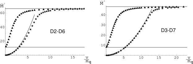
Figure 4: In this figure we plot the numerical masses for the first level as a function of the instanton size for both the full equation (with stars) and for the equation obtained in [63] (with solid triangles). The quark mass $m_{q}$ is such that $g_{eff}(m_{q})=1$. The solid line corresponds to the WKB prediction (352) for small $v$. The plot on the left (right) corresponds to the D2-D6 (D3-D7) intersection.

It turns out that the mass levels for small $v$ are nicely represented analytically by means of the WKB approximation for the Schrödinger problem (340). The WKB method has been very successful [118, 119] in the calculation of the glueball mass spectra in the gauge/gravity correspondence and also provides rather reliable predictions for the mass levels of the mesons [52]. The WKB quantization rule is

$$\bigg{(}n+{1\over 2}\bigg{)}\pi=\int_{z_{1}}^{z_{2}}dz\,\sqrt{-V(z)}\quad n\geq 0\,,$$ (345)

where $n\in Z$ and $z_{1}$ and $z_{2}$ are the turning points of the potential ($V(z_{1})=\break V(z_{2})=0$). Following straightforwardly the steps of [119] and [52], we obtain the following expression for the WKB values of $\bar{M}$:

$$\bar{M}_{\rm WKB}^{2}={\pi^{2}\over\zeta^{2}}\,(n+1)\bigg{(}n+3+{2\over 5-p}\bigg{)}\,,$$ (346)

where $\zeta$ is the following integral:

$$\zeta=\int_{0}^{+\infty}d\varrho\sqrt{{1\over(1+\varrho^{2})^{{7-p\over 2}}}+{c_{p}(v,m_{q})\over\Big{[}\big{(}{v\over m_{q}}\big{)}^{2}+\varrho^{2}\Big{]}^{4}}}\,.$$ (347)

Let us evaluate analytically $\zeta$ when $v$ is small. First of all, as can be easily checked, we notice that, when $v$ is small, the second term under the square root in (347) behaves as

$${1\over\Big{[}\big{(}{v\over m_{q}}\big{)}^{2}+\varrho^{2}\Big{]}^{2}}\approx{\pi\over 2}\bigg{(}{m_{q}\over v}\bigg{)}^{3}\delta(\varrho)\,,\quad{\rm as}\quad v\to 0\,.$$ (348)

Then, one can see that this term dominates the integral defining $\zeta$ around $\varrho\approx 0$ and, for small $v$, one can approximate $\zeta$ as

$$\zeta\approx{\sqrt{c_{p}(v,m_{q})}\over 2}\int_{-\epsilon}^{\epsilon}{d\varrho\over\Big{[}\big{(}{v\over m_{q}}\big{)}^{2}+\varrho^{2}\Big{]}^{2}}+\int_{0}^{+\infty}{d\varrho\over(1+\varrho^{2})^{{7-p\over 4}}}\,,$$ (349)

where $\epsilon$ is a small positive number and we have used the fact that the function in (347) is an even function of $\varrho$. Using (348), one can evaluate $\zeta$ as

$$\zeta\approx{\pi\over 4}\bigg{(}{m_{q}\over v}\bigg{)}^{3}\sqrt{c_{p}(v,m_{q})}+{\sqrt{\pi}\over 2}\,{\Gamma\big{(}{5-p\over 4}\big{)}\over\Gamma\big{(}{7-p\over 4}\big{)}}\,.$$ (350)

Clearly, for $v\to 0$, we can neglect the last term in (350). Using the expression of $c_{p}(v,m_{q})$ (Eq. (154)), we arrive at

$$\zeta\approx{\sqrt{3}\cdot 2^{{p-4\over 2}}\pi^{{p+5\over 4}}\over\sqrt{\Gamma\big{(}{7-p\over 2}\big{)}}}\,{m_{q}\over g_{\rm eff}(m_{q})v}\,,$$ (351)

and plugging this result in (346), we get the WKB mass of the ground state ($n=0$) for small $v$:

$$\bar{M}_{\rm WKB}^{2}\approx{(17-3p)\Gamma\big{(}{5-p\over 2}\big{)}\over 3\cdot 2^{p-3}\pi^{{p+1\over 2}}}\bigg{(}{g_{\rm eff}(m_{q})v\over m_{q}}\bigg{)}^{2}\,.$$ (352)

Thus, we predict that $\bar{M}^{2}$ is a quadratic function of $v/m_{q}$ with the particular coefficient given on the r.h.s. of (352). In Fig. 4 we have represented by a solid line the value of $\bar{M}$ obtained from Eq. (352). We notice that, for small $v$, this equation nicely fits the values obtained by the numerical calculation.

References

- [1] J. M. Maldacena, “The large limit of superconformal field theories and supergravity” Adv. Theor. Math. Phys. 2 (1998) 231, hep-th/9711200.
- [2] O. Aharony, S. Gubser, J. Maldacena, H. Ooguri and Y. Oz, “Large field theories, string theory and gravity”, Phys. Rept. 323 (2000) 183, hep-th/9905111.
- [3] L. Susskind and E. Witten, “The holographic bound in anti-de Sitter space,” arXiv:hep-th/9805114.
- [4] E. Witten, “Anti-de Sitter space and holography,” Adv. Theor. Math. Phys. 2 (1998) 253 arXiv:hep-th/9802150.
- [5] S. S. Gubser, I. R. Klebanov and A. M. Polyakov, “Gauge theory correlators from non-critical string theory,” Phys. Lett. B 428, 105 (1998) arXiv:hep-th/9802109.
- [6] S. Benvenuti, S. Franco, A. Hanany, D. Martelli and J. Sparks, “An infinite family of superconformal quiver gauge theories with Sasaki-Einstein duals,” J. High Energy Phys. 0506 (2005) 064 arXiv:hep-th/0411264.
- [7] S. Benvenuti and M. Kruczenski, “From Sasaki-Einstein spaces to quivers via BPS geodesics: L(p,q—r),” J. High Energy Phys. 0604 (2006) 033 arXiv:hep-th/0505206.
- [8] S. Franco, A. Hanany, D. Martelli, J. Sparks, D. Vegh and B. Wecht, “Gauge theories from toric geometry and brane tilings,” J. High Energy Phys. 0601 (2006) 128 arXiv:hep-th/0505211.
- [9] A. Butti, D. Forcella and A. Zaffaroni, “The dual superconformal theory for L(p,q,r) manifolds,” J. High Energy Phys. 0509 (2005) 018 arXiv:hep-th/0505220.
- [10] I. R. Klebanov and E. Witten, “ Superconformal field theory on threebranes at a Calabi-Yau singularity, Nucl. Phys. B 536, 199 (1998), arXiv:hep-th/9905104.
- [11] I. R. Klebanov and A. Murugan, “Gauge / gravity duality and warped resolved conifold,” J. High Energy Phys. 0703 (2007) 042 arXiv:hep-th/0701064.
- [12] I. R. Klebanov and M. J. Strassler, “Supergravity and a confining gauge theory: Duality cascades and chiSB-resolution of naked singularities,” J. High Energy Phys. 0008 (2000) 052 arXiv:hep-th/0007191.
- [13] H. J. Boonstra, K. Skenderis and P. K. Townsend, “The domain wall/QFT correspondence,” J. High Energy Phys. 9901 (1999) 003 arXiv:hep-th/9807137.
- [14] N. Itzhaki, J. M. Maldacena, J. Sonnenschein and S. Yankielowicz, “Supergravity and the large N limit of theories with sixteen supercharges,” Phys. Rev. D 58 (1998) 046004 arXiv:hep-th/9802042.
- [15] M. Bertolini, P. Di Vecchia, M. Frau, A. Lerda, R. Marotta and I. Pesando, “Fractional D-branes and their gauge duals,” J. High Energy Phys. 0102 (2001) 014 arXiv:hep-th/0011077.
- [16] M. Bertolini, P. Di Vecchia, M. Frau, A. Lerda and R. Marotta, “N = 2 gauge theories on systems of fractional D3/D7 branes,” Nucl. Phys. B 621 (2002) 157 arXiv:hep-th/0107057.
- [17] M. Grana and J. Polchinski, “Gauge / gravity duals with holomorphic dilaton,” Phys. Rev. D 65 (2002) 126005 arXiv:hep-th/0106014.
- [18] A. Karch and L. Randall, “Locally localized gravity”, J. High Energy Phys. 0105 (2001) 008, hep-th/0011156.
- [19] “Open and closed string interpretation of SUSY CFT’s on branes with boundaries”, J. High Energy Phys. 0106 (2001) 063, hep-th/0105132.
- [20] A. Karch and E. Katz, “Adding flavor to AdS/CFT”, J. High Energy Phys. 0206 (2002) 043, hep-th/0205236.
- [21] A. Karch, E. Katz and N. Weiner, “Hadron masses and screening from AdS Wilson loops”, Phys. Rev. Lett. 90 (2003) 091601, hep-th/0211107.
- [22] M. Kruczenski, D. Mateos, R. Myers and D. Winters, “Meson spectroscopy in AdS/CFT with flavour”, J. High Energy Phys. 0307 (2003) 049, hep-th/0304032
- [23] T. Sakai and J. Sonnenschein, “Probing flavored mesons of confining gauge theories by supergravity”, J. High Energy Phys. 0309 (2003) 047, hep-th/0305049.
- [24] J. Babington, J. Erdmenger, N. Evans, Z. Guralnik and I. Kirsch, “Chiral symmetry breaking and pions in non-supersymmetric gauge/gravity duals”, Phys. Rev. D69 (2004) 066007, hep-th/0306018.
- [25] R. Apreda, J. Erdmenger and N. Evans, “Scalar effective potential for D7-brane probes which break chiral symmetry”, hep-th/0509219.
- [26] R. Apreda, J. Erdmenger, N. Evans, J. Grosse and Z. Guralnik, “Instantons on D7 brane probes and AdS/CFT with flavour”, hep-th/0601130.
- [27] M. Kruczenski, D. Mateos, R. Myers and D. Winters, ‘Towards a holographic dual of large- QCD”, J. High Energy Phys. 0405 (2004) 041, hep-th/0311270.
- [28] J. L. F. Barbon, C. Hoyos, D. Mateos and R. C. Myers, “The holographic life of the eta’”, J. High Energy Phys. 0410 (2004) 029, hep-th/0404260.
- [29] A. Armoni, “Witten-Veneziano from Green-Schwarz”, J. High Energy Phys. 0406, 019 (2004), hep-th/0404248.
- [30] J. L. Hovdebo, M. Kruczenski, D. Mateos, R. C. Myers and D. J. Winters, “Holographic mesons: Adding flavor to the AdS/CFT duality,” Int. J. Mod. Phys. A 20 (2005) 3428.
- [31] P. Ouyang, “Holomorphic D7-branes and flavored N=1 gauge dynamics”, Nucl. Phys. B699 (2004) 207, hep-th/0311084.
- [32] T. S. Levi and P. Ouyang, “Mesons and flavor on the conifold”, hep-th/0506021.
- [33] X.-J. Wang and S. Hu, “Intersecting branes and adding flavors to the Maldacena-Núñez background”, J. High Energy Phys. 0309 (2003) 017 hep-th/0307218.
- [34] C. Núñez, A. Paredes and A. V. Ramallo, “Flavoring the gravity dual of Yang-Mills with probes”, J. High Energy Phys. 0312 (2003) 024, hep-th/0311201.
- [35] S. Hong, S. Yoon, M. J. Strassler, “Quarkonium from the fifth dimension”, J. High Energy Phys. 0404 (2004) 046, hep-th/0312071.
- [36] N. Evans, J. P. Shock, “Chiral dynamics from AdS space”, Phys. Rev. D70 (2004) 046002,hep-th/0403279.
- [37] N. Evans, J. P. Shock and T. Waterson, “D7 brane embeddings and chiral symmetry breaking”, J. High Energy Phys. 0503 (2005) 005, hep-th/0502091.
- [38] J. P. Shock, “Canonical coordinates and meson spectra for scalar deformed SYM from the AdS/CFT correspondence”, hep-th/0601025.
- [39] K. Ghoroku, M. Yahiro, “Chiral symmetry breaking driven by the dilaton”, Phys. Lett. B604 (2004) 235, hep-th/0408040.
- [40] “Holographic models for mesons at finite temperature”, hep-ph/0512289.
- [41] K. Ghoroku, T. Sakaguchi, N. Uekusa and M. Yahiro, “Flavor quark at high temperature from a holographic model”, Phys. Rev. D71 (2005) 106002, hep-th/0502088.
- [42] I. Brevik, K. Ghoroku and A. Nakamura, “Meson mass and confinement force driven by the dilaton”, hep-th/0505057.
- [43] K. Peeters, J. Sonnenschein and M. Zamaklar, “Holographic melting and related properties of mesons in a quark gluon plasma”, Phys. Rev. D 74,106008 (2006), hep-th/0606195.
- [44] S. Kobayashi, D. Mateos, S. Matsuura, R. C. Myers and R. M. Thomson, “Holographic phase transitions at finite baryon density”, J. High Energy Phys. 0702, 016 (2007), hep-th/0611099.
- [45] C. Hoyos, K. Landsteiner and S. Montero, “Holographic meson melting”, hep-th/0612169.
- [46] D. Mateos, R. C. Myers and R. M. Thomson, “Thermodynamics of the brane”, hep-th/0701132.
- [47] D. Arean, D. Crooks and A. V. Ramallo, “Supersymmetric probes on the conifold”, J. High Energy Phys. 0411 (2004) 035, hep-th/0408210.
- [48] S. Kuperstein, “Meson spectroscopy from holomorphic probes on the warped deformed conifold”, J. High Energy Phys. 0503 (2005) 014, hep-th/0411097.
- [49] T. Sakai and S. Sugimoto, “Low energy hadron physics in holographic QCD”, Prog. Theor. Phys. 113 (2005) 843, hep-th/0412141.
- [50] “More on a holographic dual of QCD”, Prog. Theor. Phys. 114 (2006) 1083, hep-th/0507073;
- [51] D. Arean, A. Paredes and A. V. Ramallo, “Adding flavor to the gravity dual of non-commutative gauge theories,” J. High Energy Phys. 0508 (2005) 017, hep-th/0505181.
- [52] D. Arean and A. V. Ramallo, “Open string modes at brane intersections”, J. High Energy Phys. 0604 (2006) 037, hep-th/0602174.
- [53] R.C.Myers, R.M.Thompson, ”Holographic mesons in various dimensions”, J. High Energy Phys.0609 (2006) 066, hep-th/0605017.
- [54] R. Apreda, J. Erdmenger, D. Lust and C. Sieg, “Adding flavour to the Polchinski-Strassler background”, J. High Energy Phys. 0701, 079 (2007), hep-th/0610276.
- [55] A. V. Ramallo, “Adding open string modes to the gauge/gravity correspondence”, Mod. Phys. Lett. A21 (2006) 1, hep-th/0605261.
- [56] R. Casero, C. Nunez and A. Paredes, “ Towards the string dual of N = 1 SQCD-like theories,” Phys. Rev. D 73, 086005 (2006), hep-th/0602027.
- [57] A. Paredes, “ On unquenched N = 2 holographic flavor,” J. High Energy Phys. 0612 (2006) 032, hep-th/0610270.
- [58] R. Casero and A. Paredes, “A note on the string dual of N = 1 SQCD-like theories,” hep-th/0701059.
- [59] F. Benini, F. Canoura, S. Cremonesi, C. Núñez and A. V. Ramallo, “Unquenched flavors in the Klebanov-Witten model”, J. High Energy Phys. 0702 (2007) 090, hep-th/0612118.
- [60] F. Benini, “A chiral cascade via backreacting D7-branes with flux,” arXiv:0710.0374 [hep-th].
- [61] R. Casero, C. Nunez and A. Paredes, “Elaborations on the String Dual to N=1 SQCD,” arXiv:0709.3421 [hep-th].
- [62] F. Benini, F. Canoura, S. Cremonesi, C. Nunez and A. V. Ramallo, “Backreacting Flavors in the Klebanov-Strassler Background,” arXiv:0706.1238 [hep-th].
- [63] J.Erdmenger, J. Grosse, Z. Guralnick, ”Spectral flow on the Higgs branch and duality”, J. High Energy Phys. 0506 (2005) 052, hep-th/0502224.
- [64] Z. Guralnik, S. Kovacs and B. Kulik, “Holography and the Higgs branch of N = 2 SYM theories”, J. High Energy Phys. 0503, 063 (2005), hep-th/0405127.
- [65] D. Arean, A. V. Ramallo and D. Rodriguez-Gomez, “Holographic flavor on the Higgs branch,” J. High Energy Phys. 0705 (2007) 044 arXiv:hep-th/0703094.
- [66] A. Giveon and D. Kutasov, “Brane dynamics and gauge theory,” Rev. Mod. Phys. 71, 983 (1999) hep-th/9802067.
- [67] O. Aharony, “A note on the holographic interpretation of string theory backgrounds with varying flux,” J. High Energy Phys. 0103 (2001) 012 arXiv:hep-th/0101013.
- [68] R. C. Myers, “Dielectric branes”, J. High Energy Phys. 9912 (1999) 022, hep-th/9910053
- [69] O. DeWolfe, D. Z. Freedman and H. Ooguri, “Holography and defect conformal field theories”, Phys. Rev. D66 (2002) 025009, hep-th/0111135.
- [70] J. Erdmenger, Z. Guralnik and I. Kirsch, “Four-dimensional superconformal theories with interacting boundaries or defects”, Phys. Rev. D66 (2002) 025020, hep-th/0203020.
- [71] D.Arean, A.V.Ramallo, D.Rodriguez-Gomez, ”Mesons and Higgs branch in defect theories”, Phys. Lett. B641 (2006) 393, hep-th/0609010.
- [72] K.Skenderis, M.Taylor, ”Branes in and -wave spacetimes”, J. High Energy Phys. 0206 (2002) 025, hep-th/0204054.
- [73] N.Constable, Z.Guralnik, J.Erdmenger, I.Kirch, ”Intersecting D3-branes and holography”, Phys. Rev. D68 (2003) 106007, hep-th/0211222.
- [74] J. Erdmenger, Z. Guralnik, R. Helling and I. Kirsch, “A world-volume perspective on the recombination of intersecting branes,” J. High Energy Phys. 0404 (2004) 064, hep-th/0309043.
- [75] I. Kirsch, “Generalizations of the AdS/CFT correspondence,” Fortsch. Phys. 52 (2004) 727, hep-th/0406274.
- [76] I. R. Klebanov and E. Witten, “AdS/CFT correspondence and symmetry breaking,” Nucl. Phys. B 556 (1999) 89 arXiv:hep-th/9905104.
- [77] I. R. Klebanov, “World-volume approach to absorption by non-dilatonic branes,” Nucl. Phys. B 496 (1997) 231 arXiv:hep-th/9702076.
- [78] S. S. Gubser, I. R. Klebanov and A. A. Tseytlin, “String theory and classical absorption by three-branes,” Nucl. Phys. B 499 (1997) 217 arXiv:hep-th/9703040.
-
[79]
S. S. Gubser and I. R. Klebanov,
“Absorption by branes and Schwinger terms in the world volume theory,”
Phys. Lett. B 413 (1997) 41
arXiv:hep-th/970800
- [80] E. D’Hoker and D. Z. Freedman, “Supersymmetric gauge theories and the AdS/CFT correspondence,” arXiv:hep-th/0201253.
- [81] K. Skenderis, “Lecture notes on holographic renormalization,” Class. Quant. Grav. 19 (2002) 5849 arXiv:hep-th/0209067.
- [82] K. Behrndt, E. Bergshoeff and B. Janssen, “Intersecting –Branes in Ten and Six Dimensions,” Phys. Rev. D55 (1997) arXiv:hep-th/9604168.
- [83] E. Bergshoeff, M. de Roo, E. Eyras, B. Janssen and J. P. van der Schaar, “Multiple intersections of D-branes and M-branes,” Nucl. Phys. B 494 (1997) 119 arXiv:hep-th/9612095.
- [84] M.R.Douglas, ”Branes within branes”, hep-th/9512077.
- [85] M.R.Douglas, ”Gauge Fields and D-branes”, J. Geom. Phys.28, 255 (1998), hep-th/9604198.
- [86] E.Witten, ”Sigma models and the construction of instantons”, J. Geom. Phys.15, 215 (1995), hep-th/9410052.
- [87] D. Tong, “TASI lectures on solitons: instantons, monopoles, vortices and kinks”, hep-th/0509216.
-
[88]
N. Dorey, T. J. Hollowood, V. V. Khoze and M. P. Mattis,
“The calculus of many instantons,”
Phys. Rept. 371 (2002) 231
arXiv:hep-th/0206063.
- [89] M. R. Douglas and N. A. Nekrasov, “Noncommutative field theory,” Rev. Mod. Phys. 73 (2001) 977 arXiv:hep-th/0106048.
- [90] N. Seiberg and E. Witten, “String theory and non-commutative geometry”, J. High Energy Phys. 9909 (1999) 032, hep-th/9908142.
- [91] D.Rodriguez-Gomez, jhep vol0601, 079 (2006), hep-th/0509228.
- [92] B. Janssen, Y. Lozano and D. Rodriguez-Gomez, “The baryon vertex with magnetic flux,” jhep 0611 (2006) 082, arXiv:hep-th/0606264.
- [93] A. Hanany and E. Witten, “Type IIB superstrings, BPS monopoles, and three-dimensional gauge dynamics,” Nucl. Phys. B 492 (1997) 152 arXiv:hep-th/9611230.
- [94] C. Bachas, M. Douglas and C. Schweigert, “Flux stabilization of D-branes”, J. High Energy Phys. 0005 (2000) 048, hep-th/0003037.
- [95] W.Nahm in N. S. Craigie, P. Goddard and W. Nahm, “Monopoles In Quantum Field Theory. Proceedings, Monopole Meeting, Trieste, Italy, December 11-15, 1981,”
- [96] C. G. . Callan and J. M. Maldacena, “Brane dynamics from the Born-Infeld action,” Nucl. Phys. B 513 (1998) 198 arXiv:hep-th/9708147.
- [97] P.Pasti, D.Sorokin, M.Tonin, ”Covariant action for a ”d=11” five-brane with the chiral field”, Phys. Lett. B398 (1997) 41, hep-th/9701037.
- [98] I. Bandos, K. Lechner, A. Nurmagambetov, P. Pasti, D. Sorokin and M. Tonin, Phys. Rev. Lett. 78 (1997) 4332, hep-th/9701149.
- [99] D. Sorokin, “On some features of the M5-brane”, hep-th/9807050.
- [100] J. M. Camino, A. Paredes and A. V. Ramallo, “Stable wrapped branes,” J. High Energy Phys. 0105 (2001) 011, hep-th/0104082.
- [101] F. Canoura, J. D. Edelstein, L. A. P. Zayas, A. V. Ramallo and D. Vaman, “Supersymmetric branes on AdS(5) x Y**(p,q) and their field theory duals,” J. High Energy Phys. 0603 (2006) 101, hep-th/0512087.
- [102] F. Canoura, J. D. Edelstein and A. V. Ramallo, “D-brane probes on L(a,b,c) superconformal field theories,” J. High Energy Phys. 0609 (2006) 038 arXiv:hep-th/0605260.
- [103] J. M. Maldacena and C. Nunez, “Towards the large N limit of pure N = 1 super Yang Mills,” Phys. Rev. Lett. 86 (2001) 588 arXiv:hep-th/0008001.
- [104] A. H. Chamseddine and M. S. Volkov, “Non-Abelian BPS monopoles in N = 4 gauged supergravity,” Phys. Rev. Lett. 79 (1997) 3343 arXiv:hep-th/9707176.
- [105] D. Arean, A. Paredes and A. V. Ramallo, “Adding flavor to the gravity dual of non-commutative gauge theories,” J. High Energy Phys. 0508 (2005) 017 arXiv:hep-th/0505181.
- [106] D. Mateos, String theory and quantum chromodynamics, arXiv:0709.1523.
- [107] D. Mateos, R. C. Myers and R. M. Thomson, “Holographic phase transitions with fundamental matter,” Phys. Rev. Lett. 97 (2006) 091601 arXiv:hep-th/0605046.
- [108] T. Albash, V. G. Filev, C. V. Johnson and A. Kundu, “A topology-changing phase transition and the dynamics of flavour,” arXiv:hep-th/0605088
- [109] V. G. Filev, C. V. Johnson, R. C. Rashkov and K. S. Viswanathan, “Flavoured large N gauge theory in an external magnetic field,” JHEP 0710 (2007) 019 [arXiv:hep-th/0701001].
- [110] V. G. Filev, “Criticality, Scaling and Chiral Symmetry Breaking in External Magnetic Field,” arXiv:0706.3811 [hep-th].
- [111] T. Albash, V. G. Filev, C. V. Johnson and A. Kundu, “Finite Temperature Large N Gauge Theory with Quarks in an External Magnetic Field,” arXiv:0709.1547 [hep-th].
- [112] T. Albash, V. G. Filev, C. V. Johnson and A. Kundu, “Quarks in an External Electric Field in Finite Temperature Large N Gauge Theory,” arXiv:0709.1554 [hep-th].
- [113] A. O. Starinets, “Quasinormal modes of near extremal black branes,” Phys. Rev. D 66 (2002) 124013 arXiv:hep-th/0207133.
- [114] P. Kovtun, D. T. Son and A. O. Starinets, “Viscosity in strongly interacting quantum field theories from black hole physics,” Phys. Rev. Lett. 94 (2005) 111601 arXiv:hep-th/0405231.
- [115] C. P. Herzog, A. Karch, P. Kovtun, C. Kozcaz and L. G. Yaffe, “Energy loss of a heavy quark moving through N = 4 supersymmetric Yang-Mills plasma,” J. High Energy Phys. 0607 (2006) 013 arXiv:hep-th/0605158.
- [116] S. S. Gubser, “Drag force in AdS/CFT,” Phys. Rev. D 74 (2006) 126005 arXiv:hep-th/0605182.
- [117] H. Liu, K. Rajagopal and U. A. Wiedemann, “Calculating the jet quenching parameter from AdS/CFT,” Phys. Rev. Lett. 97 (2006) 182301 arXiv:hep-ph/0605178.
- [118] J. A. Minahan, “Glueball mass spectra and other issues for supergravity duals of QCD models”, J. High Energy Phys. 9901 (1999) 020, hep-th/9811156.
- [119] J. G. Russo and K. Sfetsos, “Rotating D3-branes and QCD in three dimensions”, Adv. Theor. Math. Phys. 3(1999) 131, hep-th/9901056.
- [120] E. Witten, “Bound states of strings and p-branes,” Nucl. Phys. B 460 (1996) 335 arXiv:hep-th/9510135.
- [121] See B. Janssen, Y. Lozano and D. Rodriguez-Gomez, “Giant gravitons as fuzzy manifolds,” arXiv:hep-th/0412037 and references therein.