Abstract

We present a procedure to study the switching and the stability of an array of magnetic nanoparticles in the dynamical regime. The procedure leads to the criterion of multi-switching stability to be satisfied in order to have stable switching. The criterion is used to compare various magnetic-field-induced switching schemes, either present in the literature or suggested in the present work. In particular, we perform micromagnetic simulations to study the magnetization trajectories and the stability of the magnetization after switching for nanoparticles of elliptical shape. We evaluate the stability of the switching as a function of the thickness of the particles and the rise and fall times of the magnetic pulses, both at zero and room temperature. Furthermore, we investigate the role of the dipolar interaction and its influence on the various switching schemes. We find that the criterion of multi-switching stability can be satisfied at room temperature and in the presence of dipolar interactions for pulses shaped according to CMOS specifications, for switching rates in the GHz regime.

I. Introduction

The magnetization reversal and the state stability of magnetic particles are key issues in magnetic technology applications. In particles with uniaxial anisotropy the direction of the magnetization can be changed by applying a field pulse either parallel or perpendicular to the magnetic easy axis. The reversal times, which depend on the speed and the direction of the applied field, vary from many nanoseconds (damping switching) to hundreds of picoseconds (ballistic precessional switching)[1, 2, 3, 4]. The stability of the particle’s magnetization configuration after switching depends on several factors, such as the temperature of the system, the size of the particle and the shape of the applied fields. Furthermore, in arrays of magnetic particles the dipolar interaction and the not perfectly equal shape of the particles shrinks the switching margin used to switch a selected particle without affecting other ones, the so-called half selected particles[5].

In this work we present a procedure to study the stability of an array of magnetic particles for magnetic-field-induced switching schemes: First we analyze the stability of the half-selected particles with respect to a chosen switching scheme; second, we investigate the precessional switching of the particle of interest (fully-selected particle)(section II-B); third, we check the stability of the state obtained after switching as well as the possibility of stable successive switchings. Such a procedure leads us to define the criterion of multi-switching stability to be satisfied in order to have stable and repeatable switching (sec. II-C). In the second part of the paper we extend the investigation by considering the array as a function of various parameters such as the thickness of the particles, the duration of the pulse, the temperature (sec. III) and the strength of the dipolar interaction (sec. IV).

II. Magnetization dynamics

A. Addressing schemes

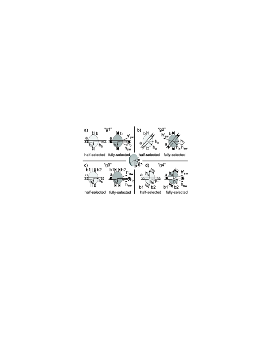
Figure 1: Addressing schemes. ”g1”: Classical cross-wire geometry. ”g2”: Geometry after Ref [7]. ”g3”: Classical geometry with improved stability. ”g4”: Tilted geometry with improved stability. For each geometry we show the half-selected particle and the fully-selected particle. To the half (fully)-selected particle are applied either (both) the magnetic field $h_{a}$ or (and) the magnetic field $h_{b}$.

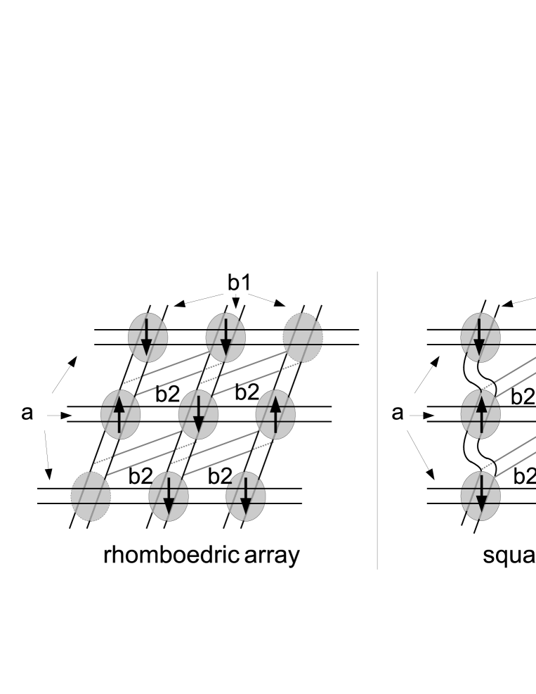
Figure 8: Array geometries. Left: rhomboedric array. Right: square array. The wiring is similar in proximity of the magnetic particles. Only the cylinders with arrows are used for the calculation.

In Fig. 1a we draw the classical cross-wire geometry used to write a magnetic cell by means of magnetic fields[5]. The field h${{}_{\textbf{sw}}}$ (h${}^{\prime}{{}_{\textbf{sw}}}$) is used to switch the magnetization from up to down (down to up) and it is given by the sum of the fields h${{}_{\textbf{a}}}$ and h${{}_{\textbf{b}}}$ produced by the current flow in line a (or ”bit line”) and line b (or ”word line”), respectively. Such a scheme involves a bipolar current flow in line a necessary to obtain the two opposite directions of h${{}_{\textbf{a}}}$. In general, in order to guarantee the stability of the half-selected particles, the field components $h_{a}$ and $h_{b}$ must not exceed the values specified by the border of the corresponding magnetic astroid. The operation margin associated to the above mentioned classical geometry (called ”g1”, from here on) does not guarantee sufficient stability in the presence of dipolar interaction and thermal fluctuations[5]. Because of that a much more stable switching scheme has been developed[6], which led to the first commercial 4-Mb magnetic-RAM device. As an alternative, to enlarge the operation margin one can reduce the values of the fields $h_{a}$ and/or $h_{b}$ without changing the field h${{}_{\textbf{sw}}}$. Vectorially this is obtained by varying the angle between the line-a and line-b[7], see Fig. 1b. In such a geometry, (labelled ”g2”) the field h${}^{\prime}{{}_{\textbf{sw}}}$ is obtained by inverting the current flow direction in both lines, a and b. Thus, the addressing scheme is of ”double-dipolar” type. Another way to enlarge the operation margin is to add a third set of lines to the wiring geometry, thus reducing the magnetic field acting on the half-selected particles. For example, one can divide line-b in two sub-lines ”$b_{1}$” and ”$b_{2}$”, see Fig. 1c-d, each one producing a magnetic field h${{}_{\textbf{b}}}$. Lines ”$b_{1}$” and ”$b_{2}$” can be built in stack separated by a insolating layer. These lines contribute to the switching process of a fully-selected particle with the total magnetic field 2h${{}_{\textbf{b}}}$. Due to the wiring geometry, see Fig. 8, a half-selected particle is subjected only to the field h${{}_{\textbf{b}}}$, which enhances its stability. In the geometry of Fig. 1c (”g3”) lines ”$b_{1}$” and ”$b_{2}$” are parallel to the magnetic easy axis of the particle, as for the geometry ”g1”. The switching scheme in the two cases is similar. In the geometry of Fig. 1d (”g4”) lines ”$b_{1}$” and ”$b_{2}$” are tilted by the angle $\beta$ with respect to the magnetic easy axis. The magnetic fields h${{}_{\textbf{a}}}$ and h${{}_{\textbf{b}}}$ are applied to the half-selected particles. In the fully-selected particle the magnetization m switches by application of the magnetic field h${{}_{\textbf{sw}}}$ or h${}^{\prime}{{}_{\textbf{sw}}}$, with h${{}_{\textbf{sw}}}$=2 h${{}_{\textbf{b}}}$. The fields ${h_{a}}$ and ${h_{sw}}$ are related by the expression ${h_{a}}$=2 $h_{sw}$ sin $\beta$ so that h${{}_{\textbf{sw}}}$ and h${}^{\prime}{{}_{\textbf{sw}}}$ are equal in module but symmetrically oriented with respect to the minor axis of the ellipse. In contradistinction to the examples in Figs. 1a-c, this addressing scheme allows easy switching by the use of unipolar magnetic field pulses, as will be detailed later.

B. Stability regions, switching trajectories and pulse synchronism

In the following section we study the switching properties and the stability of an isolated elliptical cylinder. To be explicit, the major and the minor semi-axis of the cylinder are 50 nm and 40 nm long, respectively. The hight is 1 nm. The direction of the average magnetization is given by the latitude $\theta$, measured from the plane of the particle, and the azimuthal angle $\phi$, measured from the easy axis of the particle (Fig. 1). The material is iron with cubic anisotropy constant k=1.5$\times 10^{4}$ J/m³[8], exchange stiffness constant A=2.1$\times 10^{-11}$ J/m and saturation magnetization M_s=1.714$\times 10^{6}$ A/m³[9]. For this choice of the geometry and the magnetic constants the total energy is dominated by the stray field energy, being more than one order of magnitude larger than the exchange energy and the anisotropy energy. Thus, the system has two minima: one located at ($\theta=0^{\circ}$, $\phi=0^{\circ}$), the ”down” state or bit ”0”, the other at ($\theta=0^{\circ}$, $\phi=180^{\circ}$), the ”up” state or bit ”1”. Such an example is representative of any bi-stable system for which the energy of the particle is dominated by its shape.

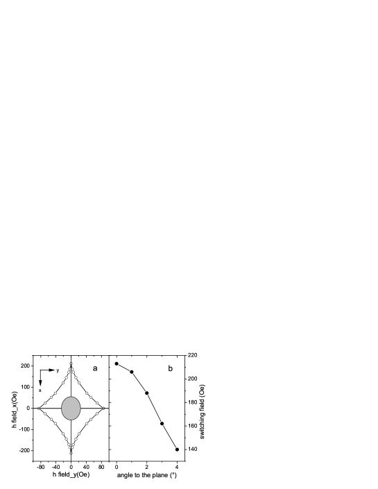
Figure 2: a: Dynamical astroid. The diagram is obtained for an elliptical cylinder with semi-axis of 50 nm and 40 nm, hight 1 nm. The field pulse is a step function with 200 ps rise-time. The damping factor is $\alpha$=0.02. b: Switching field vs. angle to the plane $\theta$.

We perform micromagnetic simulations[9] in order to study the magnetization trajectories and the stability of the magnetic states obtained after application of an external magnetic field pulse. The Landau-Lifshitz-Gilbert (LLG) equation of motion is solved in the dynamic regime by using a value of the damping factor $\alpha$= 0.02. The simulation volume is divided in unit cells of parallelepiped shape with an edge of 2 nm in the plane and 1 nm in thickness. In Fig. 2a we show the dynamical astroid[1] obtained for a pulse with a rise time of 200 ps. By applying a magnetic field antiparallel to the magnetization direction we find that the field necessary to overcome the barrier between the two minima is 213 Oe. It is worth to note that often in the literature the analysis of the switching behavior of a magnetic particle is 2-dimensional, while the complete scenario is given by means of a 3D analysis[10]. To understand this fact, in Fig. 2b we plot the magnetic field necessary to switch the magnetization as a function of the latitude $\theta$. For the selected $\alpha$= 0.02 the switching field is reduced dramatically by 73 Oe when increasing the latitude to only 4^∘. The corresponding reduction in the damping regime (i.e. $\alpha$= 1) is 8 Oe. This difference is due to the differing amplitudes of the damping oscillations, viz. to the torque produced by the applied field on the average magnetization. This result shows that a 3D analysis is fundamental to study the switching and the stability of magnetic nanoparticles, in particular in the dynamical regime.

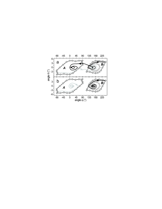
Figure 4: Criterion of multi-switching stability. The regions A and B contain the coordinates for which the magnetization is stable under the action of one single field, namely h${{}_{\textbf{a}}}$ or h${{}_{\textbf{b}}}$, respectively. The regions enclosed by the grey (open) dots are obtained for the [90^∘-$\beta$]-cross-wire (90^∘-cross-wire) geometry for h_sw=100 Oe (h_sw=80 Oe). Panel a: examples of switching (non perfectly synchronized pulses). The grey (black) line represents the trajectory of the average magnetization from the boundary of region A (B) into region B (A) by means of the field h${}^{\prime}{{}_{\textbf{sw}}}$ (h${{}_{\textbf{sw}}}$). Panel b: examples of no switching (non-perfectly synchronized pulses). The grey (black) line represents the trajectory from the boundary of region A (B) into the same region by means of the field h${{}_{\textbf{sw}}}$ (h${}^{\prime}{{}_{\textbf{sw}}}$).

In a 3D picture, in order to prove the stability of half selected particles we define a region in the plane ($\phi$ , $\theta$) where the magnetization is stable under the action of one single pulse. Let us consider a bi-stable system with energy minima in the ”down” state and in the ”up” state. If the magnetization is ”down” (”up”) it may switch because of field h${{}_{\textbf{a}}}$ (h${{}_{\textbf{b}}}$), according to the addressing scheme geometry ”g4”. Therefore we define two regions of stability in the plane ($\phi$ , $\theta$): region A, where the magnetization is stable under the application of the field h${{}_{\textbf{a}}}$ and region B, where the magnetization is stable under the application of the field h${{}_{\textbf{b}}}$ (see Fig. 4). The stability region A is obtained by applying a step function of module h_a= 68.4 Oe with 200 ps rise time (the value of h_a is related to h_sw= 100 Oe, using $\beta=20^{\circ}$). At $\theta=0^{\circ}$ the magnetic state is stable for $-69^{\circ}\leq\phi\leq 69^{\circ}$. At $\phi=0^{\circ}$ the magnetic state is stable for $-4.9^{\circ}\leq\theta\leq 4.9^{\circ}$. A similar analysis is done for the stability region B. This region is obtained by applying a step function of module h_b= 50 Oe with 200 ps rise time. At $\theta=0^{\circ}$ the magnetic state is stable for $131^{\circ}\leq\phi\leq 228^{\circ}$. At $\phi=180^{\circ}$ the magnetic state is stable for $-4^{\circ}\leq\theta\leq 4.9^{\circ}$. By analyzing the two stability regions we notice that, on the one hand, the stability interval is quite large if the average magnetization lies in- or almost in-plane; on the other hand, the stability interval is strongly reduced for $\theta\neq 0$. As a consequence only the particles with the magnetization close to the plane are stable. Note that in order to have stability in one region the magnetization has to relax from each border-point of the stability region into the minimum with a damping trajectory belonging to said region. In that case, a pulse applied at any time cannot lead to the instability of a half-selected particle. In Fig. 4 and in the following we plot stability regions obtained after a refinement procedure, which consists in reducing the stability regions until the relaxing trajectories fully belong to the respective regions.

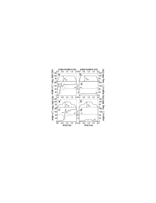
Figure 3: Switching of the magnetization. Panels a-b (a’-b’): shape of the magnetic field with synchronized (non-perfectly synchronized) pulses. Panels c-d/c’-d’: magnetization trajectories. Panel c-c’: The magnetization switches from ”down” to ”up” by application of the field h${}^{\prime}{{}_{\textbf{sw}}}$. Panel d-d’: The magnetization does not switch by application of the field h${{}_{\textbf{sw}}}$.

The study of the magnetization switching is done by using the pulses shown in Fig. 3. The shape of the pulse in Fig. 3a-b is ”trapezoidal”. This pulse is characterized by the four segments ($t_{p},t_{r},t_{pl},t_{f}$), $t_{p}$ being the duration of the pulse, $t_{r}$ the rise time, $t_{pl}$ the central plateau and $t_{f}$ the fall time. Each time is given in nanoseconds. For example, the pulse in Fig. 3a-b is characterized by (2, 0.2, 1.6, 0.2). The direction of the magnetic field is h${}^{\prime}{{}_{\textbf{sw}}}$ and h${{}_{\textbf{sw}}}$, respectively, with maximum module $h_{m}$=100 Oe. In Fig. 3 c-d we plot the response of the averaged magnetization to the field pulses. In both cases the initial state of the system is ”down”, while the final state is either ”up” or ”down”. By means of the field h${}^{\prime}{{}_{\textbf{sw}}}$ the magnetization rotates towards the ”up” state. The switching takes place in the first 380 ps by means of a half precession. After that, the magnetization shows damped oscillations in a transient energy minimum at ($\theta\approx 0^{\circ}$, $\phi\approx 154^{\circ}$). In the last 200 ps, the magnetization reaches the new minimum in absence of the applied field. By means of the field h${{}_{\textbf{sw}}}$ the averaged magnetization does not switch. In the first 200 ps the magnetization reaches a transient temporary minimum at ($\theta\approx 0^{\circ}$, $\phi\approx 24^{\circ}$). The initial minimum is established after pulse termination. For both, switching and no switching, the final states are stable to the application of successive single magnetic field pulses since the magnetization trajectories terminate inside the regions of stability. The same conclusion is valid for the transient energy minima. As a consequence, stable switching is possible also for shorter pulses. Note that since the shape of the particle is not an ellipsoid the magnetization does not rotate coherently. Rather, due to the small size of the particle the magnetization rotates quasi-uniformly.

The pulses used above to switch the magnetization are given by the vectorial sum of two sub-pulses h${{}_{\textbf{sw}}}$= 2h${{}_{\textbf{b}}}$ and h${}^{\prime}{{}_{\textbf{sw}}}$=h${{}_{\textbf{sw}}}$ +h${{}_{\textbf{a}}}$. Up to here we have considered the sub-pulses as synchronized. Experimentally such a condition is difficult to realize in a large array of magnetic particles[11]. In order to study the effect of the non-perfect synchronism of the sub-pulses we consider the ”double trapezoidal” pulse shown in Fig. 3 a’-b’. This pulse is characterized by five segments ($t_{p},t_{r},t_{pl1},t_{pl2},t_{f}$), $t_{p}$ being the duration of the pulse, $t_{r}$ the rise time from zero to the first plateau and from the first plateau to the central one, $t_{pl1}$ the first and the last plateaus, $t_{pl2}$ the central plateau, $t_{f}$ the fall time from the central to the last plateau and from the last plateau to zero. Therefore, the pulse in Fig. 3a’-b’ is characterized by (2, 0.2, 0,3, 0.6, 0.2). In Fig. 3 c’-d’ we plot the response of the average magnetization to such a field pulse. As above, in both cases the initial state of the system is ”down”. The effect of the non-perfect synchronism is evident by comparing Fig. 3 c’-d’ with Fig. 3 c-d. The main effect on the switching is the time shift from 380 ps to 850 ps in which the magnetization rotates towards the new energy minimum orientation (compare Figs. 3 c/c’). The non-perfect synchronism affects also the no-switching process. As shown in Fig. 3 d’, the direction of the magnetization follows the shape of the pulse. The maximum value of the angle $\phi$ is reached at $t\approx 0.7$ ns, with a shift of $\approx 0.5$ ns with respect to Fig. 3 d. For both, switching and no-switching, the final states are stable, as in the case of synchronized pulses. Since the effect of the non-perfect synchronism is to shift the switching time without affecting the stability of the final state, the time scale of the switching will depend directly on the experimentally achievable timing. The set of switching processes analyzed above is completed by the two symmetric switchings for which the magnetization is initially oriented in the ”up” direction. If the four switchings are successful, the following proposition is valid: whatever is the initial state, the field h${}^{\prime}{{}_{\textbf{sw}}}$ (h${{}_{\textbf{sw}}}$) causes the magnetic particle to end up in the ”up” (”down”) state. Such a property allows successive magnetization reversals without time delay since no knowledge of the magnetization direction is required, in contradistinction to toggle switching schemes [12].

C. Criterion of multi-switching stability

Until this point we have studied the response of a magnetic particle to a field pulse by considering the initial magnetization as being located in one of the energy minima of the system. In the following we extend the analysis to a magnetic particle with initial state represented by any of the points inside the stability regions A and B. As above we consider the switching and the no-switching processes. Each point in regions A and B is tested with regard to the field pulses h${}^{\prime}{{}_{\textbf{sw}}}$ and h${{}_{\textbf{sw}}}$. If all the magnetization trajectories converge inside the corresponding stability regions the system is considered stable to successive switchings. If these convergence conditions are satisfied, we say that the system satisfies the criterion of multi-switching stability. In Fig. 4a-b we plot some examples of switching and no-switching trajectories obtained with the magnetic pulse shown in Fig. 3a’-b’. The initial states of the magnetization are located at the border of the stability regions. After pulse application the magnetization settles inside regions A or B. Such a behavior is found for all the points located at the border of the stability regions, which is sufficient to prove the convergence of any initial state belonging to the stability regions. By means of such a procedure we find that the criterion of multi-switching stability is satisfied by using both, synchronized and non-perfectly synchronized pulses.

The analysis presented in this section, valid for the switching scheme ”g4”, can be extended to any other switching geometry. In sec. IV-B we present a comparison between the addressing schemes introduced in sec. II-A.

III. Temperature, thickness and pulse rise-time dependencies

In the former sections we have used the LLG equation of motion, which provides a zero-temperature description of the magnetization processes. A non-zero-temperature description is obtained by means of the stochastic LLG equation, based on Langevin-dynamics[13]. In this section we extends the former analysis to the room-temperature regime. Furthermore, we study the switching and the stability as a function of the thickness of the elliptical cylinder and the rise time of the magnetic field pulse.

In section II-B we have shown that for a cylinder with hight $t=1$ nm at zero temperature for a pulse with rise time $t_{r}$=200 ps the switching field is $h_{sw}=213$ Oe. In correspondence, at room-temperature ($300$ K) we find $h_{sw}=162$ Oe. This result is in accordance with the reduction of the coercivity with the temperature found in arrays of submicron elliptically patterned permalloy thin films[14]. In order to understand the reduction, in Fig. 5 we plot the time dependence of the azimuthal angle $\phi$ at zero and room temperature, respectively. The plot is obtained with the magnetization starting conditions $\theta=0^{\circ}$, $\phi=45^{\circ}$ in zero field. One observes that at zero temperature the first two oscillations take place within 400 ps, while at room temperature this happens within 710 ps. Therefore, the duration of the oscillations increases with temperature. Because long oscillations are associated to a long action of the torque between the magnetization and the applied field, in order to switch the magnetization at room temperature it is necessary to apply a smaller field than at zero temperature. For this same reason in Fig. 6 the regions of stability at zero temperature (dashed line) are larger than those at room temperature (full-dot line). The regions are calculated employing the switching scheme ”g4”, following the procedure of sec. II-B. Furthermore, since at room temperature the system is described in the framework of the Langevin dynamics, the stability of the regions against stochastic fluctuations is checked by considering each border point as stable only after three ”destabilization” attempts have led to the same convergence point. The analysis of the damped oscillations explains also the observed growth of the stability regions with increasing the rise time from $t_{r}$=75 ps (open-dot line) to $t_{r}$=200 ps (full-dot line). In fact, a pulse with short rise time exerts its influence already on the first magnetization oscillation, which is the most unstable because it has the largest amplitude.

After the calculation of the stability regions we now study the switching of the magnetization. We consider pulses with durations of 1 ns, 1.5 ns and 2 ns, with rise times of 75 ps and 200 ps at room temperature. The amplitude of the pulse is $h_{sw}=100$ Oe. Comparing the results for all the parameters, when switching from the ”down” stability region some of the trajectories do not terminate inside the ”up” stability region. Therefore the criterion of multi-switching stability is not satisfied. One way to satisfy the criterion is to choose a long enough pulse and fall time, so to allow the magnetization to relax inside the stability region. However, this method does not improve the intrinsic stability of the system, represented by the area of the stability region. In the presence of the dipolar interaction this area is even further reduced (see sec. IV) and thus the switching-stability criterion will not be satisfied, even for longer pulses. Another way to enlarge the stability region is to increase the thickness of the particle, which also causes an increase of the coercivity[15]. For an elliptical cylinder with the same size as used above and height t=2 nm, we obtain at zero temperature a switching field $h_{sw}=230$ Oe by using a pulse with rise time $t_{r}$=200 ps directed antiparallel to the magnetization direction and a damping factor $\alpha=0.02$. At room temperature we obtain $h_{sw}=207$ Oe. In Fig. 6 we plot the stability regions obtained at room temperature for $h_{sw}=130$ Oe. This amplitude is higher than the one used for $t=1$ nm ($h_{sw}=100$ Oe), which does not lead to stable-switching. The regions obtained for thickness $t=2$ nm are larger than those obtained for $t=1$ nm, especially much so for the regions around the ”up” state ($\phi=180^{\circ}$). As for the cylinder with $t=1$ nm, also for $t=2$ nm the regions obtained for $t_{r}=75$ ps (open-triangle line) are smaller than those obtained for $t_{r}=200$ ps (full-triangle line).

In the following we study the switching of the magnetization employing scheme ”g4” by applying the field $h_{sw}=130$ Oe to a cylinder with $t=2$ nm at room temperature. We consider two pulses characterized by (1.5, 0.2, 0.2, 0.3, 0.2) and (2, 0.2, 0.2, 0.8, 0.2). As explained in sec. II-B, this ”double trapezoidal” pulse shape takes into account the non-perfect synchronism between sub-pulses. We observe that all the trajectories starting from the border of the ”down” stability region terminate inside the ”up” stability region. It is important to evaluate under which switching conditions the final states lie in close proximity to each other in the plane ($\theta-\phi$). This evaluation is then an implicit measure of the stability of the system in the presence of the dipolar interaction since in that case the stability regions tend to shrink. In that sense we define the dispersion index $\overline{d}=\sum_{i=1}^{N}d_{i}/N$ as the average distance between the final magnetization states and their midpoint ($\overline{x},\overline{y},\overline{z}$), with $d_{i}=((\overline{x}-x_{i})^{2}+(\overline{y}-y_{i})^{2}+(\overline{z}-z_{i})^{2})^{1/2}$, $\overline{x}=\sum_{i=1}^{N}x_{i}/N$, $\overline{y}=\sum_{i=1}^{N}y_{i}/N$, $\overline{z}=\sum_{i=1}^{N}z_{i}/N$ and ($x_{i}$, $y_{i}$, $z_{i}$) the cartesian coordinate of the final state i. The dispersion index related to the two pulses with duration $t_{p}=1.5$ ns and $t_{p}=2$ ns are $\overline{d}=0.114$ and $\overline{d}=0.05$, respectively. The dispersion is smaller for the pulse with longer duration, see Fig. 7. Next we consider two pulses characterized by (1.5, 0.075, 0.2, 0.8, 0.075) and (2, 0.075, 0.2, 1.3, 0.075). This is done in order to study the influence of the rise time on the switching behavior of the system. As in the former case, by switching from the ”down” stability region, all the trajectories terminate inside the ”up” stability region. The dispersion indices are $\overline{d}=0.063$ and $\overline{d}=0.044$, respectively. By comparing these values with those obtained for $t_{r}=t_{f}=0.2$ ns, we find that a shorter rise and fall time result in a smaller dispersion. Finally, we consider two pulses characterized by (1, 0.075, 0.1, 0.5, 0.075) and (0.7, 0.075, 0.1, 0.2, 0.075). In that case we want to study the switching in the sub-nanosecond or nanosecond regime. To do that we have to shorten the duration of the plateau between sub-pulses. Again we have stable switching from the ”down” to the ”up” stability regions. The dispersion indices are $\overline{d}=0.141$ and $\overline{d}=0.138$, respectively. Concluding, the largest dispersion is obtained for the shortest pulse. For this case the final states are shown by the stars in Fig. 6. It is important to note that for all the pulses with different duration considered we have proved that the criterion of multi-switching stability is satisfied.

Until this point we have studied the stability and the switching behavior of a single particle. The results obtained changes for an array of magnets, i.e. in the presence of the dipolar interaction. It is known that for highly packed arrays the dipolar coupling can modify the micromagnetic structure [16, 17] and induce transitions between the magnetic states of a particle[18, 19]. Furthermore, it influences the reversal of the magnetization in the quasi-static regime[20, 21, 17]. In fast dynamics, the guideline to study the precessional switching in the presence of the dipolar interaction was given in Ref.[22]. In particular, the authors study the effect of the inter-particle interaction on the operation margin in an array of cells like for a magnetic-ram device. Recently, the effect of the dipolar interaction on the dynamics of the precessional switching for a system of two coupled ellipsoids has been investigated[23]. In both cases[22, 23] the analysis is performed at zero-temperature in the framework of the single-spin approximation. In the following we study the influence of the dipolar interaction in an array of magnetic particles by means of micromagnetic simulations. We consider two possible arrangements of the particles: (see Fig. 8) a rhomboedric array and a square array. The wiring of the two geometries is slightly different, although at the magnetic particle site the direction of the lines ”a” and ”b” is identical. Each magnetic particle is subject to a dipolar field which depends on the magnetic configuration of the surrounding particles. After symmetry considerations we distinguish among 32 and 30 different magnetization arrangements for the rhomboedric and the square geometries, respectively. In order to study the effect of the dipolar interaction we consider the magnetic field produced on the particle of interest by its first and second neighbors. The contribution of particles of the third or higher coordination shell is neglected. In Fig. 8 we show the configuration that produces the largest value of the average dipolar field among all the possible magnetic arrangements. Therefore this configuration is the ”key”-configuration to study the stability of the system in the presence of the dipolar interaction. In Fig. 9 we plot the average dipolar field as a function of the distance ”s” between the particles. As can be expected, the dipolar coupling decreases with increasing ”s” and with decreasing thickness of the magnetic particle. In particular we notice that the geometry of the array does not play a crucial role, unless $s\leq 30$ nm.

A. Spatially- and time-dependent dipolar coupling

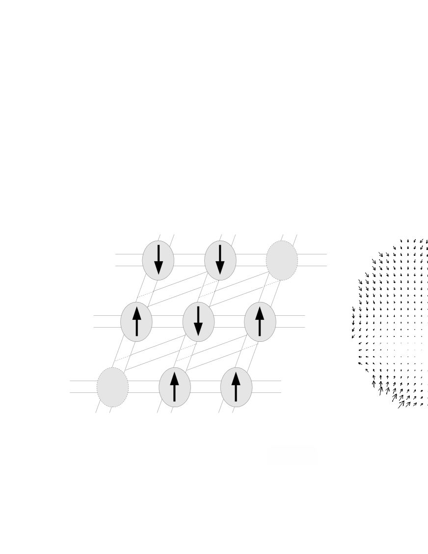
Figure 10: Dipolar configuration. Left: one of the possible magnetic arrangement for the rhomboedric geometry. The dipolar field acting on the central particle is calculated by means of its first and second neighbors. Right: Resulting spatially dependent dipolar field calculated on the central particle.

In general the dipolar field varies in space and is time dependent, which was not considered in Ref [22]. In Fig. 10 we show one possible magnetic configuration for the rhomboedric geometry and the corresponding spatially dependent dipolar field of the central particle. The dipolar field is spatially not uniform, both in strength and direction. The simplest way to study the magneto-dynamics in an array of particles is to consider the spatial average of the dipolar field, without any time dependence. Note that such an approximation is different from the single-spin approximation[22, 23] because the average field is applied to a spatially extended micromagnetic entity. The most complete way to study the magneto-dynamics in an array of particles is to consider the effect of the magnetization rotation of the particle of interest and the movement of the half-selected particles on the dipolar field strength and direction. These motions give rise to the time dependence of the dipolar field.

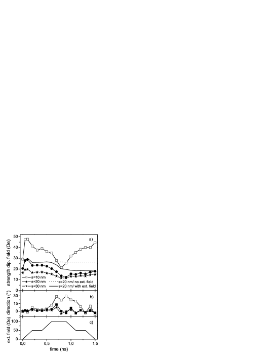
Figure 11: Time-dependent dipolar for various distances between the particles. The field is calculated on the central particle for the configuration of Fig. 10 after application of a pulse with duration $t_{p}$=1.5 ns. a): field strength. b): field direction. c): pulse shape. Legend: Open-square line for s=10 nm. Full-dot line for s=20 nm. Star line for s=30 nm. Dot line (full line): for s=20 nm, dipolar field calculated without (with) application of the external field pulse.

In the following we study the magnetization process of a particle according to the scheme ”g4” and apply the field $H_{sw}=100$ Oe to an elliptical cylinder with $t=1$ nm at zero temperature. The pulse is characterized by (1.5, 0.2, 0.2, 0.8, 0.2). In Fig 11a we plot the time dependence of the dipolar field for the configuration in Fig. 10. The open-square line depicts the time-dependent dipolar field calculated for $s$=10 nm. The value of the dipolar field at $t$=0 corresponds to the one used in the average dipolar field approximation: $\overline{h_{d}}$=29 Oe, where the direction of the sum vector is along the major axis of the ellipse. The increase of the dipolar-field in the first 50 ps is associated to the new minimum reached after relaxation from the starting condition, where the magnetization is imposed to be parallel to the major axis of the ellipse. After that, the magnetization of the fully-selected particle starts to rotate. Such a rotation modifies the orientation of the neighboring particles leading to a decrease of the dipolar field. The minimum is reached after 800 ps. At this moment the average magnetization direction of the fully-selected particle is parallel to the minor axis of the ellipse. Successively, the magnetization turns back into the initial minimum without switching and the dipolar field increases to the value taken before starting the rotation. The full-dot line shows the time dependent dipolar field calculated for $s$=20 nm. The strength of the initial dipolar field is $\overline{h_{d}}$=20.5 Oe, with the direction of the sum vector along the major axis of the ellipse. The behavior of the time-dependent dipolar field is similar to the former case up to 800 ps. However, the fluctuation of the field is smaller than in the other case because the particle separation is larger. For $s$=20 nm the magnetization switches and the dipolar field does not increase to the value taken before starting the rotation. A similar behavior is also found for $s$=30 nm (star line). In that case $\overline{h_{d}}$=16.4 Oe and the fluctuation is again reduced. In Fig 11b we plot the variation of the direction of the dipolar field as a function of time. The direction fluctuations decrease with separation ”s”, like for the strength. In the following we investigate in more details the case with particle separation $s$=20 nm. The dot-line in Fig 11a depicts the relaxation behavior of the central particle magnetization in the presence of the dipolar field without external magnetic field. The dipolar field increases according to the relaxation of the system from the starting state into the energetic minimum. After that, the dipolar field does not change anymore because no external field is applied. In contrast, by applying the switching field the magnetization rotates acting on the neighboring particles and, thus, modifying the time-dependent dipolar field (see full-line). Finally, the contribution of the motion of the half-selected particles is evident by comparing the full-dot line with the full line. In particular, taking this motion into account this leads to a reduction of the strength of the time dependent dipolar field. This reduction has its maximum of 7 Oe at t=800 ps.

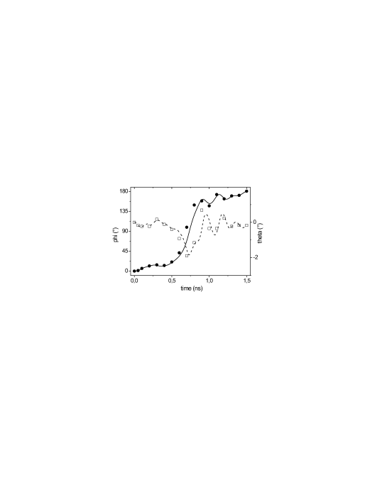
Figure 12: Magnetization trajectory in the presence of the dipolar field. The trajectory refers to the fully-selected particle in Fig. 10 and it is calculated in the presence of either the exact dipolar field (full dot, open square for the components) or the average dipolar field (full and dot line).

In order to simplify the calculation of the switching process and to shorter the simulation time, it is necessary to approximate the spatial and time dependent dipolar field with the averaged dipolar field. Such an approximation drops the simulation time by about a factor of 10. To justify the use of this approximation the difference between the switching processes obtained with the averaged dipolar field and the exact dipolar field has to be small. In Fig. 12 we plot the time-dependence of the components of the average magnetization for the switching process for $s$=20 nm. The trajectory obtained in presence of the exact dipolar field (full-dot line in Fig.  11a) is represented by the full dots and the open squares. In contradistinction, we show with the full and dot lines the components of the average magnetization obtained with the averaged dipolar field. The trajectories behave similarly. The main difference is found during the switching period at t=700 ps signified by a shift of 50 ps between the two trajectories. However, the final states and the majority of points during the switching process coincide. Therefore the use of the averaged dipolar field approximation is justified. Note that for $s$=20 nm the criterion of multi-switching stability is not satisfied because the particle of interest in some of the 32 possible magnetic configurations does not switch. In order to satisfy the criterion the separation has to be larger. To conclude, we have analyzed the difference between the two approaches as a function of the separation and verified that the larger the particle separation the more justified is the use of the averaged dipolar field approximation.

B. Effect of the dipolar interaction on the switching stability

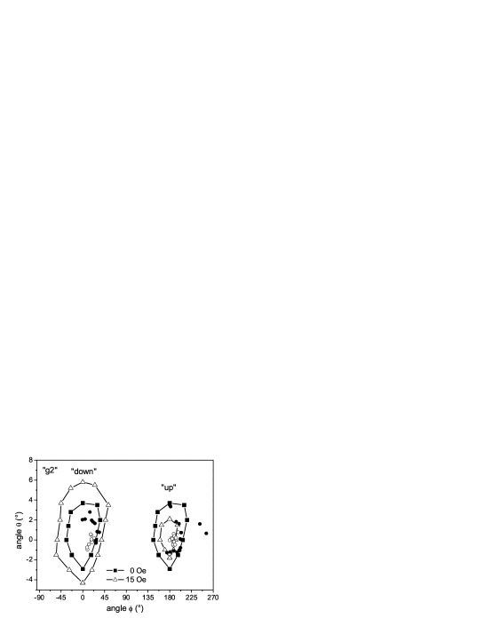
Figure 13: Regions of stability for the addressing scheme ”g2”. Square line: regions calculated in absence of the dipolar interaction. Triangle line: regions calculated in the presence of the averaged dipolar field $\overline{h_{d}}$=15 Oe. Full dots: final states obtained after application of a pulse with duration $t_{p}$=0.7 ns from the ”triangle” points. Open dots: final states obtained after application of a pulse with duration $t_{p}$=1.5 ns from the ”triangle” points.

In the following section we study the effect of the dipolar interaction on the regions of stability and on the magnetization trajectories for particles subjected to the switching schemes ”g2”, ”g3” and ”g4”. According to the results of the previous section we consider particles subjected to an averaged dipolar field calculated by taking into account the first and second neighbors. In order to calculate the averaged dipolar field we assume the particles to be placed on a square grid, which is the usual geometry present in the literature. In absence of the dipolar interaction the particles with thickness $t=2$ nm satisfy the criterion of multi-switching stability both at zero and room temperature (see section III). To study the effect of the dipolar interaction at room temperature we consider the same particle arrangement subjected to magnetic field pulses with strength $H_{sw}=130$ Oe. As mentioned in sec. IIA, the classical switching scheme ”g1” does not guarantee sufficient stability in the presence of the dipolar interaction[5]. According to our procedure, in order to judge the stability for the switching scheme ”g1”, we have to prove the stability of the ”up” and ”down” states under the action of the field h${{}_{\textbf{b}}}$ ($h{{}_{b}}$=122.2 Oe), which is the relevant component of the field h${{}_{\textbf{sw}}}$. In absence of the dipolar interaction we find that an offset $\Delta\theta=0.5^{\circ}$ from the minimum ($\theta=0^{\circ}$,$\phi=180^{\circ}$) is sufficient to cause instability. This value is much smaller than those obtained for the switching schemes ”g2”, ”g3” and ”g4” even in the presence of dipolar interaction, see Figs. 13-14. Furthermore, the magnetization placed in the minimum ($\theta=0^{\circ}$,$\phi=180^{\circ}$) becomes unstable by adding to the field h${{}_{\textbf{b}}}$ a magnetic field $h_{x}$=4 Oe used to simulate the averaged dipolar field. These examples show that the switching scheme ”g1” is inadequate with regard to stability in the presence of the dipolar interaction. We now consider switching scheme ”g2”[7]. In order to find the regions of stability the magnetization is subjected to the field h${{}_{\textbf{a}}}$, see Fig. 1b, which creates a larger torque than the field h${{}_{\textbf{b}}}$ and, thus, is the relevant component of h${{}_{\textbf{sw}}}$ to study the stability. In Fig. 13 we plot the regions of stability calculated for a step function with rise-time $t_{r}$=75 ps and strength $h_{sw}=130$ Oe. Since the magnetic torque $|$M$\times$h${{}_{\textbf{sw}}}$$|$ is invariant for M in the ”up” or in the ”down” state, see sec. II-A, in absence of dipolar interaction the regions of stability are the same. This symmetry is broken in the presence of the dipolar interaction. For the distance $s=130$ nm, the average dipolar field produced on the central particle by the first and second neighbors is $\overline{h_{d}}$=15 Oe, see Fig. 9. Note that this number refers to the ”key”-configuration to study the dipolar coupling, see above in sec. IV-A. Furthermore, for smaller ”s” the averaged dipolar field would inhibit a functioning of the switching scheme ”g2”. Since h${{}_{\textbf{d}}}$ is oriented in the ”down” direction, the stability of the ”down” state increases, while the one of the ”up” state decreases. As a consequence, the area of the stability regions grows or shrinks correspondingly, see Fig. 13. In order to study the switching properties, we compare two different pulses with duration 0.7 ns and 1.5 ns. The pulses are characterized by (0.7, 0.075, 0.1, 0.2, 0.075) and (1.5, 0.075, 0.2, 0.8, 0.075). In absence of the dipolar interaction, for $t_{p}=0.7$ ns some of the trajectories do not terminate inside the stability regions after switching. On the other hand, for $t_{p}=1.5$ ns all the trajectories terminate inside the stability regions and the criterion of multi-switching stability is satisfied. In Fig. 13 we plot the final states obtained after switching in the presence of the dipolar interaction for $\overline{h_{d}}$=15 Oe. In particular, we show with the full dots the states associated to the pulse with duration $t_{p}=0.7$ ns and with the open dots the states associated to the pulse with duration $t_{p}=1.5$ ns. First we consider the switching from the ”up” state into the ”down” state. From Fig. 13 we see that all the trajectories terminate inside the stability region (triangle line). Furthermore, we notice that the dispersion of the final states increases by decreasing the duration of the pulse. By considering the switching from the ”down” into the ”up” state we observe that some of the final states do not end up in the stability region. This happens for both pulse durations. Therefore for the switching scheme ”g2” and for the pulses considered, the criterion of multi-switching stability is not satisfied for $\overline{h_{d}}$=15 Oe.

We now consider switching scheme ”g4” and, according to the procedure presented in section II-B, we calculate the regions of stability for a step function with rise-time $t_{r}$=75 ps and strength $h_{sw}$=130 Oe. In Fig. 14 we plot the resulting regions calculated in absence of the dipolar interaction and in the presence of the averaged dipolar fields $\overline{h_{d}}$=15 Oe and $\overline{h_{d}}$=30 Oe. According to Fig. 9 these fields correspond to arrays of particles with separations $s=130$ nm and $s=82$ nm, respectively. Similar to the result obtained for the switching scheme ”g2”, the effect of the dipolar coupling is to increase the stability of the ”down” state and to decrease the stability of the ”up” state. Since the ”up”-state area is larger than the ”down”-state area, the ”up” state mainly determines the stability of the system. In that sense it is interesting to compare the stability regions of the ”up” state for the switching schemes ”g2” and ”g4”. By comparing Fig. 13 and Fig. 14 we notice that the area of the stability region of the ”up” state obtained with scheme ”g2” for $\overline{h_{d}}$=15 Oe is similar to the one obtained with scheme ”g4” for $\overline{h_{d}}$=30 Oe. Roughly this means that the same results as obtained for the switching scheme ”g2” for an array of particles with separation $s=130$ nm are obtained for the scheme ”g4” for an array of particles with $s=82$ nm. In order to study the switching properties, we compare two pulses with duration 0.7 ns and 1.5 ns. In both cases, in absence of dipolar coupling, all the trajectories terminate inside the stability regions and the criterion of multi-switching stability is satisfied. In the presence of the dipolar interaction all the trajectories from the ”up” state terminate in the ”down” state (see Fig. 14). For $\overline{h_{d}}$=15 Oe with $t_{p}=1.5$ ns all the trajectories from the ”down” state terminate in the ”up” state. Again, the criterion of multi-switching stability is satisfied. On the other hand, for $\overline{h_{d}}$=15 Oe with $t_{p}=0.7$ ns and for $\overline{h_{d}}$=30 Oe with $t_{p}=1.5$ ns, some of the trajectories do not terminate inside the corresponding stability regions. Therefore for the switching scheme ”g4” and for the pulse considered, the criterion of multi-switching stability is not satisfied for $\overline{h_{d}}$=30 Oe.

Finally we consider switching scheme ”g3”. The only difference with scheme ”g1” is the double line ”$b_{1}$” and ”$b_{2}$” used to improve the stability of the half-selected particles. The magnetic field used to calculate the stability regions is $h_{b1}$=$h_{b2}$=61.1 Oe. In Fig. 15 we plot the stability regions obtained in absence of dipolar coupling and in the presence of the averaged dipolar fields $\overline{h_{d}}$=15 Oe and $\overline{h_{d}}$=30 Oe. By comparing Fig. 13 and Fig. 15 we notice that the area of the stability region of the ”up” state obtained for the scheme ”g2” in absence of dipolar coupling is similar to the one obtained for the scheme ”g3” for $\overline{h_{d}}$=30 Oe. Therefore by using the switching scheme ”g3” we expect to have an improvement of stability even higher than with the one obtained by using the switching scheme ”g4”. Such an expectation is confirmed by the study of the switching trajectories. Indeed we find that in the presence of dipolar interaction for $\overline{h_{d}}$=15 Oe with $t_{p}=0.7$ ns and $t_{p}=1.5$ ns and for $\overline{h_{d}}$=30 Oe with $t_{p}=1.5$ ns all the trajectories terminate inside the stability regions, for switchings from the ”up” into the ”down” states and vice-versa. Note also that for all these cases the criterion of multi-switching stability is satisfied.

V. Discussion and conclusion

In this paper we have presented a procedure to study the stability and the switching behavior for an array of magnetic particles. In the literature studies of this type are usually performed with the support of the magnetic astroid. In that case the emphasis is put on the switching aspect of the system. After switching the magnetization is located in the energetic minimum. In the damped regime small misalignments from the minimum do not play an important role for the stability of the system. Therefore in this regime the exact location of the magnetization after switching is not taken into account. Rather, other factors, like the not perfectly equal shape of the particles, the temperature and the dipolar interaction, are decisive to determine the operation margin of the astroid, i. e., the range of stability of the system. On the other hand, in fast dynamics the misalignments dramatically affect the stability of the system (sec. II-B). Therefore it is natural to emphasize the study of the stability of the magnetization, before investigating the switching behavior of the system (II-B). That is what we have done in this paper. First, we have studied the stability of the half-selected particles. Second, we have investigated the switching behavior of the fully-selected particle. This procedure led us to define the criterion of multi-switching stability which has to be satisfied in order to have stable and repeatable switching (II-C). One advantage of this procedure is to give a graphical representation of the intrinsic stability of the system. Since the stability of the system directly depends on the area of the stability regions, to improve the stability one has to enlarge these regions. It is interesting to note that in the literature there are two methods to obtain stable switching in the dynamical regime. One is to prolong the switching time to the time-scale of the damped switching, allowing the magnetization to relax into the energy minimum (magnetization ringing). The other one is to shape the applied magnetic field pulse so that the magnetization reaches directly the minimum without damped relaxation (ballistic precessional switching)[1, 24]. Both methods do not improve the intrinsic stability of the system, i. e., the stability regions do not grow. Comparing now different switching schemes, in this work, in accordance with the literature, we find that the classical addressing scheme ”g1” is not suitable to obtain stable switching. On the other hand, we have shown three alternative schemes, one of which is known from the literature (”g2”), which are suitable to obtain stable switching. The common goal of these schemes is to enlarge the area of the stability regions, either by changing the orientation of the conduction line (”g2”) or by adding a third conduction line (”g3” and ”g4”). Each of these schemes is preferable for some reason. The switching scheme ”g2” works with only two sets of conduction lines. The scheme ”g3” is the most stable in the presence of dipolar interaction. The scheme ”g4” is the only one which uses only unipolar magnetic field pulses. Nevertheless, each of these schemes satisfies the criterion of multi-switching stability at room temperature in the presence of dipolar interaction and for pulses shaped according to CMOS specifications (III, IV-B).

To conclude, we have proved that in an array of magnetic particles it is possible to obtain stable and repeatable switching in the GHz regime. This result has been obtained by improving the stability of the half-selected particles’ magnetization. In accordance with other studies of magneto-dynamics in the fast regime, the magnetization switches by precession. The pulse shaping used in ballistic precessional switching with the aim to exactly ”shoot” the minimum is not required. The magnetization trajectories terminate inside the region of stability, without the necessity to reach a precise point. The switching is precessional, but non-ballistic. We call this non-ballistic precessional switching.

VI. Acknowledgment

The authors thank M. R. Scheinfein for extending his LLG Micromagnetic Simulator[9] to include the position dependent external field tool needed for the present work.

Figure 5: Damped magnetization oscillations vs temperature. The average magnetization relaxes more rapidly at zero temperature than at room temperature. This affects the amplitude of the regions of stability, see Fig.6.

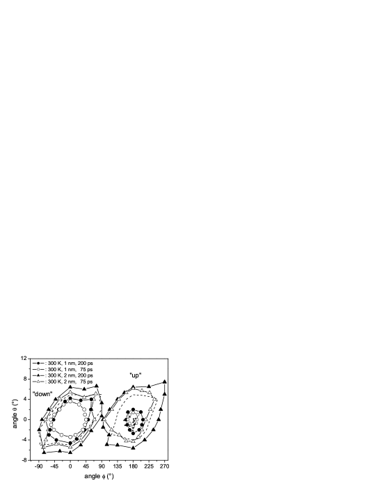
Figure 6: Temperature and rise time dependencies of the stability regions.
Temperature dependence: compare dashed line (zero temperature) with full-dot line (room temperature).
Rise time dependence: compare full-dot/triangle lines ($t_{r}$=200 ps) with open-dot/triangle lines ($t_{r}$=75 ps).
Particle thickness dependence: compare open/close-dot lines (1 nm thickness) with open/close-triangle lines (2 nm thick).
Star-points: final states obtained after switching from the ”down” stability region (open-triangles) for a pulse with duration t=700 ps.

Figure 7: Dispersion index vs. pulse duration. The dispersion of the final states decreases with decreasing the rise time and with increasing pulse duration. See text for details.

Figure 9: Average dipolar field vs. separation of the particles. The value of the field decreases exponentially by increasing the separation. The dipolar coupling is weaker for arrays of cylinder with hight 1 nm (stars) than for arrays of cylinder with hight 2 nm (full dots). The array geometry, either rhomboedric or squared, influence the strength of the dipolar coupling only for small separation of the cylinders (compare full dots with open square).

Figure 14: Regions of stability for the addressing scheme ”g4”. Square line: regions calculated in absence of the dipolar interaction. Triangle line: regions calculated in the presence of the averaged dipolar field $\overline{h_{d}}$=15 Oe. Full-dot line: regions calculated in the presence of the average dipolar field $\overline{h_{d}}$=30 Oe. Full dots: final states obtained after application of a pulse with duration $t_{p}$=0.7 ns from the ”triangle” points. Open dots: final states obtained after application of a pulse with duration $t_{p}$=1.5 ns from the ”triangle” points. Open squares: final states obtained after application of a pulse with duration $t_{p}$=1.5 ns from the ”dot” points.

Figure 15: Regions of stability for the addressing scheme ”g3”. Square line: regions calculated in absence of the dipolar interaction. Triangle line: regions calculated in the presence of the average dipolar field $\overline{h_{d}}$=15 Oe. Full-dot line: regions calculated in the presence of the average dipolar field $\overline{h_{d}}$=30 Oe. Full dots: final states obtained after application of a pulse with duration $t_{p}$=0.7 ns from the ”triangle” points. Open dots: final states obtained after application of a pulse with duration $t_{p}$=1.5 ns from the ”triangle” points. Open squares: final states obtained after application of a pulse with duration $t_{p}$=1.5 ns from the ”dot” points.

References

- [1] J. Miltat, G. Albuquerque, and A. Thiaville, Top. Appl. Phys. 83, 1 (2002).
- [2] G. Bertotti, I. Mayergoyz, C. Serpico, and M. Dimian, J. Appl. Phys. 93, 6811 (2003).
- [3] M. Bauer, J. Fassbender, and. B. Hillebrands, Phys. Rev. B 61, 3410 (2000).
- [4] M. Bauer, R. Lopusnik, J. Fassbender, and B. Hillebrands, Appl. Phys. Lett. 76, 2758 (2000); S. Kaka and S. E. Russek, Appl. Phys. Lett. 80, 2958 (2002).
- [5] T. M. Maffitt, J. K. DeBrosse, J. A. Gabric, E. T. Gow, M. C. Lamorey, J. S. Parenteau, D. R. Willmott, M. A. Wood and W. J. Gallagher, IBM J. Res. Dev. 50, 25 (2006).
- [6] B.N Engel, J. Akerman, B. Butcher, R. W. Dave, M. DeHerrera, M. Durlam, G. Grynkewich, J. Janesky, S. V. Pietambaram, N. D. Rizzo, J. M. Slaughter, K. Smith, J. J. Sun and S. Tehrani, IEEE Trans. Magn. 41, 132 (2005).
- [7] Patent No.: US 6,674,662 B1; M. Bauer, J. Fassbender, B. Hillebrands and R. L. Stamps, Phys. Rev. B 61, 3410 (2000).
- [8] M. Brockmann, S. Miethaner, R. Onderka, M. Köhler, F. Himmelhuber, H. Regensburger, F. Bensch, T. Schweinböck, and G. Bayreuther, J. Appl. Phys. 81, 5047 (1997).
- [9] See http://llgmicro.home.mindspring.com
- [10] A. Thiaville, Phys. Rev. B 61, 12221 (2000).
- [11] C. Maunoury, T. Devolder, C. K. Lim, P. Crozat, and C. Chappert, J. Appl. Phys. 97, 074503 (2005).
- [12] H. W. Schumacher, Appl. Phys. Lett. 87, 042504 (2005).
- [13] J. L. Garcia-Palacios and F. J. Lazaro, Phys. Rev. B 22, 14937 (1998).
- [14] J. G. Deak, J. Appl. Phys. 93, 6814 (2003).
- [15] R. P. Cowburn, J. Phys D 33, R1 (2000).
- [16] T. J. Bromwich, A. Kohn, A. K. Petford-Long, T. Kasama, R. E. Dunin-Borkowski, S. B. Newcomb and C. A. Ross, J. Appl. Phys. 98, 053909 (2005).
- [17] F. Porrati and M. Huth, J. Magn. Magn. Mater. 290, 145 (2005).
- [18] K. Yu Guslienko, Appl. Phys. Lett. 76, 3609 (2000).
- [19] F. Porrati and M. Huth, Appl. Phys. Lett. 85, 3157 (2004).
- [20] R. E. Dunin-Borkowski, M. R. McCartney, B. Kardynal, D. J. Smith, M. R. Scheinfein, Appl. Phys. Lett. 75, 2641 (1999).
- [21] M. C. Abraham, H. Schmidt, T. A. Savas, H. I. Smith, C. A. Ross, R. J. Ram, J. Appl. Phys. 89, 5667 (2001).
- [22] T. Devolder and C. Chappert, J. Appl. Phys. 95, 1933 (2004).
- [23] H. N. Pham, I. Dumitru, A. Stancu and L. Spinu, J. Appl. Phys. 97, 10P106 (2005).
- [24] T. Gerrits, H. A. M. van den Berg, J. Hohlfeld, L. Bär, and T. Rasing, Nature 418, 509 (2002); H. W. Schumacher, C. Chappert, P. Crozat, R. C. Sousa, P. P. Freitas, and M. Bauer, Appl. Phys. Lett. 80, 3781 (2002); H. W. Schumacher, C. Chappert, R. C. Sousa, P. P. Freitas, and J. Miltat, Phys. Rev. Lett. 90, 017204 (2003)