Structure Learning in Nested Effects Models

Abstract

Nested Effects Models (NEMs) are a class of graphical models introduced to analyze the results of gene perturbation screens. NEMs explore noisy subset relations between the high-dimensional outputs of phenotyping studies, e.g. the effects showing in gene expression profiles or as morphological features of the perturbed cell.

In this paper we expand the statistical basis of NEMs in four directions: First, we derive a new formula for the likelihood function of a NEM, which generalizes previous results for binary data. Second, we prove model identifiability under mild assumptions. Third, we show that the new formulation of the likelihood allows to efficiently traverse model space. Fourth, we incorporate prior knowledge and an automated variable selection criterion to decrease the influence of noise in the data.

This manuscript will appear in Statistical Applications in Genetics and Molecular Biology at http://www.bepress.com/sagmb/

1 Introduction

Functional genomics has a long tradition of inferring the inner working of a cell through analysis of its response to various perturbations. There are several perturbation techniques suitable for large-scale analysis in different organisms. Experiments with gene knock-outs have been very successful in uncovering gene function (Hughes et al.,, 2000), and gene silencing by RNA interference (Fire et al.,, 1998) allows perturbation screens on a genome-wide scale.

The changes observed in the cell are called the phenotype of the perturbation. In most biological studies, perturbation effects are measured by single reporters like cell death or growth. Analysis of these phenotypes can reveal which genes are essential for an organism (Boutros et al.,, 2004) or for a particular pathway (Gesellchen et al.,, 2005). However, these screens do not reveal how the genes contribute to regulatory networks or signalling pathways.

More details about gene function and interactions are contained in high-dimensional phenotypes that give a global view of changes in the cell. High-dimensional phenotypes include gene expression profiles (Hughes et al.,, 2000; Boutros et al.,, 2002; Driessche et al.,, 2005), metabolite concentrations (Raamsdonk et al.,, 2001), sensitivity to cytotoxic or cytostatic agents (Brown et al.,, 2006), or morphological features of the cell (Ohya et al.,, 2005). While high-dimensional phenotypic profiles promise a comprehensive view of the function of genes in a cell, only limited work has been done so far to adapt statistical and computational methodologies to the specific needs of large-scale and high-dimensional phenotyping screens.

Phenotypic profiles offer only indirect information

A key obstacle to inferring genetic networks from high-dimensional perturbation screens is that phenotypic profiles generally offer only indirect information on how genes interact. Cell morphology or sensitivity to stresses are global features of the cell, which are hard to relate directly to the genes contributing to them. Gene expression phenotypes also offer an indirect view of pathway structure due to the high number of post-transcriptional regulatory events like protein modifications. For example, when silencing a kinase we might not be able to observe changes in the activation states of other proteins involved in the pathway. The only information we may get is that genes downstream of the pathway show expression changes. Thus, phenotypic profiles may provide only an indirect view of information flow and pathway structure in the cell.

Statistical analysis of phenotyping screens

Previous work focused on clustering phenotypic profiles to find groups of genes that show similar effects when perturbed. The rationale is that genes with similar perturbation effects are expected to be functionally related. The most prominent method used is average linkage hierarchical clustering (Piano et al.,, 2002; Ohya et al.,, 2005). A complementary approach is ranking genes according to similarity with a query gene (Gunsalus et al.,, 2004). In a supervised setting, first steps have been taken to classify genes into functional groups based on phenotypic profiles (Ohya et al.,, 2005). A comprehensive overview of computational models for the reconstruction of genetic networks can be found in (Markowetz and Spang,, 2007).

A recent approach especially designed to learning from indirect information and high-dimensional phenotypes are Nested Effects Models (Markowetz et al.,, 2005, 2007) that reconstruct features of the internal organization of the cell from the nested structure of observed perturbation effects. Perturbing some genes may have an influence on a global process, while perturbing others affects sub-processes of it. Imagine, for example, a signaling pathway activating several transcription factors. Blocking the entire pathway will affect all targets of the transcription factors, while perturbing a single downstream transcription factor will only affect its direct targets, which are a subset of the phenotype obtained by blocking the complete pathway. NEMs can be seen as a generalization of similarity-based clustering, which orders (clusters of) genes according to subset relationships between the sets of phenotypes. So far, a likelihood function has been derived for NEMs in the case of discretized or binary data (Markowetz et al.,, 2005) and $p$-values of differential expression (Fröhlich et al., 2007a, ). For model inference, divide-and-conquer strategies have been applied to scale up model search (Markowetz et al.,, 2007; Fröhlich et al., 2007b, ).

Overview of this paper

After introducing a generalized version of NEMs in Section 2 we expand their statistical basis in four directions: First, we derive a new formula for the likelihood function of a NEM that generalizes previous results (Section 3). Second, we prove model identifiability under mild assumptions (Section 4). Third, we develop efficient methods of traversing model space (Section 5). And finally, we incorporate prior knowledge and a variable selection step into model search to decrease the influence of noise in the data (Section 6). We show the applicability of the proposed method in the controlled setting of a simulation scenario (Section 7) and in an application to an example in Drosophila immune response (Section 8).

2 Definition of nested effects models

The system of components we consider consists of a set $\mathcal{O}$ of $n_{\mathcal{O}}$ observable entities (e.g. mRNA concentrations), and a set $\mathcal{A}$ of $n_{\mathcal{A}}$ actions (i.e. gene perturbations) applied to the system which are expected to alter the state of some observable entities. Both $\mathcal{O}$ and $\mathcal{A}$ consist of binary variables. An altered state of an observable $s\in\mathcal{O}$ is denoted by $s=1$, the basic state is $s=0$. A value of $a=1$, resp. $a=0$, means that action $a\in\mathcal{A}$ was performed, resp. not performed. Let $D_{as}$, $(a,s)\in\mathcal{M}\subseteq\mathcal{A}\times\mathcal{O}$ be a set of measurements for observation $s$ after performing action $a$. The set of all measurements $D=\{D_{as}\,|\,(a,s)\in\mathcal{M}\}$ constitutes the data. Note that our definition of $\mathcal{M}$ does not require that all $s\in\mathcal{O}$ are observed for all actions $a\in\mathcal{A}$. Thus, missing data and the exclusion of failed experiments can directly be incorporated into all the results that we develop in the following.

Definition 1.

A (general) effects model is a binary $n_{\mathcal{A}}\times n_{\mathcal{O}}$ matrix $F$ that determines the state of the observable $s$ when action $a$ is performed, an entry $0$ indicating no change, $1$ indicating a change.

Nested effects models are effects models that can be defined in terms of two graphs or adjacency matrices. The first graph, $\Gamma$, describes how actions imply each other and the second graph, $\Theta$, how observables are linked to actions. Let the actions graph $\Gamma=(\Gamma_{aa^{\prime}})$ be a graph on the vertices $\mathcal{A}$ , encoded as an $n_{\mathcal{A}}\times n_{\mathcal{A}}$ adjacency matrix with the convention $\Gamma_{aa}=1$, $a\in\mathcal{A}$. We say that the edge $a\to a^{\prime}$ is in $\Gamma$, or for short $a\stackrel{{\scriptstyle\Gamma}}{{\to}}a^{\prime}$, if $\Gamma_{aa^{\prime}}=1$.

Secondly, we assume that each observation is directly linked to exactly one action as defined by a function $\theta:\mathcal{O}\to\mathcal{A}$. This can synonymously be encoded as an $n_{\mathcal{A}}\times n_{\mathcal{O}}$ adjacency matrix $\Theta=(\Theta_{as})$, with $\Theta_{as}=\delta_{a=\theta(s)}$ for $a\in\mathcal{A}$, $s\in\mathcal{O}$ (where $\delta_{\cdot}$ is the delta function). Write $a\stackrel{{\scriptstyle\Theta}}{{\to}}s$ if $\Theta_{as}=1$. By this definition, $\Theta$ contains only zeros except for a single $1$ in each column. When describing how observables are linked to actions, we tacitly switch between the adjacency matrix $\Theta$ and the function $\theta$ for the sake of notational convenience.

We postulate an effect of an action $a\in\mathcal{A}$ on $s\in\mathcal{O}$ if and only if there exists an action $a^{\prime}\in\mathcal{A}$ such that the edge from $a$ to $a^{\prime}$ is in $\Gamma$, and $s$ is directly linked to $a^{\prime}$ (the edge from $a^{\prime}$ to $s$ is in $\Theta$). Since each observable is linked to exactly one action, action $a$ has an effect on $s$ if and only if $(\Gamma\Theta)_{as}=1$. This prompts the following definition:

Definition 2.

A nested effects model (NEM) $F$ is an effects model which can be represented as a product of $\Gamma$ and $\Theta$ as defined above:

$$F\ =\ \Gamma\,\Theta.$$ (2.1)

The parameters $\Gamma$ and $\Theta$ uniquely determine the model. We therefore use $P(D\,|\,\Gamma,\Theta)$ interchangeably with $P(D\,|\,F)$. Examples of nested effects models are given in Fig. 1, showing the graphs $\Gamma$ and $\Theta$ as well as the resulting effects model $F$.

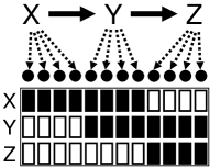
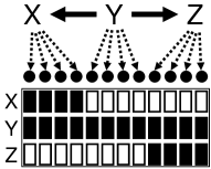
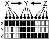
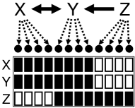
Figure 1: NEM examples. Each plot shows a NEM on $\mathcal{A}=\{X,Y,Z\}$ and twelve observables $\mathcal{O}$ depicted as dots. The solid arrows define the adjacency matrix $\Gamma$. Note that cyclic graphs are allowed, like the right-most example which contains a bi-directional edge. Each action in $\mathcal{A}$ is connected to observables $s\in\mathcal{O}$ by dashed arrows encoding $\Theta$ (which is assumed fixed in all three plots). The lower parts of the plots show the model matrix $F$ in each of these three cases. Each cell in the matrix corresponds to the state of one observable $s\in\mathcal{O}$ after performing an action $a\in\mathcal{A}$. Cells containing observed effects are colored black, those containing non-effects are white. The objective of structure learning in NEMs is to recover $\Gamma$ and $\Theta$ from noisy observations of effect patterns.

Transitivity requirement

Previous definitions of NEMs required the actions graph to be transitively closed (Markowetz et al.,, 2005, 2007), restricting model space from the space of all graphs to the space of transitively closed graphs. This is sensible if paths in the actions graph are interpreted as causal chains. For transitively closed graphs, our model has a property that motivated the name “nested effects model”: The existence of an edge $a\rightarrow a^{\prime}$ in a transitively closed graph implies that the effects observed for action $a^{\prime}$ (i.e. all effects $s$ with $\theta(s)=a^{\prime}$) are “nested” in the observed effects of $a$:

$$a\stackrel{{\scriptstyle\Gamma}}{{\to}}a^{\prime}\quad\Leftrightarrow\quad\{s\in\mathcal{O}\,|\,F_{a^{\prime}s}=1\}\subseteq\{s\in\mathcal{O}\,|\,F_{as}=1\}.$$ (2.2)

This correspondence induces an order homomorphism from $\Gamma$ to the subset lattice of the set observations, which is satisfactory from a mathematical point of view.

However, admitting only transitively closed graphs as valid models is a constraint which makes structure learning computationally hard (Markowetz et al.,, 2007). Even a small change in the model—like removing or adding an edge—can make many more changes necessary to preserve transitivity. The likelihood function will be quite volatile and the likelihood landscape will not be smooth.

Our calculations here do not rely on the transitivity of the actions graph. Our definition of NEMs thus extends the one used in previous studies (Markowetz et al.,, 2005, 2007; Fröhlich et al., 2007a, ; Fröhlich et al., 2007b, ).

3 Inference of the actions graph

Likelihood

Assuming data independence, the likelihood of the model $F$ (with data $D$ fixed) factors into

$$P(D|F)\ = \prod_{(a,s)\in\mathcal{M}}\!\!P(D_{as}\,|\,s=F_{as})$$ (3.1)

$$\propto \prod_{(a,s)\in\,\mathcal{O}\times\mathcal{A}}\!\!\!\!P(D_{as}\,|\,s=F_{as})$$ (3.2)

$$\text{or\ \ \ \ \ }\log P(D|F)\ = \sum_{(a,s)\in\,\mathcal{A}\times\mathcal{O}}\!\!\!\!\log\,P(D_{as}\,|\,s=F_{as})\ \ +\ const,$$ (3.3)

if we define $P(s=x|a)=0.5$ for $x\in\{0,1\}$ and $(a,s)\in(\mathcal{A}\times\mathcal{O})\setminus\mathcal{M}$. The quantity $\log P(D|F)$ can be expressed in a convenient form: For an observable $s\in\mathcal{O}$ and a perturbation $a\in\mathcal{A}$, let the log likelihood ratio $R_{sa}=\log\frac{P(D_{as}\,|\,s=1)}{P(D_{as}\,|\,s=0)}$ be known, and $R=(R_{sa})$ be the $\mathcal{O}\times\mathcal{A}$ matrix of ratios. If we let $N$ be the null matrix, i.e. the model predicting no effects at all, then

$$\log P(D|F)-\log P(D|N) \underset{(\ref{loglikelihood})}{=} \sum_{(a,s)\in\,\mathcal{A}\times\mathcal{O}}log\,\frac{P(D_{as}\,|\,s=F_{as})}{P(D_{as}\,|\,s=0)}$$

$$= \sum_{(a,s)\in\,\mathcal{A}\times\mathcal{O}}\left\{\!\begin{tabular}[]{cl}$R_{sa}$\!\!&if $F_{as}=1$\\ $0$&if $F_{as}=0$\end{tabular}\right.$$

$$= \sum_{a\in\mathcal{A}}\sum_{s\in\,\mathcal{O}}F_{as}R_{sa}$$

$$= \sum_{a\in\mathcal{A}}(FR)_{aa}\ =\ tr\,(FR)\ \ ,$$ (3.7)

with “$tr$” denoting the trace function of a quadratic matrix. This derivation of the likelihood applies to both general effects models and nested effects models. In particular, in nested effects models Eq. (2.1) allows to represent the likelihood as

$$\log P(D|\Gamma,\theta)\ =\ tr(\Gamma\Theta R)\ +\ const\ .$$ (3.8)

The likelihood function depends on the data only via the likelihood ratios in $R$. This makes our approach very flexible: our method can handle as input data binary values, $p$-values, or any other arbitrary statistic as long as it can be converted to a likelihood ratio. Section 8 contains an outline of how this quantity can be estimated in a practical application to gene expression microarray data.

Posterior

We aim at maximizing the posterior of $\Gamma$ and $\Theta$,

$$P(\Gamma,\Theta\,|\,D) = \frac{P(D\,|\,\Gamma,\Theta)\cdot P(\Gamma,\Theta)}{P(D)}$$ (3.9)

$$\propto P(D\,|\,\Gamma,\Theta)\cdot P(\Gamma)\cdot P(\Theta),$$

where we assume that the parameters $\Gamma$ and $\Theta$ are independent and follow prior distributions $P(\Gamma)$ amd $P(\Theta)$, which are not necessarily uniform.

Let $Q=(Q_{sa})$ be an $n_{\mathcal{O}}\times n_{\mathcal{A}}$ matrix with entries $Q_{sa}=P(\theta(s)=a)$. We assume that the prior links each observation independently to an action, i.e.

$$P(\Theta)=\prod_{s\in\mathcal{O}}P(\theta(s)=a_{s})\ \ \ \text{or}\ \ \ \log P(\theta)=\sum_{s\in\mathcal{O}}Q_{sa_{s}}$$ (3.10)

where $a_{s}$ is the particular value of $\theta(s)$ in $\Theta$. Consider the data $D$ fixed and write $L(\Gamma,\theta)=\log P(D\,|\,\Gamma,\theta)$ for the log-likelihood of the data, given the model. Then the posterior of the model $(\Gamma,\theta)$ becomes

$$\log P(\Gamma,\theta\,|\,D) \underset{(\ref{posterior})}{=} L(\Gamma,\theta)\ +\ \log P(\Gamma)\ +\ \log P(\theta)\ +\ const$$ (3.11)

The task is to find the MAP estimate for $P(\Gamma,\Theta\,|\,D)$,

$$(\hat{\Gamma},\hat{\theta}) = \underset{\Gamma,\theta}{\operatorname*{argmax}}\big{(}\,L(\Gamma,\theta)+\log P(\Gamma)+\log P(\theta)\,\big{)}$$ (3.12)

We are particularly interested in finding the optimal actions graph $\hat{\Gamma}$. Writing

$$\theta_{\Gamma} = \underset{\theta}{\operatorname*{argmax}}\,\big{(}L(\Gamma,\theta)+\log P(\theta)\big{)}\ \text{,}$$ (3.13)

$$L(\Gamma) = L(\Gamma,\theta_{\Gamma})=\underset{\theta}{\text{max}}\,L(\Gamma,\theta)\ ,$$ (3.14)

this corresponds to finding

$$\hat{\Gamma} = \underset{\Gamma}{\operatorname*{argmax}}\big{(}\,\underset{\theta}{\text{max}}\big{(}L(\Gamma,\theta)+\log P(\theta)\big{)}+\log P(\Gamma)\,\big{)}$$ (3.15)

$$= \underset{\Gamma}{\operatorname*{argmax}}\big{(}\,L(\Gamma)+\log P(\Gamma)\,\big{)}$$

4 Model identifiability

We present theorems showing that the maximum likelihood estimator recovers the true structure of the actions graph for sufficiently “good” data. All proofs are given in the appendix.

Definition 3.

Let some data be observed from the underlying true effects model $F$. Let $R$ be the ratio matrix which has been derived from the data. We say that the data is consistent with $F$ if the ratio matrix $R$ has a positive entry $R_{sa}$ (= favors an effect) whenever $F$ has a positive entry $F_{as}$ (= predicts an effect) at the corresponding position.

Theorem 1.

If the data is consistent with the effects model $F$, then the maximum likelihood estimate of (3) equals $F$,

$$F=\ \underset{G}{\operatorname*{argmax}}\ P(D|G)\ \underset{(\ref{trace1})}{=}\ \underset{G}{\operatorname*{argmax}}\ tr(GR)\ .$$ (4.1)

$\Box$

In the light of this theorem it is interesting to find out to what extent the actions graph $\Gamma$ and the assignment $\Theta$ are controlled by the nested effects model $F=\Gamma\Theta$. The complete answer is given in Theorem 3. We precede it by a definition and a lemma.

Definition 4.

Let $F$ be a nested effects model parametrized by $(\Gamma,\Theta)$. Let $a_{1}\to a_{2}\to...\to a_{n}\to a_{1}$ be a cycle in $\Gamma$, let $\pi$ be the circular permutation $\pi=(a_{1}\,a_{2}...a_{n})$. Let $e_{b}$ denote the $b$-th unit column vector of length $n_{\mathcal{O}}$, and let $S=\sum_{b\in\mathcal{A}}e_{b}e^{T}_{\pi(b)}$ be the permutation matrix corresponding to $\pi$. We say that $(\Gamma^{\prime},\Theta^{\prime})=(\Gamma S^{-1},S\Theta)$ is a reversal of $(\Gamma,\Theta)$ induced by $\pi$ (see Fig. 2 for an example). Two reversals are called disjoint if they are induced by disjoint cyclic permutations (i.e. each action is fixed by at least one of the permutations).

Lemma 2.

Let $(\Gamma^{\prime},\Theta^{\prime})$ be a reversal of $(\Gamma,\Theta)$ induced by the permutation $\pi=(a_{1},a_{2},...,a_{n})$. Then $(\Gamma^{\prime},\Theta^{\prime})$ is a valid parametrization of $F=\Gamma\Theta$.

Lemma 2 states that the two parametrizations $(\Gamma,\Theta)$ and $(\Gamma^{\prime},\Theta^{\prime})$ define the same nested effects model, thus we call them observationally equivalent.

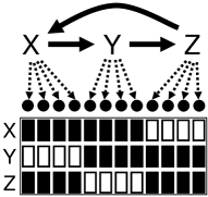
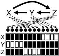
Figure 2: A basic example of a reversal. Both plots show a NEM on $\mathcal{A}=\{X,Y,Z\}$ and twelve observables $\mathcal{O}$ depicted as dots. The actions graphs $\Gamma$ and ${\Gamma}^{\prime}$ are both cyclic, but the two models differ in the direction of the cycle (clock-wise on the right, against the clock on the left). However, the two model matrices $F$ and $F^{\prime}$ are identical, since the change from $\Gamma$ to ${\Gamma}^{\prime}$ can be compensated by simultaneously changing the assignment between actions and observables (indicated by the dashed arrows).

For an action $a\in\mathcal{A}$, the parents of $a$ are the actions $b\in\mathcal{A}$ such that $b\stackrel{{\scriptstyle\Gamma}}{{\to}}a$. If two distinct actions $a,b\in\mathcal{A}$ have the same parents, then they are clearly indistinguishable by any kind of interventional measurement. This is a general limitation, not only a limitation of our model. We propose collapsing these two actions in such a case (Markowetz et al.,, 2007). We exclude indistinguishable actions from our considerations and state:

Theorem 3.

Let $(\Gamma,\Theta)$ and $(\Gamma^{\prime},\Theta^{\prime})$ be the parameters of two nested effects models. Assume that no two distinct actions $a,b\in\mathcal{A}$ have the same parents in $\Gamma$ or in $\Gamma^{\prime}$. Then $(\Gamma,\Theta)$ and $(\Gamma^{\prime},\Theta^{\prime})$ are observationally equivalent if and only if the tuples can be converted one into another by a sequence of disjoint reversals. $\Box$

Taken together, Theorems 1 and 3 state that under mild conditions, not only the true nested effects model $F$ is identifiable for ”sufficiently good” data (which in practical cases means for a sufficiently high number of replicate measurements), but also the underlying actions graph $\Gamma$ and the assignment $\theta$ are unique up to reversals.

5 Actions graph search

The space $\mathfrak{G}$ of actions graphs is huge, it contains $2^{n_{\mathcal{A}}(n_{\mathcal{A}}-1)}$ elements (recall that the diagonal entries of the adjacency matrix equal $1$ ). In order to search $\mathfrak{G}$ efficiently, we need a fast method for the evaluation of (3.9). The key observation is that small changes in $\Gamma$ require only small changes in the optimal assignment $\theta$, and these can be calculated very fast.

Elementary moves

Let $\Gamma$ and $\Gamma^{\prime}$ be neighbours in $\mathfrak{G}$ , i.e. $\Gamma$ and $\Gamma^{\prime}$ differ exactly in one edge, from action $j$ to action $k$ say. An elementary move is defined as the insertion or the removal of one edge in an actions graph (note that if we chose the search space $\mathfrak{G}$ to be the transitively closed graphs or the acyclic graphs, these moves would not be well defined). Let $e_{j}$ denote the $j$-th unit column vector of length $n_{\mathcal{O}}$, and let $g_{k}$ be the $k$-th unit column vector of length $n_{\mathcal{A}}$. By $x^{T}$ denote the transpose of a vector or a matrix $x$. Define $E_{jk}=e_{j}e_{k}^{T}$ as the matrix containing only zero entries except a $1$ in row $j$, column $k$. Then

$$\Gamma^{\prime}=\Gamma+\epsilon_{jk}E_{jk}\ ,\ \ \text{where}\ \ \ \epsilon_{jk}=1-2\Gamma\!\!_{jk}.$$ (5.1)

Optimization of the effects graph

Let $G_{js}=e_{j}g_{s}^{T}$, $j\in\mathcal{A}$, $s\in\mathcal{O}$. Then

$$L(\Gamma,\theta)-L(f_{0}) \underset{(\ref{trace2})}{=} tr(\Gamma\Theta R)$$ (5.2)

$$= tr(\Gamma(\sum_{s\in\mathcal{O}}G_{\theta(s),s})R)=\sum_{s\in\mathcal{O}}tr(\Gamma G_{\theta(s),s}R)$$

$$= \sum_{s\in\mathcal{O}}tr(\Gamma e_{\theta(s)}\cdot g_{s}^{T}R)=\sum_{s\in\mathcal{O}}tr(\Gamma_{\cdot\theta(s)}R_{s\cdot})=\sum_{s\in\mathcal{O}}tr(R_{s\cdot}\Gamma_{\cdot\theta(s)})$$

$$= \sum_{s\in\mathcal{O}}R_{s\cdot}\Gamma_{\cdot\theta(s)}=\sum_{s\in\mathcal{O}}(R\Gamma)_{s\theta(s)}$$

It follows from the equations (3.10),(3.13) and (5.2) that maximizing $\theta$ with respect to $L(\Gamma,\theta)$ can be done pointwise, i.e.

$$\theta_{\Gamma}(s)=\underset{a\in\mathcal{A}}{\operatorname*{argmax}}\big{(}(R\Gamma)_{sa}+Q_{sa}\big{)}\ ,\ \ s\in\mathcal{O}.$$ (5.3)

For each $s\in\mathcal{O}$, step (5.3) takes $\text{\bf O}(n_{\mathcal{O}})$ time, provided that the matrix $R\Gamma$ is given. It is therefore necessary to keep track of this matrix whenever $\Gamma$ is changed into a $\Gamma^{\prime}$. But $R\Gamma^{\prime}=R\Gamma+\epsilon_{jk}RE_{jk}$ is obtained from $R\Gamma$ simply by adding $\epsilon_{jk}R.j$ to the $k$-th column of $R\Gamma$, so this process takes only $\text{\bf O}(n_{\mathcal{A}})$ time. The complete evaluation of $\theta$ according to (5.3) takes $\text{\bf O}(n_{\mathcal{A}}n_{\mathcal{O}})$ time. However we can exploit the fact that (in expectation) hardly any of the observable effects has to be reassigned. For the moment, fix $s\in\mathcal{O}$ and consider the vector $v=(R\Gamma)_{s\cdot}+Q_{s\cdot}$ and let

$$w = (R\Gamma^{\prime})_{s\cdot}+Q_{s\cdot}=\left(R(\Gamma+\epsilon_{jk}E_{jk})\right)_{s\cdot}+Q_{s\cdot}$$ (5.4)

$$= \left((R\Gamma)_{s\cdot}+\epsilon_{jk}(Re_{j}e_{k}^{T}\right)_{s\cdot})+Q_{s\cdot}$$

$$= v+\epsilon_{jk}(e_{s}^{T}Re_{j})e_{k}^{T}=v+\epsilon_{jk}R_{sj}e_{k}^{T}\ .$$

By (5.3), $t=\theta_{\Gamma}(s)=\operatorname*{argmax}_{a\in\mathcal{A}}v_{a}$ and $\theta_{\Gamma^{\prime}}(s)=\operatorname*{argmax}_{a\in\mathcal{A}}w_{a}$. The vector $v$ differs from $w$ at most in its $k$-th entry. The following cases can occur:

$$\theta_{\Gamma^{\prime}}(s) = \left\{\begin{tabular}[]{cl}$t$&\text{if $t\neq k$ , $w_{k}\leq v_{t}$}\\ $k$&\text{if $t\neq k$ , $w_{k}>v_{t}$}\\ $k$&\text{if $t=k$ , $w_{k}\geq v_{k}$}\\ $\underset{a\in\mathcal{A}}{\operatorname*{argmax}}\,w_{a}$&\text{if $t=k$ , $w_{k}<v_{k}$}\end{tabular}\right.$$ (5.9)

$$= \!\left\{\begin{tabular}[]{cl}$t$&\text{if $t\neq k$ , $v_{k}+\epsilon_{jk}R_{sj}\leq v_{t}$}\\ $k$&\text{if $t\neq k$ , $v_{k}+\epsilon_{jk}R_{sj}>v_{t}$}\\ $k$&\text{if $t=k$ , $\epsilon_{jk}R_{sj}\geq 0$}\\ $\underset{a\in\mathcal{A}}{\operatorname*{argmax}}\,w_{a}$&\text{if $t=k$ , $\epsilon_{jk}R_{sj}<0$}\end{tabular}\right.$$ (5.14)

Given the matrix $R\Gamma$, the first three cases in (5.9) can be calculated in constant time. The fourth case requires $\text{\bf O}(n_{\mathcal{A}})$ time. The elementary moves choose every edge $j\to k$ with the same frequency, so the expected relative frequency for which the case $t=k$ occurs is $\frac{1}{n_{\mathcal{A}}}$. Therefore, the expected running time for (5.9) is at most $\text{\bf O}(\frac{n_{\mathcal{A}}-1}{n_{\mathcal{A}}}\cdot 1+\frac{1}{n_{\mathcal{A}}}\cdot n_{\mathcal{A}})=\text{\bf O}(1)$. We have to do this step for all $s\in\mathcal{O}$, so the calculation of the function $\theta$ can be done in expected $\text{\bf O}(n_{\mathcal{O}})$ time. What remains to do is to update the matrix $R\Gamma$ to

$$R\Gamma^{\prime}=R\Gamma+\epsilon{jk}RE_{jk}=R\Gamma+\epsilon_{jk}R_{\cdot j}e_{k}^{T}\ .$$

This only affects the $k$-th column of $R\Gamma$, to which we add the vector $\epsilon_{jk}R_{\cdot j}$. The time consumption of this step is $\text{\bf O}(n_{\mathcal{O}})$.

Gray code enumeration of actions graphs

Actions graphs are treated as binary vectors of length $n_{\mathcal{A}}^{2}-n_{\mathcal{A}}$ (the diagonal is fixed), and they are enumerated without redundances using a gray code (Knuth,, 2005). Each enumeration step alters exactly one edge of the predecessor graph, so we can take advantage of our fast update algorithm. It allows the exhaustive search of the actions graph space $\mathfrak{G}$ for $n\leq 5$ (computation time on a 1GHz computer: a few seconds for $n=4$ actions, approx. 10mins for $n=5$ actions).

6 Extensions

In this section, we adapt the raw nested effects model to make it more applicable to real-life data sets. We discuss methods to incorporate prior knowledge on parts of an action graph and to decrease measurement noise by feature selection and regularization.

6.1 Rigid actions graph prior

In many practical applications, parts of the true actions graph structure is already known, and only a fraction of edges has to be estimated from the data. Taking advantage of this, we introduce a rigid prior on the actions graph. An edge can be declared as known present, known absent, or unknown. Exhaustive search is then performed only on those edges whose presence is unknown.

This permits a novel way of joining new components to a well known signaling network: Given measurements of a known actions graph and an additional action node $a$, declare only edges starting or ending in $a$ as unknown. The reconstruction procedure will then find the position of $a$ within the already established network. We show the feasibility of this procedure in the simulations in section 7.2.

6.2 Feature selection and regularization

In high-dimensional phenotypic readouts, we may encounter a situation in which a considerable part of all observables does not react to any intervention at all. The occurrence of many false positive effects is an inevitable consequence. Therefore, it is essential to only include responsive observables into the model and discard the rest.

The null action

Our model offers an elegant way of doing feature selection: Extend the adjacency matrix $\Gamma$ of the actions graph by one null column, which can be interpreted as an action that does not affect the observations assigned to it (we call it the null action in contrast to the regular actions in $\mathcal{A}$ ). The optimization procedure in Section 5 then assigns a gene to the null action if considering the gene a general non-responder is beneficial to the posterior.

This method has two advantages: It does hardly cost any extra computation time, and the number of responsive genes does not have to be fixed in advance. For example a best fitting graph structure might recruit many weakly responsive genes, whereas in other situations it might receive less numerous but strong support by only a few genes.

Regularization

We complement the null action with a noise reducing regularization step. A straightforward way is to subtract a (non-negative) constant $\delta$ from each entry in the ratio matrix $R$. This amounts to a priori favoring non-effects, since

$$R_{sa}-\delta=\log\frac{P(D_{as}\,|\,s=1)\phantom{\cdot\exp(\delta)}}{P(D_{as}\,|\,s=0)\cdot\exp(\delta)}.$$ (6.1)

Suppose that all values $R_{sa}-\delta$, $a\in\mathcal{A}$ in some row of $R$ are negative. Then any assignment of the observable $s$ to a regular action will decrease the posterior. Thus, in any model, $s$ will be optimally assigned to the null action. It is therefore time-saving to directly exclude this effect before entering the reconstruction algorithm.

The $\operatorname*{PpO}$-score

We propose a simple heuristic for the optimal choice of $\delta$ which works well in practice. Let $\mathcal{O}(\delta)$ be the effects that are still included into the reconstruction step after the regularization by $\delta$ has been applied. The larger $\delta$, the smaller $\mathcal{O}(\delta)$, and $\delta=0$ corresponds to no pre-selection at all. Let $(\hat{\Gamma_{\delta}},\hat{\Theta_{\delta}})$ be the maximum a posteriori estimate derived from the ($\delta$-)regularized ratio matrix $R$. Define the posterior per observable score by

$$\operatorname*{PpO}(\delta)=\frac{L(\hat{\Gamma}_{\delta},\hat{\Theta}_{\delta})}{|\mathcal{O}(\delta)|}.$$ (6.2)

The $\operatorname*{PpO}$ measures the average contribution of each effect in $\mathcal{O}(\delta)$ to the log posterior value of the best scoring model. Select the optimal value of $\delta$ as

$$\hat{\delta}=\operatorname*{argmax}_{\delta}\operatorname*{PpO}(\delta).$$ (6.3)

Figure 5 shows a typical $\operatorname*{PpO}$ curve, which compares models with varying degrees of regularization for the Drosophila data set we will describe in detail in section 8.

7 Simulation results

7.1 Robustness of the actions graph reconstruction

Section 4 proved the identifiability of nested effects models under the assumption of consistent data. Here we investigate the robustness of NEMs against measurement errors, i.e. variability in the ratio matrix.

Given a “true” NEM and a noise level $\alpha$, we calculate a consistent ratio matrix containing the entry $0.5$ (resp. $-0.5$) whenever the model predicts an effect (resp. no effect). Then, we add independent, normally $\mathcal{N}(0,\alpha^{2})$-distributed noise to each entry of the ratio matrix.

An exhaustive search on the actions graph space produces a distribution of posterior scores as well as the highest scoring NEM. From this distribution, we compute the rank of the score of the original NEM among all scores as well as the number of true positive and false positive edges in the highest scoring NEM. Results are averaged over 100 randomly sampled NEMs for each level of noise.

The results displayed in Figure 3 show the reliability of reconstructing the actions graph under increasing noise. Only at noise levels above $0.5$ does our model start to miss edges (left plot) or to include spurious edges (middle plot) and the correct graph may then no longer be the highest scoring (right plot). For noise levels below $0.5$ we achieve perfect reconstruction in all simulation runs.

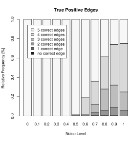
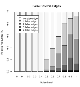
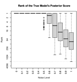
Figure 3: Reliability of the actions graph reconstruction in the presence of noise. The noise level was varied from 0 to 1 in steps of 0.1. For each level of noise, the respective plot shows the statistics over 100 sample NEMs containing 5 edges. Left: The number of true positive edges in the highest scoring NEM. Middle: The number of false positive edges in the highest scoring NEM. Right: The (distribution of the) rank of the posterior score of the true model among all posterior scores.

7.2 Utility of prior knowledge

We test the impact of prior knowledge on the quality of the actions graph reconstruction in two ways. First, a fixed “true” model consisting of $4$ actions, $50$ observables and $5$ edges is constructed, and a noisy ratio matrix is generated from it. The noise level is set to $\alpha=0.7$.

Starting from this matrix, a series of exhaustive searches is carried out. Each time, a prior is generated that either fixes a number of truly present edges as present, or which specifies a number of truly absent edges as absent. The quality of reconstruction is assessed in terms of sensitivity and specificity (regarding only those edges that were not known a priori). Since the quality of reconstruction heavily depends on the true actions graph topology, we average the results over 100 sample runs of this procedure.

The left and middle plot of Fig. 4 show the results of this procedure. The left plot illustrates the reconstruction quality in dependence of the number of a priori known present edges. The middle plot does the same for the inclusion of prior knowledge about absent edges. Both plots show that including prior information considerably increases sensitivity and specificity. In particular, information about present edges helps more than information about missing edges.

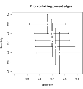
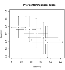
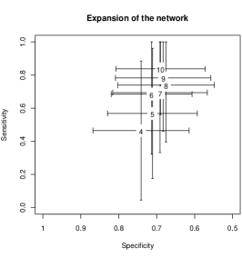
Figure 4: Effects of prior knowledge. Left: Keep a fixed model, and increase the number of known present edges ($0,...,4$). Middle: Keep a fixed model, and increase the number of known absent edges ($0,...,6$). Right: Start with an unknown graph of $4$ actions, and add new actions ($0,...,6$) as well as their adjacent edges to the graph. In all three plots, the error bars range from the first to the third quartile of the distributions obtained in 100 simulation runs.

In a second experiment, a fixed “true” model of $10$ actions and $15$ edges is created, and a noise ratio matrix is generated from it. We randomly pick a subgraph of $4$ actions, the structure of which is assumed to be completely unknown. Another $k$ nodes ($k=0,...,6$) are added to the subgraph, and all edges not belonging to the initial subgraph are correctly specified as known present/absent via the actions graph prior. For each $k$, we restrict the original ratio matrix to the nodes present in the $(k+4)$-nodes subgraph and start an exhaustive search.

Again, the quality of reconstruction is reported by sensitivity and specificity averaged over 100 sample runs. The noise level was set to $0.4$, and the number of observables was set to $200$. The results in the right plot of Fig. 4 show a strong increase in sensitivity at the cost of a slight decrease in specificity.

8 Application to Drosophila immune response

We apply our methodology to data from an RNA interference (RNAi) gene silencing study on innate immune response in Drosophila melanogaster (Boutros et al.,, 2002). The experiment probes how transcriptional response to lipopolysaccharides (LPS) is regulated by signal transduction pathways in the cell.

Data

The data set consists of 16 Affymetrix microarrays: 4 replicates of control experiments without LPS and without RNAi (negative controls), 4 replicates of expression profiling after stimulation with LPS but without RNAi (positive controls), and 2 replicates each of expression profiling after applying LPS and silencing one of the four candidate genes tak, key, rel, and mkk4/hep.

Selectively removing one of these signaling components blocks induction of all, or only parts, of the transcriptional response to LPS. Boutros et al., (2002) show that this observation can be explained by a fork in a signaling pathway below tak, with key and rel on the one side and mkk4/hep on the other. This result clarified the contributions of different pathways to immune response in Drosophila (Royet et al.,, 2005).

Previous analyses

The experimental design of this study, which includes both negative and postive controls, allows to define informative effects of interventions and quantify the false positive and false negative rates. In the original analysis (Boutros et al.,, 2002) and two subsequent studies (Markowetz et al.,, 2005, 2007) only the 68 genes differentially expressed between positive and negative controls were used as effect reporters. Markowetz et al., (2005) propose a simple discretization scheme based on the two controls: if by silencing a gene in the LPS stimulated cell the expression of an LPS-inducible gene moved close to its expression in the negative controls, this was counted as an effect of the intervention; if a gene’s expression stayed close to its expression in the positive controls, the gene was counted as being not affected by the intervention. Applying the same discretization scheme to the positive and negative controls makes it possible to estimate the two error rates.

Analysis based on a single control

The two types of controls can be used to define a set of informative effect reporters and assess the error rates in the data. However, most experimental studies do not contain two kinds of controls but only one. To mimic this situation we will make no use of the negative controls in the dataset and only include the four LPS-induced measurements in our analysis. We show in the following that our improved methodology is still applicable and exploits the information in the data better than previous approaches.

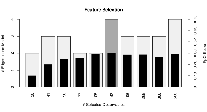
Figure 5: Application of automatic regularization to the Drosophila data set. Each column corresponds to one value of $\delta$ and a selected number of observables between $30$ and $500$. For each value of $\delta$ we plot (1.) the $\operatorname*{PpO}$ score (black bar with scale on the right) and (2.) the number of edges in the inferred model (gray bar with scale on the left). The dark grey bar at $143$ observables indicates the optimal degree of regularization. The corresponding model is discussed in Fig. 6.

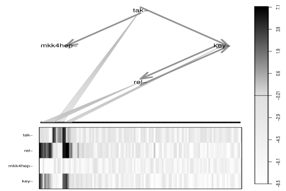
Figure 6: Results on Drosophila data. The upper graph represents $\hat{\Gamma}$ on $\mathcal{A}=\{\text{key-},\text{tak-},\text{rel-},\text{mkk4/hep-}\}$, while the assignment $\hat{\Theta}$ is shown as grey lines connecting nodes in $\hat{\Gamma}$ with observables. The matrix below shows the ratio matrix $R$ (where each column is one observable) with darker values of grey indicating higher likelihood rations (see the colorbar on the right). The graph $\hat{\Gamma}$ places tak above all other nodes and shows a branch below tak with key and rel on one side and mkk4/hep on the other side. The double headed arrow between key and rel shows that the model can not distinguish between them (see the nearly identical rows in the ratio matrix).

Calculation of the ratio matrix $R$

We use well established methods to assess differential gene expression between the positive controls (LPS stimulation but no gene silencing) and the gene perturbation profiles. Because of the small number of samples we chose a highly regularized empirical Bayes method for assessing differential expression in microarray experiments (Smyth,, 2004), which is implemented in the R-package limma (Smyth,, 2005) available from www.bioconductor.org. The empirical Bayes approach is equivalent to shrinkage of the estimated sample variances towards a pooled estimate, resulting in far more stable inference when the number of arrays is small. We compute likelihood ratios for the comparison of positive controls against every gene perturbation. We then select genes which show a positive ratio (regardless of its size) for at least two of the four knock-downs. This simple step of deleting uninformative genes reduces the number of effect reporters (observables) from 14 010 to 904. This number is still much bigger than the number of differential genes used in previous analyses and makes feature selection necessary.

Results

We fit NEM models to the ratio matrix $R$ using the feature selection mechanism described in section 6.2. The resulting curve of the $\operatorname*{PpO}$ statistic is shown in Fig 5. The model selected in our automatic procedure includes 143 observables (out of 904) and is shown in Fig. 6.

Our model places tak above all other nodes and shows a branch below tak with key and rel on one side and mkk4/hep on the other side. The gene perturbations key and rel remain undistinguishable due to almost identical phenotypic profiles (see the nearly identical rows in the ratio matrix in Fig. 6). The branching below tak into two sub-pathways is the main biological feature of the data (Boutros et al.,, 2002) and our model succeeds in recapitulating it.

A previous analysis of the same data set (Markowetz et al.,, 2005) showed a very similar picture but included one additional edge from tak to rel, which is not contained in our result. It is known that rel is a transcription factor responsible for immune response, which is activated via the kinase key (Royet et al.,, 2005). Thus, the additional edge from tak to rel was a spurious result. It can be explained by the fact that the NEMs used in (Markowetz et al.,, 2005) were constrained to transitively closed graphs (and then the direct edge from tak to rel is needed because there is a path from tak to rel over key). This shows that our general formulation of NEMs, which is not constrained to transitively closed graphs, can yield results closer to biological reality than previous formulations.

9 Discussion

In this paper we introduced a generalized definition of Nested Effects Models and expanded their statistical basis in several important directions. Our most important theoretical result is that NEMs can be shown to be identifiable under mild conditions on the data.

General NEMs

The new general formulation of NEMs expands the model class from transitively closed graphs to all directed graphs. This reduces the bias in the model and leads to results closer to existing biological knowledge in the application to Drosophila immune response.

Likelihood formulation

The new likelihood equation is much more flexible than previous equations for binary data (Markowetz et al.,, 2005, 2007). It is applicable to any kind of data by converting it into likelihood ratios for the comparison of effects and non-effects. Thus, it can even integrate heterogeneous sources of data as long as they can be translated into likelihood ratios. Additionally, missing data or the exclusion of bad measurements is possible without changes in the algorithm.

Model search

Our formulation of the likelihood also leads to a fast updating procedure which can be carried out in linear time and is exceedingly faster than previous approaches. Still, an exhaustive search is clearly infeasible for larger values of perturbed genes. However, the fast elementary moves introduced here allow the application of combinatorial search algorithms, like Markov Chain Monte Carlo (Gilks et al.,, 1996) or simulated annealing (Kirkpatrick et al.,, 1983), to find high scoring models.

Prior knowledge

We showed the usefulness of incorporating prior knowledge into model search by fixing parts of a bigger model and only inferring the unknown part. This is a special case of a prior distribution on the space of model graphs. We hope to extend this approach to more flexible structure priors. One promising research direction could be to use a structure prior that favors transitively closed graphs. In this way it would be possible to find a balance between the less biased models introduced here and the causally interpretable but more constrained models introduced earlier (Markowetz et al.,, 2005, 2007).

Availability of software

The NEM exhaustive search algorithm and all its extensions described in this paper are implemented, documented and ready to use in the R package Nessy, which is available at www.bioconductor.org. It includes a plotting routine that conveniently displays nested effects models (see, e.g., Fig 6).

Appendix: Proofs of Theorems

Theorem 1

If the data is consistent with the effects model $F$, then the maximum likelihood estimate of (3) equals $F$,

$$F=\ \underset{G}{\operatorname*{argmax}}\ P(D|G)\ \underset{(\ref{trace1})}{=}\ \underset{G}{\operatorname*{argmax}}\ tr(GR)\ .$$

Proof.

We have $tr(GR)=\sum_{a\in\mathcal{A}}\sum_{s\in\,\mathcal{O}}G_{as}R_{sa}$.

If $F_{as}=1$, then by consistency of the data $R_{sa}>0$ and the choice $G_{as}=1=F_{as}$ maximizes the summand $G_{as}R_{sa}$.

If $F_{as}=0$, then $R_{sa}\leq 0$ and the coice $G_{as}=0=F_{as}$ maximizes the summand $G_{as}R_{sa}$. Hence $\underset{G}{\operatorname*{argmax}}\ tr(GR)=F$. ∎

Lemma 2

Let $(\Gamma^{\prime},\Theta^{\prime})$ be a reversal of $(\Gamma,\Theta)$ induced by the permutation $\pi=(a_{1},a_{2},...,a_{n})$. Then $(\Gamma^{\prime},\Theta^{\prime})$ is a valid parametrization of $F=\Gamma\Theta$ .

Proof.

Let $e_{a}$ denote the $a$-th unit column vector of length $n_{\mathcal{O}}$. Clearly, $\Gamma^{\prime}\Theta^{\prime}=(\Gamma S^{-1})(S\Theta)=\Gamma\Theta=F$. The only additional requirement we need to check is $\Gamma^{\prime}_{aa}=1$ for all $a\in\mathcal{A}$. This holds because of

$$\Gamma^{\prime}_{aa} = e_{a}(\Gamma S^{-1})e_{a}^{T}\;=\;e_{a}\Gamma\sum_{b\in\mathcal{A}}e_{\pi(b)}^{T}e_{b}e_{a}^{T}\;=\;e_{a}\Gamma e_{\pi(a)}^{T}\;=\;$$

$$= \Gamma_{a\pi(a)}\;=\;\begin{cases}\Gamma_{a_{j}\pi(a_{j})}&\text{if }a\in\{a_{1},...,a_{n}\}\\ \Gamma_{aa}&\text{otherwise}\end{cases}\ \;=\;1.$$

∎

Theorem 3

Let $(\Gamma,\Theta)$ and $(\Gamma^{\prime},\Theta^{\prime})$ be the parameters of two nested effects models. Assume that no two distinct actions $a,b\in\mathcal{A}$ have the same parents in $\Gamma$ or in $\Gamma^{\prime}$. Then $(\Gamma,\Theta)$ and $(\Gamma^{\prime},\Theta^{\prime})$ are observationally equivalent if and only if the tuples can be converted one into another by a sequence of disjoint reversals.

Proof.

”$\Leftarrow$”: This follows immediately from Lemma 2.
”$\Rightarrow$”: For an action $a\in\mathcal{A}$, denote the parents of $a$ in $\Gamma$ by $\text{pa}_{\Gamma}(a)=\{b\in\mathcal{A}\,|\,b\stackrel{{\scriptstyle\Gamma}}{{\to}}a\}$. Recall that for an actions graph $\Gamma$, $a\in\text{pa}_{\Gamma}(a)$ for all $a\in\mathcal{A}$. The set of observables attached to $a$ via the effects graph $\Theta$ is called the children of $a$ in $\Theta$, $\text{ch}_{\Theta}(a)=\{s\in\mathcal{O}\,|\,a\stackrel{{\scriptstyle\Theta}}{{\to}}s\}$. Since $\text{pa}_{\Gamma}(a)$ determines $\Gamma_{\cdot a}$ (and vice versa), and $\text{ch}_{\Theta}(a)$ determines $\Theta_{a\cdot}$ (and vice versa), the family of all parents sets determines $\Gamma$ and the family of all children sets determines $\Theta$.
Assume that $\text{ch}_{\Theta}(a)$ and $\text{ch}_{\Theta^{\prime}}(b)$ intersect nontrivially, say $a\stackrel{{\scriptstyle\Theta}}{{\to}}s$, $b\stackrel{{\scriptstyle\Theta^{\prime}}}{{\to}}s$. Then

$$\Gamma_{\cdot a}=\Gamma_{\cdot\theta(s)}=(\Gamma\Theta)_{\cdot s}=(\Gamma^{\prime}\Theta^{\prime})_{\cdot s}=\Gamma^{\prime}_{\cdot\theta^{\prime}(s)}=\Gamma^{\prime}_{\cdot b}$$ (9.1)

Hence

$$\text{pa}_{\Gamma}(a)=\text{pa}_{\Gamma^{\prime}}(b)$$ (9.2)

Furthermore, let $t\in\text{ch}_{\Theta}(a)$ and $t\in\text{ch}_{\Theta^{\prime}}(c)$. Then by (9.2), $\text{pa}_{\Gamma}(a)=\text{pa}_{\Gamma^{\prime}}(c)$, which in turn together with (9.2) implies $\text{pa}_{\Gamma^{\prime}}(b)=\text{pa}_{\Gamma^{\prime}}(c)$. By the hypothesis, this is only possible if $b=c$. Thus $\text{ch}_{\Theta}(a)\subseteq\text{ch}_{\Theta^{\prime}}(b)$, and for symmetric reasons, $\text{ch}_{\Theta}(a)=\text{ch}_{\Theta^{\prime}}(b)$. It follows that the partitions

$$\bigcup_{a\in\mathcal{A}}\hskip 6.25958pt\text{ch}_{\Theta}(a)=\mathcal{O}=\bigcup_{a\in\mathcal{A}}\hskip 6.25958pt\text{ch}_{\Theta^{\prime}}(a)$$ (9.3)

are identical up to order. Therefore there exists a permutation $\pi$ of $\mathcal{A}$ such that

$$\text{ch}_{\Theta^{\prime}}(a)=\text{ch}_{\Theta}(\pi(a))\ \ ,\ a\in\mathcal{A}$$ (9.4)

Together with (9.2) this implies

$$\text{pa}_{\Gamma^{\prime}}(a)=\text{pa}_{\Gamma}(\pi(a))\ \ ,\ a\in\mathcal{A}$$ (9.5)

In other words, $(\Gamma^{\prime},\Theta^{\prime})$ is determined completely by $(\Gamma,\Theta)$ and $\pi$. Let us investigate $\pi$ a little closer. Let $T=\sum_{b\in\mathcal{A}}e_{b}e_{\pi(b)}^{T}$ be the permutation matrix associated with $\pi$. We confirm that

$$(T\Theta)_{a\cdot}=e_{a}^{T}\sum_{b\in\mathcal{A}}e_{b}e_{\pi(b)}^{T}\Theta=e_{\pi(a)}^{T}\Theta=\Theta_{\pi(a)\cdot}\stackrel{{\scriptstyle(\ref{thm.2})}}{{=}}\Theta^{\prime}_{a\cdot}\ \ ,\ a\in\mathcal{A}\ ,$$ (9.6)

so $\Theta^{\prime}=T\Theta$. By analogous calculations, $\Gamma^{\prime}=\Gamma T^{-1}$. Now for $a\in\mathcal{A}$,

$$1=\Gamma^{\prime}_{aa}\stackrel{{\scriptstyle(\ref{thm.3})}}{{=}}\Gamma_{a\pi(a)}\ ,$$ (9.7)

which means that there exists an edge from $a$ to $\pi(a)$ in $\Gamma$. For any $a\in\mathcal{A}$, $\Gamma$ must therefore contain the cycle $a\to\pi(a)\to\pi^{2}(a)\to...\to a$.

Let $\pi=\pi_{1}\pi_{2}\cdot...\cdot\pi_{m}$ be a decomposition of $\pi$ into disjoint cycles, and let $T_{1},T_{2},...,T_{m}$ be the $n_{\mathcal{A}}\times n_{\mathcal{A}}$ permutation matrices corresponding to $\pi_{1},\pi_{2},...,\pi_{m}$ respectively. Clearly, $T=T_{1}T_{2}\cdot...\cdot T_{m}$.

Define $(\Gamma_{0},\Theta_{0})=(\Gamma,\Theta)$, and inductively $(\Gamma_{j},\Theta_{j})=(\Gamma_{j-1}T_{j}^{-1},T_{j}\Theta_{j-1})$, $j=1,...,m$. Then $(\Gamma_{m},\Theta_{m})=(\Gamma T^{-1},T\Theta)=(\Gamma^{\prime},\Theta^{\prime})$, and we have constructed a sequence of disjoint reversals converting $(\Gamma,\Theta)$ into $(\Gamma^{\prime},\Theta^{\prime})$. ∎

References

- Boutros et al., (2002) Boutros, M., Agaisse, H., and Perrimon, N. (2002). Sequential activation of signaling pathways during innate immune responses in Drosophila. Dev Cell, 3(5):711–22.
- Boutros et al., (2004) Boutros, M., Kiger, A. A., Armknecht, S., Kerr, K., Hild, M., Koch, B., Haas, S. A., Consortium, H. F. A., Paro, R., and Perrimon, N. (2004). Genome-Wide RNAi Analysis of Growth and Viability in Drosophila Cells. Science, 303(5659):832–835.
- Brown et al., (2006) Brown, J. A., Sherlock, G., Myers, C. L., Burrows, N. M., Deng, C., Wu, H. I., McCann, K. E., Troyanskaya, O. G., and Brown, J. M. (2006). Global analysis of gene function in yeast by quantitative phenotypic profiling. Mol Syst Biol, 2:2006.0001.
- Driessche et al., (2005) Driessche, N. V., Demsar, J., Booth, E. O., Hill, P., Juvan, P., Zupan, B., Kuspa, A., and Shaulsky, G. (2005). Epistasis analysis with global transcriptional phenotypes. Nat Genet, 37(5):471–7.
- Fire et al., (1998) Fire, A., Xu, S., Montgomery, M. K., Kostas, S. A., Driver, S. E., and Mello, C. C. (1998). Potent and specific genetic interference by double-stranded RNA in caenorhabditis elegans. Nature, 391(6669):806 – 811.
- (6) Fröhlich, H., Fellmann, M., Sültmann, H., Poustka, A., and Beissbarth, T. (2007a). Estimating large-scale signaling networks through nested effects models from intervention effects in microarray data. In Proc. German Conference on Bioinformatics, pages 45–54.
- (7) Fröhlich, H., Fellmann, M., Sültmann, H., Poustka, A., and Beissbarth, T. (2007b). Large scale statistical inference of signaling pathways from rnai and microarray data. BMC Bioinformatics, 8.
- Gesellchen et al., (2005) Gesellchen, V., Kuttenkeuler, D., Steckel, M., Pelte, N., and Boutros, M. (2005). An RNA interference screen identifies Inhibitor of Apoptosis Protein 2 as a regulator of innate immune signalling in Drosophila. EMBO Rep, 6(10):979–84.
- Gilks et al., (1996) Gilks, W. R., Richardson, S., and Spiegelhalter, D. J. (1996). Markov Chain Monte Carlo in Practice. Chapman & Hall/CRC.
- Gunsalus et al., (2004) Gunsalus, K. C., Yueh, W.-C., MacMenamin, P., and Piano, F. (2004). RNAiDB and PhenoBlast: web tools for genome-wide phenotypic mapping projects. Nucleic Acids Res, 32(Database issue):D406–10.
- Hughes et al., (2000) Hughes, T. R., Marton, M. J., Jones, A. R., Roberts, C. J., Stoughton, R., Armour, C. D., Bennett, H. A., Coffey, E., Dai, H., He, Y. D., Kidd, M. J., King, A. M., Meyer, M. R., Slade, D., Lum, P. Y., Stepaniants, S. B., Shoemaker, D. D., Gachotte, D., Chakraburtty, K., Simon, J., Bard, M., and Friend, S. H. (2000). Functional discovery via a compendium of expression profiles. Cell, 102:109–126.
- Kirkpatrick et al., (1983) Kirkpatrick, S., Gelatt, C. D., and Vecchi, M. P. (1983). Optimization by simulated annealing. Science, 220:671–680.
- Knuth, (2005) Knuth, D. (2005). The Art of Computer Programming. Generating all tuples and permutations, volume 4. Addison-Wesley.
- Markowetz et al., (2005) Markowetz, F., Bloch, J., and Spang, R. (2005). Non-transcriptional pathway features reconstructed from secondary effects of RNA interference. Bioinformatics, 21(21):4026–4032.
- Markowetz et al., (2007) Markowetz, F., Kostka, D., Troyanskaya, O. G., and Spang, R. (2007). Nested effects models for high-dimensional phenotyping screens. Bioinformatics, 23(13):i305–i312. (ISMB/ECCB preceedings).
- Markowetz and Spang, (2007) Markowetz, F. and Spang, R. (2007). Inferring cellular networks – a review. BMC Bioinformatics, 8(Suppl 6):S5.
- Ohya et al., (2005) Ohya, Y., Sese, J., Yukawa, M., Sano, F., Nakatani, Y., Saito, T. L., Saka, A., Fukuda, T., Ishihara, S., Oka, S., Suzuki, G., Watanabe, M., Hirata, A., Ohtani, M., Sawai, H., Fraysse, N., Latgé, J.-P., Francois, J. M., Aebi, M., Tanaka, S., Muramatsu, S., Araki, H., Sonoike, K., Nogami, S., and Morishita, S. (2005). High-dimensional and large-scale phenotyping of yeast mutants. Proc Natl Acad Sci U S A, 102(52):19015–20.
- Piano et al., (2002) Piano, F., Schetter, A. J., Morton, D. G., Gunsalus, K. C., Reinke, V., Kim, S. K., and Kemphues, K. J. (2002). Gene clustering based on RNAi phenotypes of ovary-enriched genes in C. elegans. Curr Biol, 12(22):1959–64.
- Raamsdonk et al., (2001) Raamsdonk, L., Teusink, B., Broadhurst, D., Zhang, N., Hayes, A., Walsh, M., Berden, J., Brindle, K., Kell, D., Rowland, J., Westerhoff, H., van Dam, K., and Oliver, S. (2001). A functional genomics strategy that uses metabolome data to reveal the phenotype of silent mutations. Nat Biotechnol, 19(1):45–50.
- Royet et al., (2005) Royet, J., Reichhart, J.-M., and Hoffmann, J. A. (2005). Sensing and signaling during infection in drosophila. Curr Opin Immunol, 17(1):11–17.
- Smyth, (2004) Smyth, G. K. (2004). Linear models and empirical bayes methods for assessing differential expression in microarray experiments. Statistical Applications in Genetics and Molecular Biology, 3(1):Article 3.
- Smyth, (2005) Smyth, G. K. (2005). Limma: linear models for microarray data. In Gentleman, R., Carey, V., Dudoit, S., Irizarry, R., and Huber, W., editors, Bioinformatics and Computational Biology Solutions using R and Bioconductor, pages 397–420. Springer, New York.