Resistivity of inhomogeneous quantum wires

Abstract

We study the effect of electron-electron interactions on the transport in an inhomogeneous quantum wire. We show that contrary to the well-known Luttinger liquid result, non-uniform interactions contribute substantially to the resistance of the wire. In the regime of weakly interacting electrons and moderately low temperatures we find a linear in $T$ resistivity induced by the interactions. We then use the bosonization technique to generalize this result to the case of arbitrarily strong interactions.

Since the first measurements of quantized dc conductance in quantum wires quantized , transport properties of these systems have generated a lot of interest. Theoretically, such one-dimensional conductors cannot be described by the conventional Fermi liquid theory, but rather form a qualitatively different state known as the Luttinger liquid LL-th . Recently several characteristic signatures of the Luttinger liquid state have been reported experimentally in quantum wires nanotube ; LL-exp . Perhaps even more interestingly, a number of experiments show anomalies in the transport properties of these systems in the form of a small structure below the first plateau of quantized conductance thomas2 ; reilly ; thomas1 ; kristensen ; cronenwett ; depicciotto , which are not expected in the Luttinger liquid theory FLleads . The so-called “0.7-structure,” which develops at finite temperature in low-density wires, is an example of such deviations from perfect quantization thomas1 ; kristensen ; cronenwett ; depicciotto . While its precise origin still remains unclear, this feature is most likely related to correlations between electrons, which initiated various attempts to study the effect of interactions on the electronic transport in these devices 7theory ; Kostya ; sushkov .

A number of recent theory papers sushkov ; FLleads studied the model of a quantum wire device in which interactions are present only in a small region of a one-dimensional electron system between two non-interacting leads. If the size of the interacting region does not significantly exceed the Fermi wavelength of the electrons in the wire, the interactions give rise to backscattering of either single electrons or pairs, resulting in significant corrections to the quantized conductance sushkov . On the other hand, if the interaction strength varies smoothly over a long distance, such backscattering processes are expected to be exponentially weak and can be neglected. In this regime a model of non-uniform Luttinger liquid, with parameters gradually varying as a function of position is appropriate. Studies of such a model found no correction to the quantized dc conductance of the wire FLleads . It is thus natural to conclude that inhomogeneities of interacting quantum wires at large scales $d\gg k_{F}^{-1}$ do not affect the dc transport beyond the exponentially small backscattering corrections.

In this paper we show that even at $k_{F}d\gg 1$, when the backscattering processes sushkov can be ignored, the inhomogeneity of the interaction strength in the wire gives rise to a finite resistivity at non-zero temperature.

We start by considering an infinite one-dimensional system of weakly interacting spinless electrons, with quadratic dispersion $\epsilon_{p}=p^{2}/2m$. In this simple model, the electron density $n$ is assumed to be uniform, but the strength of the electron-electron interactions varies along the wire. We describe these inhomogeneous interactions by the potential

$${\cal V}(x,y)=V(x-y)~{}\eta\left(\frac{x+y}{2}\right).$$ (1)

Here $V(x-y)$ is the conventional electron-electron repulsive interaction. Coulombic in nature, it is screened by the nearby gates, and for simplicity we will treat it as a short-range interaction. The non-uniformity of the system is then encoded in the dimensionless function $\eta$, which varies at a length scale $d$, large compared with both the Fermi wavelength and the range of the interaction potential $V(x-y)$.

In order to compute the resistance of the wire, we enforce a dc current $I$ to flow through the system. The electrons in the wire then acquire a drift velocity proportional to this current: $v_{d}=I/ne$. In the reference frame moving along the wire with velocity $v_{d}$ the electronic subsystem is in equilibrium, as pointed out by Pustilnik et al. drag in the context of Coulomb drag between two parallel wires. This equilibrium is characterized by a Fermi energy $\epsilon_{F}$ and a temperature $T$.

When viewed in the stationary reference frame, where the electric current does not vanish, the electrons are no longer in thermodynamic equilibrium. In particular, their occupation probabilities cannot, in general, be expressed as a Fermi function of the energy. However, at $T\ll\epsilon_{F}$ the occupation probabilities of the left- and right-moving states near the Fermi level can still be approximated by Fermi functions, albeit with two different temperatures, $T_{L}$ and $T_{R}$. To show that, we note that the electron energy $\epsilon_{p}$ changes to a different value $\tilde{\epsilon}_{p}$ in the stationary frame. Considering a state $p$ near the right Fermi point $p_{F}$, to first order in $p-p_{F}$, we have

$$\frac{\epsilon_{p}-\epsilon_{F}}{\tilde{\epsilon}_{p}-\tilde{\epsilon}_{F}}=\frac{v_{F}(p-p_{F})}{\tilde{v}_{F}(\tilde{p}-\tilde{p}_{F})}=\frac{v_{F}}{\tilde{v}_{F}},$$

where in the stationary frame $\tilde{v}_{F}=v_{F}+v_{d}$, $\tilde{p}=p+mv_{d}$, $\tilde{p}_{F}=p_{F}+mv_{d}$. Thus, the occupation probability of this state can be expressed in terms of its energy $\tilde{\epsilon}_{p}$ in the stationary frame as

$$\frac{1}{e^{(\epsilon_{p}-\epsilon_{F})/T}+1}=\frac{1}{e^{(\tilde{\epsilon}_{p}-\tilde{\epsilon}_{F})/T_{R}}+1},$$

where $T_{R}=T\tilde{v}_{F}/v_{F}=T(1+v_{d}/v_{F})$. Similarly, for the electrons near the left Fermi point $-p_{F}$ one finds the occupation probability given by the Fermi function with the effective temperature $T_{L}=T(1-v_{d}/v_{F})$.

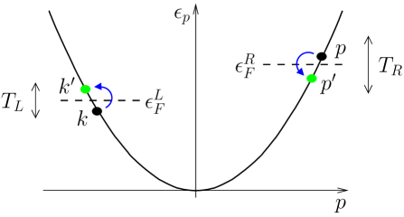
Figure 1: Electronic dispersion in the stationary frame, with an example of non momentum-conserving process. The right- and left-movers Fermi energies read $\epsilon_{F}^{R,L}=\epsilon_{F}(1\pm 2v_{d}/v_{F})$.

One may expect that the electron-electron interactions induce thermalization between right- and left-movers through two-particle scattering processes like the one shown in Fig. 1. In a uniform system, two-particle processes cannot lead to thermalization 3electron because of the conservation of both energy and momentum: the interactions either exchange the momenta of the two electrons or leave them unchanged. However, in our model the non-uniformity of the interaction potential (1) breaks the translational invariance of the system, and allows for two-particle scattering processes that conserve energy but not momentum.

A typical two-particle process shown in Fig. 1 describes the scattering from a state with momenta $(p,k)$ to $(p^{\prime},k^{\prime})$, and is accompanied by an overall loss of momentum. Since this process involves a transfer of energy from the “warmer” right-moving branch to the “colder” left-moving one, it is expected to occur more frequently than the inverse process $(p^{\prime},k^{\prime})\to(p,k)$, so that on average, the two subsystems lose more momentum than they gain. Note that unlike Ref. sushkov, , the typical change of momentum for the processes shown in Fig. 1 is small compared to the Fermi momentum, and the rate of such processes will not become exponentially small at $k_{F}d\gg 1$.

The decrease in momentum can be interpreted as a result of a damping force acting on the electrons. To maintain constant current, it has to be balanced by a driving force, which stems from a local electric field, generated as a response of the system to the current bias drag . Since the damping force is proportional to the temperature difference between the two subsystems, $T_{R}-T_{L}\propto I$, this local electric field is proportional to the applied current, and the proportionality coefficient is defined as the resistivity.

Let us compute the resistivity at temperatures $T\gg\hbar v_{F}/d$. We isolate a small segment of wire taken at position $x$, with the length $\Delta x$ in the range $\hbar v_{F}/T\ll\Delta x\ll d$. The driving force $eE(x)n\Delta x$ acting on this segment of wire as a result of the local electric field $E(x)=\rho(x)I$ compensates for the damping force $\Delta F$ due to the interactions, so that the resistivity can be written as

$$\rho(x)=-\frac{\Delta F}{enI\Delta x}.$$ (2)

We compute the damping force as the change in momentum per unit time, using the Fermi golden rule

$$\Delta F = \frac{2\pi}{\hbar}\sum_{p,k,p^{\prime},k^{\prime}}\left|V_{pk;p^{\prime}k^{\prime}}\right|^{2}\delta(\epsilon_{p}+\epsilon_{k}-\epsilon_{p^{\prime}}-\epsilon_{k^{\prime}})$$ (3)

$$\times\left(p^{\prime}+k^{\prime}-p-k\right)f_{p}^{R}f_{k}^{L}(1-f_{p^{\prime}}^{R})(1-f_{k^{\prime}}^{L}).$$

Here $V_{pk;p^{\prime}k^{\prime}}$ is the matrix element of the interaction potential for scattering from an initial state $(p,k)$ to a final state $(p^{\prime},k^{\prime})$, as shown in Fig. 1, the occupation numbers $f^{R,L}$ are given by the Fermi-Dirac distribution evaluated with the appropriate temperatures $T_{R,L}$. One can easily check that at $T_{R}=T_{L}$ expression (3) vanishes. Then in the linear response regime, one can expand the occupation numbers $f^{R}$ and $f^{L}$ to first order in $T_{R}-T_{L}\propto I$, and find that $\Delta F$ is proportional to the applied current.

To first order in the interaction potential, the matrix element $V_{pk;p^{\prime}k^{\prime}}$ is given by:

$$V_{pk;p^{\prime}k^{\prime}}=\int_{x}^{x+\Delta x}dye^{i\frac{p^{\prime}+k^{\prime}-p-k}{\hbar}y}\left[V(0)-V(2k_{F})\right]\eta(y),$$ (4)

where $V(0)$ and $V(2k_{F})$ are respectively the zero and $2k_{F}$ Fourier components of the interaction potential introduced in Eq. (1). Substituting Eq. (4) into Eq. (3), one readily sees that a constant value of $\eta$ enforces the conservation of momentum and leads to a vanishing result. The dominant non-vanishing part thus involves the gradient of $\eta$, and contributes to $\Delta F$ as $(\partial_{x}\eta)^{2}$.

Performing the remaining momentum summations, the resistivity evaluated to second order in the interaction then takes the form

$$\rho(x)=\frac{h}{64e^{2}}\frac{T}{n\epsilon_{F}}\left(\frac{V(0)-V(2k_{F})}{\pi\hbar v_{F}}\right)^{2}\left(\frac{\partial\eta(x)}{\partial x}\right)^{2}.$$ (5)

This result was obtained in the regime of temperatures $T\gg\hbar v_{F}/d$, for which the position integrals coming from the matrix element (4) could be easily simplified.

Our method provides a clear physical picture of the origin of the resistivity, in the simple case of weakly interacting spinless fermions. We now turn to the case of arbitrarily strong interactions, where we derive the expression for the resistivity using a bosonized Hamiltonian. In addition, we account for electron spins and allow for a non-uniform density $n(x)$, as a result of the surrounding gates and impurities in the substrate.

Following Ref. FLleads, , we generalize the Tomonaga-Luttinger model of interacting one-dimensional electron systems to account for inhomogeneities by allowing for position dependence of the Luttinger-liquid parameters. In the case of electrons with spins, this procedure yields

$$H = H_{\rho}+H_{\sigma}$$ (6a)

$$H_{\rho} = \int dx~{}\frac{\hbar u_{\rho}(x)}{2\pi}\left[K_{\rho}(x)\left(\partial_{x}\theta_{\rho}\right)^{2}+\frac{\left(\partial_{x}\phi_{\rho}\right)^{2}}{K_{\rho}(x)}\right]$$ (6b)

$$H_{\sigma} = \int dx~{}\frac{\hbar u_{\sigma}(x)}{2\pi}\left[K_{\sigma}(x)\left(\partial_{x}\theta_{\sigma}\right)^{2}+\frac{\left(\partial_{x}\phi_{\sigma}\right)^{2}}{K_{\sigma}(x)}\right]$$ (6c)

$$+\int dx~{}\frac{2g_{\sigma}(x)}{\left[2\pi\alpha(x)\right]^{2}}\cos\left(2\sqrt{2}\phi_{\sigma}\right).$$

Here the short distance cutoff $\alpha$ is assumed to be a function of $x$. In the limit of a homogeneous system, $k_{F}d\to\infty$, the coupling constant $g_{\sigma}$ renormalizes to zero at large length scales; at the same time, the parameter $K_{\sigma}$ approaches unity as $K_{\sigma}=1+g_{\sigma}/2\pi\hbar u_{\sigma}$, as required by the SU(2) symmetry LL-th . We assume that $k_{F}d$ is sufficiently large for the system to be near this limit at every point $x$, i.e., $g_{\sigma}(x)/\hbar u_{\sigma}(x)\ll 1$. Previous works on the inhomogeneous Luttinger liquid model were either restricted to spinless electrons FLleads , or discarded ITLL the cosine term in Eq. (6c), invoking the irrelevance of $g_{\sigma}$ at low energies. In our case its contribution to the resistivity is as important as that of the quadratic part of $H_{\sigma}$. In the derivation below, we assume that the inhomogeneities of the system are weak, e.g. $|u_{\rho}(x)-u_{\rho}(0)|\ll u_{\rho}(0)$.

The resistivity can now be computed following a method similar to the one outlined in Ref. Kostya, in the context of a quantum wire in the Wigner crystal regime. As one applies an electric current $I=I_{0}\cos\omega t$, the electrons start moving in the wire. In the dc limit $\omega\to 0$, we can assume that all electrons move in phase, so that at time $t$ their position has shifted by a distance proportional to the injected charge $q(t)=I_{0}\omega^{-1}\sin\omega t$. As a consequence, we need to evaluate all the position-dependent parameters in the Hamiltonian (6) at the true time-dependent position of the electrons, which amounts to replacing $x\to x+q(t)/en(x)$. In the regime of linear response, we only need to expand the Hamiltonian to first order in $q(t)$,

$$H=\int dx\left({\cal H}(x)+\frac{q(t)}{en(x)}{\cal H}^{\prime}(x)\right),$$ (7)

where ${\cal H}(x)$ is the Hamiltonian density when no current is applied, and ${\cal H}^{\prime}(x)$ is obtained from ${\cal H}(x)$ by replacing the position-dependent parameters $g_{\sigma}(x)/\alpha(x)^{2}$, $u_{\nu}(x)K_{\nu}(x)$ and $u_{\nu}(x)/K_{\nu}(x)$ (where $\nu=\rho,\sigma$) by their derivatives with respect to $x$.

In the conventional Luttinger-liquid theory, the current $I=\dot{q}$ is usually viewed as an excitation of the charge mode, and $q(t)$ thus appears as a dynamical variable proportional to $\phi_{\rho}$. Then the linear in $q$ part of Eq. (7) corresponds to cubic terms such as $\phi_{\rho}(\partial_{x}\phi_{\rho})^{2}$. These cubic terms are usually disregarded as irrelevant perturbations to the Luttinger liquid Hamiltonian. Nevertheless, the effect of such perturbations should be addressed, because without them no contribution to transport arises from a non-uniform interaction FLleads . In what follows, it will be more convenient to treat $q(t)$ as an external parameter.

The oscillatory perturbation in the Hamiltonian (7) acts as an external driving force, which leads to the creation of spin and charge excitations and dissipation of the energy from the driving force to the wire. The energy $W$ dissipated into these excitations in unit time may be obtained using the Fermi golden rule. In the limit of weak applied current, it is expected to be quadratic in the amplitude $I_{0}$ of the current oscillations. This allows us, by comparison with the Joule heat law $W=I_{0}^{2}R/2$, to deduce the expression for the resistance $R$ of the wire. Then in the dc limit $\omega\to 0$ we find

$$R=\frac{i}{e^{2}\hbar}\iint\frac{dx\,dy}{n(x)n(y)}\int dt~{}t\,\langle{\cal H}^{\prime}(x,t){\cal H}^{\prime}(y,0)\rangle,$$ (8)

where $\langle\ldots\rangle$ corresponds to the thermodynamic average. The last integral in Eq. (8) falls off rapidly at $|x-y|\gg\hbar u_{\rho,\sigma}/T$. Thus at $T\gg\hbar u_{\rho,\sigma}/d$, we can reduce the expression (8) to a single integral in space, whose integrand we identify with the resistivity $\rho(x)$ of the wire.

As both the charge and spin modes dissipate energy throughout the wire, the total resistivity is given by the sum of a charge and a spin contribution, $\rho(x)=\rho_{\rho}(x)+\rho_{\sigma}(x)$, which can be computed separately. Substituting the charge Hamiltonian (6b) in Eq. (8), and performing the remaining time integral, one can extract the charge contribution to the resistivity

$$\rho_{\rho}(x)=\frac{h}{8\pi e^{2}}\frac{T}{\hbar u_{\rho}(x)[n(x)]^{2}}\left(\frac{\partial_{x}K_{\rho}(x)}{K_{\rho}(x)}\right)^{2}.$$ (9)

This result holds at temperatures in the range $\hbar u_{\rho}/d\ll T\ll D_{\rho}$, where the charge bandwidth $D_{\rho}\sim\hbar nu_{\rho}$.

One can use the expression (9) to recover our earlier result (5) for weakly interacting spinless electrons. In this case, upon bosonization the Hamiltonian of the system takes a form equivalent to $H_{\rho}$ with $u_{\rho}(x)\to v_{F}$ and $K_{\rho}(x)\to 1-\left[V(0)-V(2k_{F})\right]\eta(x)/2\pi\hbar v_{F}$. Substituting these expressions into Eq. (9) and expanding to second order in the interaction, one reproduces the result (5).

The spin contribution to the resistivity consists of two terms arising from substituting the quadratic part and the cosine part of the spin Hamiltonian in Eq. (8). The contribution of the quadratic part of $H_{\sigma}$ can be obtained from Eq. (9) by replacing the charge parameters with their spin counterparts. This result is further simplified by using the low-energy expansion $K_{\sigma}(x)=1+y_{\sigma}(x)/2$, where we introduced the dimensionless parameter $y_{\sigma}(x)=g_{\sigma}(x)/\pi\hbar u_{\sigma}(x)$.

In the case of weakly interacting electrons, the correction to the parameter $K_{\sigma}$ in the quadratic part of Eq. (6c) accounts for the $g_{1}$-coupling of the $z$ components of the electron spins, while the cosine term in $H_{\sigma}$ is associated with the remaining $x$ and $y$ components LL-th . Then from the spin symmetry of the system, the cosine term of the spin Hamiltonian should contribute twice as much to the resistivity as the quadratic part. We expect this result to hold for arbitrarily strong interactions; in the case of weakly interacting electrons, this conclusion can easily be verified unpublished . Combining these two terms, the spin contribution to the resistivity reads:

$$\rho_{\sigma}(x)=\frac{3h}{32\pi e^{2}}\frac{T}{\hbar u_{\sigma}(x)[n(x)]^{2}}[\partial_{x}y_{\sigma}(x)]^{2}.$$ (10)

Again, we restricted ourselves to the range of moderately low temperatures, $\hbar u_{\sigma}/d\ll T\ll D_{\sigma}$, where the spin bandwidth is given by $D_{\sigma}\sim\hbar nu_{\sigma}$.

The comparison of the two contributions (9) and (10) to the resistivity of the wire suggests the strongest effect in the regime of low electron density, when the electron correlations are strong. In this case the exchange coupling $J$ of electron spins, which sets the spin bandwidth $D_{\sigma}$, is strongly suppressed, so that $D_{\sigma}\ll D_{\rho}$. As a result, we expect the spin part (10) of the resistivity to be the dominant contribution in this regime, due to the reduced spin velocity. It is worth pointing out that $y_{\sigma}$ is only marginally irrelevant, so that while it renormalizes to zero at low temperature, it does so logarithmically, as $1/\log(D_{\sigma}/T)$. Furthermore, most experimental measurements are carried out at fixed temperature, while varying the electron density in the wire. In this configuration, the logarithmic dependence of $y_{\sigma}$ suggests that this parameter increases as the interaction in the wire becomes stronger.

Our results are relevant to experiments on wires longer than the length $l_{eq}$ associated with the processes of equilibration in the moving frame. In shorter wires, with length $L\ll l_{eq}$, we expect the resistivity to be suppressed by an additional factor of order $L/l_{eq}$. This raises a fundamental question of the equilibration in a one-dimensional system of interacting electrons. In the weakly interacting case, it is believed that the leading equilibration mechanism is due to three-particle collisions 3electron involving states near the bottom of the electronic band. One expects such processes to be strongly suppressed at low temperatures, corresponding to a large $l_{eq}$. However, such a treatment is not applicable beyond the limit of weak interactions. While we expect stronger interactions to make thermalization easier, a detailed investigation of the equilibration processes will be necessary to access the full temperature dependence of the resistivity in this regime.

In summary, we have shown that the interactions between electrons in a long inhomogeneous quantum wire give rise to a finite resistivity $\rho=\rho_{\rho}+\rho_{\sigma}$, given by Eqs. (9) and (10). This resistivity is due to the weak violation of the momentum conservation in electron-electron collisions, caused by the inhomogeneities on long spatial scales $d\gg k_{F}^{-1}$. Our results can be tested experimentally by measuring the temperature and density dependences of the resistance of long quantum wires.

We are grateful to A. V. Andreev, T. Giamarchi, and L. I. Glazman for helpful discussions. This work was supported by the U.S. Department of Energy, Office of Science, under Contract No. DE-AC02-06CH11357.

References

- (1) B. J. van Wees et al., Phys. Rev. Lett. 60, 848 (1988); D. A. Wharam et al., J. Phys. C 21, L209 (1988).
- (2) See, e.g., T. Giamarchi, Quantum Physics in One Dimension (Clarendon, Oxford, 2004).
- (3) M. Bockrath et al., Nature 397, 598 (1999).
- (4) O. M. Auslaender et al., Science 308, 88 (2005).
- (5) K. J. Thomas et al., Phys. Rev. B 61, R13365 (2000).
- (6) D. J. Reilly et al., Phys. Rev. B 63, 121311(R) (2001).
- (7) K. J. Thomas et al., Phys. Rev. Lett. 77, 135 (1996).
- (8) A. Kristensen et al., Phys. Rev. B 62, 10950 (2000).
- (9) S. M. Cronenwett et al., Phys. Rev. Lett. 88, 226805 (2002).
- (10) R. de Picciotto, L.N. Pfeiffer, K.W. Baldwin and K.W. West, Phys. Rev. B 72, 033319 (2005).
- (11) D. L. Maslov and M. Stone, Phys. Rev. B 52, R5539 (1995); V. V. Ponomarenko, Phys. Rev. B 52, R8666 (1995); I. Safi and H. J. Schulz, Phys. Rev. B 52, R17040 (1995).
- (12) C. K. Wang and K.-F. Berggren, Phys. Rev. B 54, R14257 (1996); B. Spivak and F. Zhou, Phys. Rev. B 61, 16730 (2000); H. Bruus, V.V. Cheianov and K. Flensberg, Physica E 10, 97 (2001); Y. Tokura and A. Khaetskii, Physica E 12, 711 (2002); Y. Meir, K. Hirose and N. S. Wingreen, Phys. Rev. Lett. 89, 196802 (2002); D. Meidan and Y. Oreg, Phys. Rev. B 72, 121312 (2005); O. F. Syljuasen, Phys. Rev. Lett. 98, 166401 (2007).
- (13) K. A. Matveev, Phys. Rev. B 70, 245319 (2004).
- (14) C. Sloggett, A. I. Milstein and O.P. Sushkov, cond-mat/0606649; A. M. Lunde et al., cond-mat/0707.1989.
- (15) M. Pustilnik, E.G. Mishchenko, L.I. Glazman and A.V. Andreev, Phys. Rev. Lett. 91, 126805 (2003).
- (16) A. M. Lunde, K. Flensberg and L. I. Glazman, Phys. Rev. B 75, 245418 (2007).
- (17) I. Safi and H. J. Schulz, Phys. Rev. B 59, 3040 (1999).
- (18) J. Rech and K. A. Matveev (unpublished).