A universal Stein-Tomas restriction estimate for measures in three dimensions

Abstract

We study restriction estimates in ${\mathbb{R}}^{3}$ for surfaces given as graphs of $W^{1}_{1}({\mathbb{R}}^{2})$ (integrable gradient) functions. We obtain a “universal”

$$L^{2}(\mu)\to L^{4}({\mathbb{R}}^{3},L^{2}(SO(3))\,)$$

estimate for the extension operator $f\to\widehat{f\mu}$ in three dimensions. We also prove that the three dimensional estimate holds for any Frostman measure supported on a compact set of Hausdorff dimension greater than two. The approach is geometric and is influenced by a connection with the Falconer distance problem.

1 Introduction

The classical Stein-Tomas restriction theorem says that if $\mu$ is the Lebesgue measure on $S^{d-1}$, the unit sphere in ${\mathbb{R}}^{d}$, or, more generally, on a smooth convex surface with everywhere non-vanishing curvature, then

$${\|\widehat{f\mu}\|}_{L^{\frac{2(d+1)}{d-1}}({\mathbb{R}}^{d})}\lesssim{\|f\|}_{L^{2}(S^{d-1})}.$$ (1.1)

It is shown in [7] (see also [6]) that if the Gaussian curvature is allowed to vanish, (1.1) does not hold. Nevertheless, there is hope of obtaining (1.1) for all reasonable surfaces by modifying the surface carried measure in some universal way. For example, if $\mu_{0}$ is the Lebesgue measure on a convex compact smooth surface $\Gamma$, finite type in the sense that the order of contact with every tangent line is finite, and $d\mu(x)=K^{\frac{1}{d+1}}(x)d\mu_{0}(x)$, then one can check using standard techniques that the estimate (1.1) holds. The situation becomes much more complicated if the Gaussian curvature is allowed to vanish to infinite order. Carbery, Kenig and Ziesler [3] recently proved (1.1) for suitably weighted measures on surfaces of revolution in three dimensions under some quantitative assumption on the graphing function.

In [2], the authors took a different point of view. Instead of imposing a fixed measure on the family of surfaces, they considered mixed norm restriction theorems corresponding to convex curves under rotations. The approach was heavily tied to the average decay estimates of the Fourier transform of the Lebesgue measure on convex curves, due to Podkorytov, which made the convexity assumption difficult to by-pass. In this paper, we take a geometric point of view which allows us to consider a much more general collection of surfaces. Our main result is the following.

Theorem 1.1.

Let $\mu$ be the Frostman measure on a compact $two$-dimensional surface $S$ in ${\mathbb{R}}^{3}$ given as the graph of a $W^{1}_{1}({\mathbb{R}}^{2})$ function. Recall that $W^{1}_{1}({\mathbb{R}}^{2})$ is the class of functions in two variables whose gradient is in $L^{1}({\mathbb{R}}^{2})$.

Given $\theta\in SO(3)$, $d\geq 3$, the special orthogonal group, define the random measure $d\mu_{\theta}$ by the formula

$$\int g(x)\,d\mu_{\theta}(x)=\int f(\theta x)\,d\mu(x).$$

Then,

$${\left(\int{\left|\int_{SO(3)}{|\widehat{f\mu_{\theta}(x)}|}^{2}\,dH(\theta)\right|}^{2}dx\right)}^{\frac{1}{4}}\lesssim{||f||}_{L^{2}(d\mu)},$$ (1.2)

where $dH(\theta)$ is the Haar measure on $SO(3)$.

Moreover, the same estimate holds if $\mu$ is the Frostman measure on any compact subset of ${\mathbb{R}}^{3}$ of Hausdorff dimension greater than two.

Remark 1.2.

The condition we need to impose on the measure $\mu$ in order for the conclusion of Theorem 1.1 to hold is that

$$\mu\times\mu\{(x,y):1\leq|x-y|\leq 1+\epsilon\}\lesssim\epsilon.$$ (1.3)

This condition holds for Lipschitz surfaces, but it also holds for many measures supported on sets that are far from rectifiable in any sense. For example, consider a sequence of positive integers $\{q_{i}\}$ such that $q_{1}=2$ and $q_{i+1}>q_{i}^{i}$. Let $E_{q}$ denote the $q^{-\frac{d}{s}}$, $0<s<d$, neighborhood of $q^{-1}({\mathbb{Z}}^{d}\cap{[0,q]}^{d})$. Let $\displaystyle E_{s}=\cap_{i=1}^{\infty}E_{q_{i}}$. By standard geometric measure theory (see e.g. [4]), the Hausdorff dimension of $E_{s}$ is $s$. Let $s=d-1$. One can check by a direct calculation that (1.3) holds.

1.1 Acknowledgements:

The author wishes to thank Michael Loss of Georgia Institute of Technology for a helpful suggestion regarding the regularity assumptions in the main result. S.R. was partially supported by the NSF grant DMS-0531337.

2 Reduction to the key geometric estimate

Let

$$T(f,g)(x)=\int f\mu_{\theta}*g\mu_{\theta}(x)\,dH_{d}(\theta),$$

where $H$ is the Haar (probability) measure on $SO(d)$.

On one hand,

$${||T(f,g)||}_{L^{1}({\mathbb{R}}^{d})}\lesssim{||f||}_{L^{1}(\mu)}\cdot{||g||}_{L^{1}(\mu)},$$

since convolution of two $L^{1}$ functions is in $L^{1}$ by Fubini.

On the other hand,

$${||T(f,g)||}_{L^{\infty}({\mathbb{R}}^{d})}\lesssim{||f||}_{L^{\infty}(\mu)}\cdot{||g||}_{L^{\infty}(\mu)}\cdot\sup_{x\in{\mathbb{R}}^{d}}\left|\int\mu_{\theta}*\mu_{\theta}(x)\,dx\right|.$$

It follows by interpolation and setting $f=g$ that if

$$\sup_{x\in{\mathbb{R}}^{d}}\left|\int\mu_{\theta}*\mu_{\theta}(x)\,dH(\theta)\right|\lesssim 1,$$ (2.1)

then

$${\left(\int{\left(\int{|\widehat{f\mu_{\theta}}(x)|}^{2}dH_{d}(\theta)\right)}^{2}dx\right)}^{\frac{1}{4}}\lesssim{||f||}_{L^{2}(\mu)}.$$ (2.2)

This reduces matters to the study of (2.1) and this is what the remainder of the paper is about. Since

$$\mathrm{supp}\,(\mu_{\theta}*\mu_{\theta})\subset\mathrm{supp}\,(\mu_{\theta})+\mathrm{supp}\,(\mu_{\theta}),$$

we can easily arrange to take a supremum over $x$ away from a fixed neighborhood of the origin. This is precisely what we shall do in the sequel.

3 Proof of Theorem 1.1

By the Fourier inversion formula

$$\int\mu_{\theta}*\mu_{\theta}(x)\,dH(\theta)$$

$$=\int\int e^{2\pi i\theta x\cdot\xi}{|\widehat{\mu}(\xi)|}^{2}\,dH(\theta)\,d\xi$$

$$=\int\int_{S^{2}}\int_{\{\theta\in SO(3):\theta\frac{x}{|x|}=\omega\}}e^{2\pi i\omega\cdot|x|\xi}\,dH(\theta)\,d\omega{|\widehat{\mu}(\xi)|}^{2}\,d\xi$$

$$=\int\int_{S^{2}}e^{2\pi i\omega\cdot|x|\xi}h(\omega)\,d\omega{|\widehat{\mu}(\xi)|}^{2}\,d\xi,$$ (3.1)

where

$$h(\omega)=H\left(\left\{\theta\in SO(3):\theta\frac{x}{|x|}=\omega\right\}\right).$$

Lemma 3.1.

The function $h(\omega)$ is constant.

The proof is immediate since the Haar measure $dH$ is an invariant probability measure. Since $x$ is fixed, just compose $h$ with the map that takes $\omega$ back to $\frac{x}{|x|}$ and conclude that $h(\omega)=const.$

Going back we see that the expression in (3.1) equals

$$\int\widehat{\sigma}(|x|\xi)\,{|\widehat{\mu}(\xi)|}^{2}\,d\xi$$ (3.2)

$$=\lim_{\epsilon\to 0}\epsilon^{-1}\mu\times\mu\{(u,v):|x|\leq|u-v|\leq|x|(1+\epsilon)\},$$ (3.3)

so the problem reduces to showing that

$$\mu\times\mu\{(u,v):|x|\leq|u-v|\leq|x|(1+\epsilon)\}\lesssim\epsilon.$$ (3.4)

This completes the proof of the three dimensional result, up to (3.4), which takes care of the first part of Theorem 1.1. To prove the second part, observe again that we may assume that $|x|\gtrsim 1$. By the method of stationary phase (see e.g., [8]), we get

$$|\widehat{\sigma}(\xi)|\lesssim{|\xi|}^{-1},$$

and so the expression (3.2) is

$$\lesssim\int{|\xi|}^{-1}{|\widehat{\mu}(\xi)|}^{2}\,d\xi=c\int\int{|x-y|}^{-2}d\mu(x)d\mu(y),$$

which certainly converges if $\mu$ is the Frostman measure on a set of Hausdorff dimension greater than two. This approach just fails to work for two dimensional sets and this is where the $W^{1}_{1}({\mathbb{R}}^{2})$ assumption will play a key role. We now turn to the final section of our paper where this is done.

4 Geometric estimates

In this section we establish (3.4) for measures supported on graphs of $W^{1}_{1}({\mathbb{R}}^{2})$ functions. Assume for a moment that $\mu$ is the Lebesgue measure on a graph of a $C^{1}$ function $G$. We may do that as long as our estimates do not quantitatively depend on this smoothness assumption.

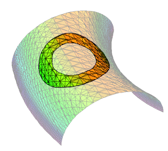
Figure 1: The set $S_{x}$ in the equation (4.1).

We have

$$S_{x}=\{y:1\leq|x-y|\leq 1+\epsilon\}$$ (4.1)

is contained in a curved annulus (see Figure 1) whose dimensions are

$$\epsilon\times\epsilon\times N,$$

where

$$N=\sup_{y,y^{\prime}\in S_{x}}|G(y_{1},y_{2})-G(y^{\prime}_{1},y^{\prime}_{2})|\leq\epsilon\sup_{z\in S_{x}}|\nabla G(z_{1},z_{2})|.$$

If $G$ were Lipschitz, the right hand side above would automatically be bounded by $\epsilon\,C_{Lip}$, independent of $x$, and the proof of (3.4) would be complete. Since we are only assuming that $G$ is in $W^{1}_{1}({\mathbb{R}}^{2})$, we have more work to do. We must show that

$$\int_{\{(x_{1},x_{2}):x\in supp(\mu)\}}\sup_{z\in S_{x}}|\nabla G(z_{1},z_{2})|\,dx_{1}\,dx_{2}\leq C,$$

where $C$ does not depend on smoothness of $G$.

Since the set

$$\{(z_{1},z_{2}):z\in S_{x}\}$$

is contained in a curved $\epsilon\times\epsilon$ square, and we may take $\epsilon$ arbitrarily small, it is enough to show that

$$\int_{\{(x_{1},x_{2}):x\in supp(\mu)\}}|\nabla G(x_{1},x_{2})|dx_{1}dx_{2}\leq C,$$

and this follows instantly from the $W^{1}_{1}({\mathbb{R}}^{2})$ assumption on $G$. This completes the proof.

References

[1]
[2]
L. Brandolini, A. Iosevich, and G. Travaglini,
Spherical means and the restriction phenomenon,
Journal of Fourier Analysis and Applications, 7 (2001), 359-372.
[3] A. Carbery, C. Kenig and S. Ziesler,
Restriction for flat surfaces of revolution on ,
Proc. Amer. Math. Soc., 135 (2007), no. 6, 1905–1914
(electronic).
[4] K. Falconer,
The geometry of fractal sets,
(1985), Cambridge University
Press.
[5] B. J. Green,
Restriction and Kakeya phonomena,
Lecture notes (2003).
[6] A. Iosevich,
Fourier transform, L2 restriction theorem, and scaling,
Bolletino U.M.I., 8 (1999), 383-387.
[7] A. Iosevich and G. Lu,
Sharpness results and Knapp’s homogeneity argument, Bulletin
of the Canad. Math. Bull., 43, (2000), 63-68.
[8] E. M. Stein, Harmonic Analysis,
Princeton University Press, (1993).