Spin-orbit coupling induced interference in quantum corrals

Abstract

Lack of inversion symmetry at a metallic surface can lead to an observable spin-orbit interaction. For certain metal surfaces, such as the Au(111) surface, the experimentally observed spin-orbit coupling results in spin rotation lengths on the order of tens of nanometers, which is the typical length scale associated with quantum corral structures formed on metal surfaces. In this work, multiple scattering theory is used to calculate the local density of states ($LDOS$) of quantum corral structures comprised of nonmagnetic adatoms in the presence of spin-orbit coupling. Contrary to previous theoretical predictions, spin-orbit coupling induced modulations are observed in the theoretical $LDOS$, which should be observable using scanning tunneling microscopy.

In the presence of time reversal symmetry $[E(k,\uparrow)=E(-k,\downarrow)]$ and spatial inversion symmetry $[E(k,\uparrow)=E(-k,\uparrow)]$, no spin splitting can exist since $E(k,\uparrow)=E(k,\downarrow)$. At a metal surface, however, spatial inversion symmetry is violated, and a spin splitting can therefore occur, i.e., $E(k,\uparrow)\neq E(k,\downarrow)$. The spin-orbit coupling in surface states was first observed by LaShell et al.LaShell96 on the Au(111) surface using photoemission spectroscopy. The form of the spin-orbit interaction was found to be similar to the Rashba spin-orbit couplingBychkov84 , which has been heavily studied in semiconductor heterostructures and quantum wells. Additional experimentalNicolay01 ; Henk03 and theoreticalPetersen00 ; Reinert03 ; Bihlmayer06 evidence have confirmed the presence of significant spin-orbit coupling on the Au(111) surface. Although such a spin-splitting should, in principle, occur on all surfaces, the magnitude of the spin splitting depends very strongly on the nature of the surface. For instance, spin-orbit coupling has never been observed on either the Ag(111) or the Cu(111) surfaces. This is due to the fact that the magnitude of the spin-orbit coupling is determined largely by the atomic spin-orbit coupling and the gradient of the surface state wave function at the nucleusBihlmayer06 ; theoretical calculations, which accurately predict the observed spin-orbit coupling on the Au(111) surface, predict the spin-orbit coupling on the Ag(111) to be a factor of 20 smaller than the spin-orbit coupling on the Au(111) surfaceReinert03 ; Bihlmayer06 , well outside the range of current experimental observation. In addition to the Au(111) surface, photoemission experiments have discovered a variety of other metallic systems with spin-orbit coupling, such as on the Bi surfacesKoroteev04 , which exhibit an even larger spin-orbit coupling than that found on Au(111).

Although most experimental observations of spin-orbit coupling in surface states are from photoemission spectroscopy, scanning tunneling microscopy (STM) has been used to observe spin-orbit interference in a magnetic sampleBode03 and in nonmagnetic systems with very strong spin-orbit coupling, such as on the Bi(110) surfacePascual04 and in Bi/Ag(111) and Pb/Ag(111) surface alloysAst07 . However, previous theoretical workPetersen00 has argued that scanning tunneling microscopy (STM) could not be used to observe the spin-orbit coupling in surface states; this argument was based on the assumption that the trajectories which interfere at the site of the STM tip are all one-dimensional in nature. Such trajectories do not undergo any net spin rotation, which results in the same standing wave pattern found in the absence of spin-orbit coupling. While the above argument is certainly true for the case of scattering from a single nonmagnetic adatom, trajectories involving multiple scatterers will undergo a net spin rotation, which will lead to spin-orbit induced modulations of the local density of states ($LDOS$), which should be observable using STM.

Multiple scattering trajectories have been shownHeller94 ; Fiete01 ; Fiete03 to be important in understanding the standing wave patterns observed in the $LDOS$ for step edgesCrommie93 , for quantum corralsCrommie93a formed by placing adatoms atop a noble metal surface, and for quantum mirages generated by a magnetic adatom placed inside a quantum corralManoharan00 ; Fiete01 . Previous experimental work has been conducted for quantum corrals on either the Cu(111) surfaceCrommie93a ; Manoharan00 or on the Ag(111) surfaceKliewer00 , where the neglect of spin-orbit coupling, as stated above, is completely justifiedNicolay01 ; Reinert03 . However, this would not be the case for quantum corrals formed on the Au(111) surface. In this work, multiple scattering theory in the presence of spin-orbit coupling is used to calculate the expected change in the $LDOS$ for quantum corrals formed on surfaces with significant spin-orbit coupling, such as Au(111). Numerical calculations performed for both a circular and a stadium quantum corral formed from nonmagnetic adatoms demonstrate that spin-orbit coupling can lead to observable changes in the $LDOS$. Understanding the effects of spin-orbit induced interference on metal surfaces will be important if such systems are to be used for future spintronics applications.

The effective Hamiltonian for a surface state in the presence of the Rashba spin-orbit interaction is given by:

$$\widehat{H}=\frac{\widehat{P}_{X}^{2}}{2m^{*}}+\frac{\widehat{P}_{Y}^{2}}{2m^{*}}-\frac{\alpha}{\hbar}\left(\widehat{P}_{Y}\widehat{\sigma}_{X}-\widehat{P}_{X}\widehat{\sigma}_{Y}\right)+E_{0}$$ (1)

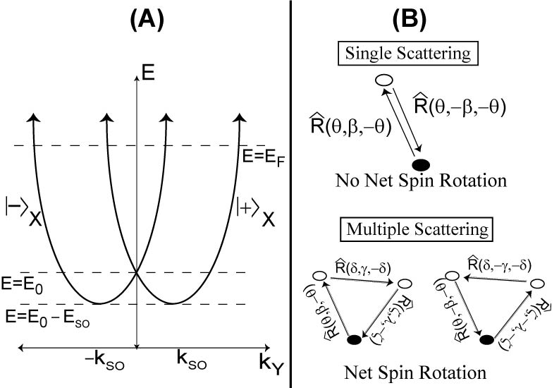
Figure 1: (A) The dispersion curve projected along $k_{X}=0$ in the presence of spin-orbit coupling. The normal parabolic dispersion relation has been split into two parabolic curves, centered about $k_{Y}=\pm k_{\text{SO}}$, with the band edge occurring at an energy of $E_{0}-E_{\text{SO}}$. Note that the spin state is $|+(0)\rangle\equiv|+\rangle_{X}$ for the parabolic band centered at $k_{Y}=+k_{\text{SO}}$ and $|-(0)\rangle\equiv|-\rangle_{X}$ for the parabolic band centered at $k_{Y}=-k_{\text{SO}}$. (B) For a single scattering trajectory, spin-orbit coupling cannot generate a net spin rotation since $\widehat{R}(\theta,\beta,-\theta)\widehat{R}(\theta,-\beta,-\theta)=\widehat{1}$. However, for non-collinear multiple scattering trajectories, a net spin rotation can occur since $\widehat{R}(\theta,\pm\beta,-\theta)\widehat{R}(\delta,\pm\gamma,-\delta)\widehat{R}(\zeta,\pm\lambda,-\zeta)\neq\widehat{1}$.

where $m^{*}$ is the effective mass, $\alpha$ is the spin-orbit coupling strength, and $E_{0}$ is an energy offset arising from the confinement of the electron to the surface. The eigenstates of $\widehat{H}$ with energy $E$ are given by $\Psi_{1}(\vec{r})=\exp(\text{i}\vec{k}_{1}(E)\cdot\vec{r})|+(\phi)\rangle$ and $\Psi_{2}(\vec{r})=\exp(\text{i}\vec{k}_{2}(E)\cdot\vec{r})|-(\phi)\rangle$, where the spin quantization axis for $|\pm(\phi)\rangle$ depends upon the momentum vector, $\vec{k}_{1(2)}(E)=k_{1(2)}(E)\left(\cos(\phi)\widehat{x}+\sin(\phi)\widehat{y}\right)$, where $k_{1}(E)=k_{\text{SO}}+\overline{k}(E)$ and $k_{2}(E)=-k_{\text{SO}}+\overline{k}(E)$, with $k_{\text{SO}}=\frac{m^{*}\alpha}{\hbar^{2}}$ and $\overline{k}(E)=\sqrt{\left(k_{\text{SO}}\right)^{2}+\frac{2m^{*}(E-E_{0})}{\hbar^{2}}}$ (for convenience, the energy dependence of $k_{1}$, $k_{2}$, and $\overline{k}$ will not be explicitly written from now on). For a given value of $\phi$, the spin states are $|\pm(\phi)\rangle=(\sqrt{2})^{-1}\left(|+\rangle_{Z}\pm\exp(-\text{i}\phi)|-\rangle_{Z}\right)$, where $|\pm\rangle_{Z}$ are eigenstates of $\widehat{\sigma}_{Z}$. Due to spin-orbit coupling, the dispersion relation, $E(\vec{k})=\frac{\hbar^{2}|\vec{k}|^{2}}{2m^{*}}\mp\alpha|\vec{k}|+E_{0}$, consists of two parabolic bands centered about $\pm k_{\text{SO}}$ with the bottom of the bands occurring at an energy $E_{0}-E_{\text{SO}}$ (where $E_{\text{SO}}=\frac{\hbar^{2}k^{2}_{\text{SO}}}{2m^{*}}$) instead of at energy $E_{0}$. The dispersion relation is plotted in Figure 1(A) for $k_{X}=0$, where the spin states are $|+(0)\rangle\equiv|+\rangle_{X}$ for the band centered at $k_{Y}=k_{\text{SO}}$ and $|-(0)\rangle\equiv|-\rangle_{X}$ for the band centered at $k_{Y}=-k_{\text{SO}}$. The full two-dimensional dispersion curve in the $k_{X}-k_{Y}$ plane can be found by simply rotating the dispersion curve in Fig. 1(A) using $\exp\left(-\text{i}\theta/\hbar\widehat{L}_{Z}\right)\exp\left(-\text{i}\theta/2\widehat{\sigma}_{Z}\right)$, where $\theta\in[0,\pi)$ and $\widehat{L}_{Z}$ is the $\widehat{z}$-component of the angular momentum operator.

In an STM experimentTersoff85 , the bias voltage between the tip and the surface, $V$, can be changed in order to probe the local density of states at an energy $E_{F}+eV$ (where $E_{F}$ is the Fermi energy of the metal) by measuring the local conductance, $\frac{\text{d}I}{\text{d}V}(E_{F}+eV,\vec{r})$, since $\frac{\text{d}I}{\text{d}V}(E_{F}+eV,\vec{r})\propto LDOS(E_{F}+eV,\vec{r})$ where $LDOS(E,\vec{r})=\sum_{q=\pm}\sum_{\nu}\langle\vec{r},q|\Psi_{\nu}\rangle\langle\Psi_{\nu}|\vec{r},q\rangle\delta(E-E_{\nu})$. Thus in order to calculate the STM image, the $LDOS(E_{F}+eV,\vec{r})$ must be determined. One method of determining the $LDOS(E_{F}+eV,\vec{r})$ is by calculating the Green’s function, $\widehat{G}_{\pm}(\vec{r}_{1},\vec{r}_{2},E_{F}+eV)$, and using the following relationship:

$$LDOS(E_{F}+eV,\vec{r}) = \frac{\text{i}}{2\pi}\text{Trace}_{\text{spin}}\left[\widehat{G}_{+}(\vec{r},\vec{r},E_{F}+eV)-\widehat{G}_{-}(\vec{r},\vec{r},E_{F}+eV)\right]$$ (2)

Thus knowledge of the Green’s function can be used to calculate the expected STM signal.

The free-particle Green’s function in the presence of Rashba spin-orbit coupling and for $E\geq E_{0}-E_{\text{SO}}$ is given byWalls06 ; Csordas06 :

$$\widehat{G}^{0}_{\pm}(\vec{r}_{1},\vec{r}_{2},E) = \mp\text{i}\frac{m^{*}}{4\overline{k}\hbar^{2}}\left(\begin{array}[]{cc}G^{D}_{\pm}(E,r_{12})&\pm\text{i}\exp(\text{i}\theta_{12})G^{S}_{\pm}(E,r_{12})\\ \pm\text{i}\exp(-\text{i}\theta_{12})G^{S}_{\pm}(E,r_{12})&G^{D}_{\pm}(E,r_{12})\end{array}\right)$$ (5)

where $r_{12}=|\vec{r}_{1}-\vec{r}_{2}|$, $\exp(\pm\text{i}\theta_{12})=[(\vec{r}_{1}-\vec{r}_{2})\cdot\widehat{y}\pm\text{i}(\vec{r}_{1}-\vec{r}_{2})\cdot\widehat{x}]/r_{12}$, $G^{D}_{\pm}(E,r_{12})=k_{1}H_{0}^{\pm}(k_{1}r_{12})+k_{2}H_{0}^{\pm}(k_{2}r_{12})$, and $G^{S}_{\pm}(E,r_{12})=k_{1}H^{\pm}_{1}(k_{1}r_{12})-k_{2}H^{\pm}_{1}(k_{2}r_{12})$. Note that $k_{2}\leq 0$ for energies $E_{0}-E_{\text{SO}}\leq E_{F}+eV\leq E_{0}$, so that in this energy range, $H_{n}^{\pm}(k_{2}r_{12})=(-1)^{n+1}H_{n}^{\mp}(|k_{2}|r_{12})$ in Eq. (5). This results in a change in the $LDOS(E_{F}+eV,\vec{r})$ when $E_{0}-E_{\text{SO}}\leq E_{F}+eV\leq E_{0}$: for $E_{F}+eV\geq E_{0}$, the free particle $LDOS_{\text{free}}(E_{F}+eV,\vec{r})$ is independent of energy and is given by $LDOS_{\text{free}}(E_{F}+eV,\vec{r})=m^{*}/(\pi\hbar^{2})$, whereas for $E_{0}-E_{\text{SO}}\leq E_{F}+eV\leq E_{0}$, the $LDOS(E_{F}+eV,\vec{r})$ is dependent upon $E_{F}+eV$ and is given by $LDOS_{\text{free}}(E_{F}+eV,\vec{r})=m^{*}/(\pi\hbar^{2})\times k_{\text{SO}}/\overline{k}$. This change in the $LDOS_{\text{free}}$ has been recently reported for STM measurements on Bi/Ag(111) and Pb/Ag(111) surface alloysAst07 .

In order to gain more physical insight into the transport between $\vec{r}_{1}$ and $\vec{r}_{2}$, $\widehat{G}^{0}_{\pm}(\vec{r}_{1},\vec{r}_{2},E)$ can be rewritten in terms of a complex amplitude multiplied by a “complex” rotation:

$$\widehat{G}^{0}_{\pm}(\vec{r}_{1},\vec{r}_{2},E) = \mp\text{i}\frac{m^{*}}{4\overline{k}\hbar^{2}}bb_{\pm}(E,r_{12})\widehat{R}\left(\frac{\theta_{12}}{2},\pm z_{\pm}(E,r_{12}),-\frac{\theta_{12}}{2}\right)$$ (6)

where $bb_{\pm}(E,r_{12})=\sqrt{[G^{D}_{\pm}(E,r_{12})]^{2}+[G^{S}_{\pm}(E,r_{12})]^{2}}$, $\widehat{R}(\alpha,\beta,\gamma)=\exp(\text{i}\alpha\widehat{\sigma}_{Z})\exp(\text{i}\beta\widehat{\sigma}_{X})\exp(\text{i}\gamma\widehat{\sigma}_{Z})$ is an arbitrary rotation operator with Euler angles $\alpha,\beta,$ and $\gamma$, and $z_{\pm}(E,r_{12})$ is a complex angle which is defined by $\cos[z_{\pm}(E,r_{12})]=G_{\pm}^{D}(E,r_{12})/bb_{\pm}(E,r_{12})$ and $\sin[z_{\pm}(E,r_{12})]=G_{\pm}^{S}(E,r_{12})/bb_{\pm}(E,r_{12})$. Note that for a trajectory which goes from $\vec{r}_{2}$ to $\vec{r}_{1}$ and then back to $\vec{r}_{2}$, no net spin rotation occurs, since $\widehat{G}^{0}_{\pm}(\vec{r}_{2},\vec{r}_{1})\widehat{G}^{0}_{\pm}(\vec{r}_{1},\vec{r}_{2})\propto\left(bb_{\pm}(E,r_{12})\right)^{2}\widehat{R}(\frac{\theta_{12}}{2},\pm z_{\pm}(E,r_{12}),-\frac{\theta_{12}}{2})\widehat{R}(\frac{\theta_{12}}{2},\mp z_{\pm}(E,r_{12}),-\frac{\theta_{12}}{2})=\left(bb_{\pm}(E,r_{12})\right)^{2}\widehat{1}$.

In the presence of multiple adatoms, the total Green’s function can be significantly altered from $\widehat{G}^{0}_{\pm}(\vec{r}_{1},\vec{r}_{2},E)$ due to the interference between the various multiple scattering trajectories. The total Green’s function in the presence of $N$ nonmagnetic adatoms/scatterers can be approximated as:

$$\widehat{G}_{\pm}(\vec{r}_{1},\vec{r}_{2},E) = \widehat{G}_{\pm}^{0}(\vec{r}_{1},\vec{r}_{2},E)+\sum_{j=1}^{N}\widehat{G}_{\pm}^{0}(\vec{r}_{1},\vec{r}_{j},E)\widehat{s}^{\pm}_{j}\widehat{G}_{\pm}(\vec{r}_{j},\vec{r}_{2},E)$$ (7)

where $\widehat{s}^{\pm}_{j}$ is the “s”-wave scattering amplitude, which is given by $\widehat{s}^{\pm}_{j}=\hbar^{2}/m^{*}[\exp(\pm 2\text{i}\delta_{j}(E))-1]\widehat{1}$, with $\delta_{j}(E)$ being the scattering phase shift. In writing Eq. (7), the scattering length of each adatom was assumed to be much smaller than $2\pi/\overline{k}$ (justifying the “s”-wave approximation) and the spin rotation length, $\pi/k_{\text{SO}}$, which allows one to associate the same scattering amplitude for both the $k_{1}$ and $k_{2}$ scattered waves (see for example Eqs. (32)-(33) of Ref. Walls06 ). The unknown values of the Green’s function at each scatterer $n$, $\widehat{G}_{\pm}(\vec{r}_{n},\vec{r}_{2},E)$, can be found by setting $\vec{r}_{1}=\vec{r}_{n}$ to give:

$$\widehat{G}_{\pm}(\vec{r}_{n},\vec{r}_{2},E) = \widehat{G}_{\pm}^{0}(\vec{r}_{n},\vec{r}_{2},E)+\sum_{j\neq n}\widehat{G}_{\pm}^{0}(\vec{r}_{n},\vec{r}_{j},E)\widehat{s}^{\pm}_{j}\widehat{G}_{\pm}(\vec{r}_{j},\vec{r}_{2},E)$$ (8)

This results in a system of $4N$ equations which can be solved via a simple matrix inversion. With knowledge of $\widehat{G}_{\pm}(\vec{r}_{n},\vec{r}_{2},E)$ for each scatterer $n$, the total Green’s function, $\widehat{G}_{\pm}(\vec{r}_{1},\vec{r}_{2},E)$ in Eq. (7), is determined, thus determining the $LDOS$ by using Eq. (2).

Consider first the simple case of a single nonmagnetic adatom placed atop a metal surface at $\vec{r}_{j}$. The total Green’s function in this case is given by:

$$\vec{G}_{\pm}(\vec{r}_{1},\vec{r}_{2},E)=\widehat{G}_{\pm}^{0}(\vec{r}_{1},\vec{r}_{2},E)+s^{\pm}_{j}\widehat{G}^{0}_{\pm}(\vec{r}_{1},\vec{r}_{j},E)\widehat{G}_{\pm}^{0}(\vec{r}_{j},\vec{r}_{2},E)$$ (9)

which results in a change in the $LDOS(E,\vec{r})$ of $\Delta LDOS(E,\vec{r}_{0})=LDOS(E,\vec{r}_{0})-LDOS_{\text{free}}(E,\vec{r}_{0})=\frac{2}{\pi}\left(\frac{m^{*}}{4\overline{k}\hbar^{2}}\right)^{2}\text{Im}\left[s^{+}_{j}(b_{+}(E,r_{0j}))^{2}\right]$, which, for $\overline{k}r_{0j}\gg 1$ can be approximated as:

$$\Delta LDOS(E_{F}+eV,\vec{r}_{0}) = -\frac{\sqrt{k_{1}k_{2}}}{\overline{k}^{2}r_{0j}}\left(\frac{m^{*}}{\pi\hbar^{2}}\right)^{2}\left(\cos(2\overline{k}r_{0j})\text{Re}[s^{+}_{j}]-\sin(2\overline{k}r_{0j})\text{Im}[s^{+}_{j}]\right)$$ (10)

for $E_{F}+eV>E_{0}$, and as:

$$\Delta LDOS(E_{F}+eV,\vec{r}_{0}) = \frac{\sqrt{k_{1}|k_{2}|}}{\overline{k}^{2}r_{0j}}\left(\frac{m^{*}}{\pi\hbar^{2}}\right)^{2}\left(\cos(2\overline{k}r_{0j})\text{Im}[s^{+}_{j}]+\sin(2\overline{k}r_{0j})\text{Re}[s^{+}_{j}]\right)$$ (11)

for $E_{0}-E_{\text{SO}}\leq E_{F}+eV\leq E_{0}$. Therefore, there exists a change in the $\Delta LDOS$ when $E_{0}-E_{\text{SO}}\leq E_{F}+eV\leq E_{0}$ due to spin-orbit coupling, which is similar to the change observed in the $LDOS_{\text{free}}$ described earlierAst07 . For the case of a single nonmagnetic adatom, this change in the $\Delta LDOS$ would be the only way to detect the presence of spin-orbit coupling, since the period of the spatial modulation in the $\Delta LDOS$, $2\overline{k}$, can only be used to determine the effective energy of the surface state electron, $\overline{k}\equiv\sqrt{\frac{2m^{*}E_{\text{eff}}}{\hbar^{2}}}$. Spin-orbit coupling only shifts the effective bottom of the band from $E_{0}$ to $E_{0}-E_{\text{SO}}$, so measurement of $\overline{k}$ cannot, by itself, help to determine the presence or absence of spin-orbit coupling. The physical reason why spin-orbit coupling doesn’t affect the $LDOS$ in the presence of a single adatom is that for single scattering paths returning to the STM tip, no net spin rotation can occur, as shown in Fig. 1(B). This was the reasoning used to argue that STM couldn’t be used to observe spin-orbit coupling for a surface statePetersen00 . However, in the presence of multiple adatoms, mutliple scattering trajectories can generate a net spin rotation (Fig. 1(B)), which allows the spin-orbit coupling to affect the $LDOS$ in a nontrivial manner. As mentioned earlier, such multiple scattering trajectories are important in understanding the observed $LDOS$ in quantum corrals formed atop noble metal surfacesHeller94 ; Fiete01 ; Fiete03 .

For the calculation of the $LDOS$ on the Au(111) surface, the following parameters were usedLaShell96 : $m^{*}=0.26m_{e}$ and $E_{F}-E_{0}=0.41$ eV (Ref. Kevan87 ), a spin-orbit coupling constant of $\alpha=4\times 10^{-11}$ eV-m (which is $10\%$ smaller than the value given in Ref. Henk03 and $21\%$ larger than the value given in Ref. LaShell96 ). These parameters give a Fermi wavelength of $\lambda_{F}=2\pi/\overline{k}=37.4\AA$ and a spin rotation length of $\pi/k_{\text{SO}}=230.5\AA$. It should be noted that this spin rotation length is about an order of magnitude smaller than the attainable spin-rotation lengths in semiconductor heterostructures, which is mainly attributable to the larger effective mass of the surface state electrons.

In the following calculations, all adatoms were modeled as “black-dots”Heller94 where $\delta(E)=\text{i}\infty$ due to inelastic scattering of electrons into the bulkCrampin96 (modifications of the theory for treating the adatom scattering as purely elasticHarbury96 can also be performed too). In the simulations, each nonmagnetic adatom was placed on a hexagonal lattice at a position $\vec{r}=\frac{a}{2}\left(\left(b_{1}+b_{2}\right)\widehat{x}+\sqrt{3}\left(b_{1}-b_{2}\right)\widehat{y}\right)$, where $a=2.885\AA$ for Au(111), and $b_{1}$ and $b_{2}$ are integers chosen to minimize $|\vec{r}-\vec{r}_{\text{d}}|$, where $\vec{r}_{\text{d}}$ is the desired location for each adatom. It should be mentioned that a hexagonal lattice is a simplified model of the actual Au(111) surface, which undergoes a herringbone reconstructionChen98 . Such a reconstruction acts like a superlattice for the surface state electrons and modifies the electron density; however, such a reconstruction has minimal effect on the spin-orbit coupling as has been demonstrated by theoretical calculationsPetersen00 ; Reinert03 ; Bihlmayer06 and is not considered in the following simulations.

In order to illustrate the effect of spin-orbit coupling on the resulting $\Delta LDOS(E,\vec{r})$, simulations with and without spin-orbit coupling were performed at slightly different applied voltages but with the same effective energy, $E_{\text{eff}}$, in order that both simulations gave the same period in the spatial oscillation of the $\Delta LDOS(E_{\text{eff}},\vec{r})$ in the presence of a single adatom, $2\overline{k}=2\sqrt{2m^{*}E_{\text{eff}}/\hbar^{2}}$. For example, if $V$ was the applied voltage used in the simulation in the absence of spin-orbit coupling, then the applied voltage in the presence of spin-orbit coupling, $V^{\prime}$, would be given by $eV^{\prime}=eV-E_{\text{SO}}=eV-2.7$ meV, with $E_{\text{eff}}=E_{F}-E_{0}+eV=E_{F}-E_{0}+eV^{\prime}+E_{\text{SO}}$. In order to consider only the contributions of spin-orbit to the $\Delta LDOS$ arising from multiple scattering trajectories, effective energies, $E_{\text{eff}}\geq E_{\text{SO}}$, were only considered in order to avoid the intrinsic change in the $\Delta LDOS$ when $0\leq E_{\text{eff}}\leq E_{\text{SO}}$. Note that for the case of the Au(111) surface, this intrinsic change in the $\Delta LDOS$ should in any case be unobservable since $E_{\text{SO}}=2.7$ meV is much smaller than the lifetime broadeningAst07 of $18$ meV.

Simulations were first performed on a circular quantum corral of radius $88.7\AA$ comprised of sixty nonmagnetic adatoms placed atop a hexagonal lattice The calculated $\Delta LDOS(E_{\text{eff}},0)$ at the center of the corral is shown in Figure 2(A) as a function of $E_{\text{eff}}$ in the presence (solid curve) and in the absence (dashed curve) of spin-orbit coupling. The $\Delta LDOS(E_{\text{eff}},0)$ without spin-orbit coupling has been shifted down for convenience. A very simple “particle in a box” modelCrommie93a can be used to interpret the $\Delta LDOS(E_{\text{eff}},0)$ in Fig. 2(A): in the absence of spin-orbit coupling and treating the quantum corral as a circular billiard with radius $R=88.7\AA$, the peaks in the $\Delta LDOS(E_{\text{eff}},0)$ mainly occur when $E_{\text{eff}}$ is equal to an eigenenergy of the circular billiard, $E_{\text{eff}}=E_{n}=\frac{\hbar^{2}(k_{n,0})^{2}}{2m^{*}}$ where $k_{n,0}$ is given by the solution to $J_{0}(k_{n,0}R)=0$. This simple model predicts the peak locations in the $\Delta LDOS(E_{\text{eff}},0)$ to within 10 meV for the first four peaks shown in Fig. 2(A).

A similar model can be applied to the case of a circular billiard with spin-orbit coupling. In this case the eigenstates can be written as:

$$\Psi_{n,m}(\vec{r}) \propto \exp(\text{i}m\theta)\left(\begin{array}[]{c}J_{m}(k_{1}^{n,m}|\vec{r}|)-\frac{J_{m}(k_{1}^{n,m}R)}{J_{m}(k_{2}^{n,m}R)}J_{m}(k_{2}^{n,m}|\vec{r}|)\\ -\text{i}\exp(-\text{i}\theta)\left(J_{m-1}(k^{n,m}_{1}|\vec{r}|)+\frac{J_{m}(k_{1}^{n,m}R)}{J_{m}(k_{2}^{n,m}R)}J_{m-1}(k_{2}^{n,m}|\vec{r}|)\right)\end{array}\right)$$ (13)

which have an effective energy (shifted by $-E_{\text{SO}}$ for comparison to the simulations without spin-orbit coupling) given by $E_{\text{eff}}=\hbar^{2}(k^{n,m}_{1}+k^{n,m}_{2})^{2}/(8m^{*})$, which is determined by the condition:

$$J_{m-1}(k^{n,m}_{1}R)J_{m}(k_{2}^{n,m}R)+J_{m}(k^{n,m}_{1}R)J_{m-1}(k^{n,m}_{2}R)=0$$ (14)

The solutions to Eq. (14) which can have nonzero amplitude at the center of the circular billiard, the degenerate states $\Psi_{n,0}(\vec{r})$ and $\Psi_{n,1}(\vec{r})$, essential come in two types of eigenstates. The first type occurs at energies $E_{\text{eff}}^{n}$ which are only about one to two meV smaller in energy than for the eigenstates $J_{0}(k_{n,0}|\vec{r}|)$ in the absence of spin-orbit coupling. These states, although possessing some $J_{1}(k|\vec{r}|)\exp(\pm\text{i}\theta)$ character, are mostly $J_{0}(k|\vec{r}|)$ in character, which leads to large peaks in the $\Delta LDOS(E_{\text{eff}},0)$ at slightly lower energies than the corresponding peaks in the absence of spin-orbit coupling. The second type of eigenstate determined by Eq. (14) occurs at energies in between the aforementioned energies. These eigenstates, which are closely related to the $m=\pm 1$ eigenstates in the absence of spin-orbit coupling, $J_{\pm 1}(\overline{k}_{n}|\vec{r}|)\exp(\pm\text{i}\theta)$, possess a small amount of $J_{0}(k|\vec{r}|)$ character due to spin-orbit coupling, which can lead to new, albeit small, peaks in the $\Delta LDOS(E_{\text{eff}},0)$ at these energies. The small peak in the $\Delta LDOS(E_{\text{eff}}=31\text{meV},0)$ (and more clearly shown in the inset in Fig. 2(A)) corresponds roughly to such an eigenstate, which, for the circular billiard with spin-orbit coupling, has an energy of $E_{\text{eff}}=29.1$ meV.

Besides the small shift in the peaks of the $\Delta LDOS(E_{\text{eff}},0)$ and the small peak at $E_{\text{eff}}=31$ meV, the observed difference in the $\Delta LDOS(E_{\text{eff}},0)$ with and without spin-orbit coupling is relatively small. However, the $\Delta LDOS$ at other places inside the quantum corral can show considerable differences when spin-orbit coupling is included. A slice of the $\Delta LDOS(E_{\text{eff}},\vec{r})$ through the quantum corral is shown in Figs. 2(B) and 2(C) for the (C) second peak in $\Delta LDOS(E_{\text{eff}},0)$ [$E_{\text{eff}}=58.7$ meV (solid curve) and $E_{\text{eff}}=60.4$ meV (dashed curve)]and for the (B) third peak in $\Delta LDOS(E_{\text{eff}},0)$ [$E_{\text{eff}}=144.1$ meV (solid curve) and $E_{\text{eff}}=145.8$ meV (dashed curve)], where the black rectangles centered at $\pm 88.7\AA$ correspond to the positions of the adatoms in the slice. Note that in the simulations, the $\Delta LDOS(E_{\text{eff}},\vec{r})$ is never calculated within $6\AA$ of the adatoms. As the electron bounces around in the corral, it undergoes an effective spin rotation due to spin-orbit coupling, which modulates the interference patterns seen in the quantum corral, resulting in an enhancement (Fig. 2(C)) or a decrease (Fig. 2(B)) in the $\Delta LDOS(E_{\text{eff}},\vec{r})$ near the edges of the corral.

Besides the circular corral, another corral simulated in this work was a 78 adatom stadium billiard of dimensions $141\AA$ by $285\AA$, where the adatoms were again placed atop a hexagonal lattice. Figure 3 gives the $\Delta LDOS(E_{\text{eff}},\vec{r})$ with and without spin-orbit coupling for roughly zero bias voltage between the tip and surface, i.e., $E_{\text{eff}}=410$ meV. Calculations performed at different $E_{\text{eff}}$ gave similar results (data not shown). As for the circular corrals, the $\Delta LDOS(E_{\text{eff}},\vec{r})$ was artificially set to zero within $6\AA$ of each adatom, which makes the adatom positions clearly visible in Fig. 3(A). Although the general structure of the $\Delta LDOS(E_{\text{eff}},\vec{r})$ with and without spin-orbit coupling appears similar, spin-orbit coupling causes additional structure, such as splittings and intensity variations, to appear in the $\Delta LDOS(E_{\text{eff}},\vec{r})$ as is shown in Fig. 3(A). Such spin-orbit induced interference effects can be more clearly seen in Fig. 3(B), which plots a slice of the $\Delta LDOS(E_{\text{eff}},\vec{r})$ through the center of the stadium corral along the long dimension of the corral. As with the circular corral, changes in the amplitude of the $\Delta LDOS(E_{\text{eff}},\vec{r})$ are seen near the adatoms (black rectangles in Fig. 3(B)). However, spin-orbit coupling causes a splitting in the $\Delta LDOS(E_{\text{eff}},\vec{r})$ near the center of the stadium, where the peak to peak distance is roughly $18\AA$. Additional splittings and modulations of $\Delta LDOS(E_{\text{eff}},\vec{r})$ can also be seen in Fig. 3(A). These calculations clearly demonstrate that spin-orbit coupling can generate significant changes to the $\Delta LDOS(E_{\text{eff}},\vec{r})$ in quantum corrals.

In this work, we have examined the effects of spin-orbit coupling on the local density of states for quantum corrals formed atop the Au(111) surface. Changes in the $LDOS(E_{\text{eff}},\vec{r})$ in both circular and stadium corrals indicate that spin-orbit induced interference effects should be visible using STM on the Au(111) surface, contrary to previous theoretical argumentsPetersen00 . The modulations in the $LDOS(E_{\text{eff}},\vec{r})$ were a result of non-collinear multiple scattering trajectories, such as those found in quantum corrals, which can generate an effective spin-rotation in the presence of spin-orbit coupling. Since the previous experimental data on quantum corrals is quite good and can be accurately described by multiple scattering theoryHeller94 ; Fiete03 , the predicted spin-orbit induced interference in such systems should also be experimentally observable. Furthermore, this work can also be extended to the case of quantum corrals comprised of magnetic adatoms, where, through the spin-orbit coupling of the surface state electronsHeide07 , effective interactions between the magnetic adatoms can be generated. The methodology in this paper can also be used to calculate the $LDOS$ for superlattices formed from localized structures. In the future, ab initio calculations of STM images in quantum corralsStepanyuk05 with spin-orbit coupling will be performed, in addition to examining the effect of the herringbone reconstruction on the resulting $LDOS$ in quantum corrals on Au(111).

JDW would like to thank Prof. Yung-Ya Lin for his support. This work was supported by NSF NSEC.

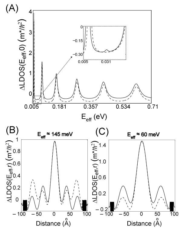
Figure 2: The $\Delta LDOS(E,\vec{r})$ for a circular quantum of radius $88.7\AA$ comprised of 60 nonmagnetic adatoms, which are modeled as “black-dot” scatterers ($\delta(E)=\text{i}\infty$). In (A), the $\Delta LDOS(E_{\text{eff}},0)$ is plotted at the center of the corral as a function of the effective energy, $E_{\text{eff}}$, with (solid curve) and without (dashed curve) spin-orbit coupling. The dashed curve has been shifted downward for convenience. Note that $E_{\text{eff}}$ can be converted into a bias voltage by using either $-eV=E_{F}-E_{0}-E_{\text{eff}}\,\text{(dashed curve)}$ or $-eV^{\prime}=E_{F}-E_{0}+E_{\text{SO}}-E_{\text{eff}}=E_{F}-E_{0}-E_{\text{eff}}+2.7$ meV (solid curve), where $E_{F}-E_{0}=410$ meV for the Au(111) surface. The following parameters were used in the simulation: $m^{*}=0.26m_{e}$ and $\alpha=4\times 10^{-11}$ eV-m. The peaks in the $\Delta LDOS(E_{\text{eff}},0)$ occur when $E_{\text{eff}}$ roughly corresponds to eigenergy for a circular billiard with (solid curve) and without (dashed curve) spin-orbit coupling. A small peak (shown in the inset) in the $\Delta LDOS(E_{\text{eff}},0)$ at $E_{\text{eff}}\approx 31$ meV, corresponds to an eigenstate of the circular billiard with spin-orbit coupling which is mostly $J_{1}(k|\vec{r}|)\exp(\pm\text{i}\theta)$ in character, but, due to spin-orbit coupling, does contain some $J_{0}(k|\vec{r}|)$ character, which can contribute to the $\Delta LDOS(E_{\text{eff}},0)$. In (B) and (C), profiles of the $\Delta LDOS(E_{\text{eff}},\vec{r})$ through the quantum corral (the adatoms are denoted by the black rectangles) with (solid curve) and without (dashed curve) spin-orbit coupling for (C) the second main peak in the $\Delta LDOS(E_{\text{eff}},0)$ [$E_{\text{eff}}=60.4$ meV (without spin-orbit coupling) and $E_{\text{eff}}=58.7$ meV (with spin-orbit coupling)] and for (B) the third main peak in the $\Delta LDOS(E_{\text{eff}},0)$ [$E_{\text{eff}}=145.8$ meV (without spin-orbit coupling) and $E_{\text{eff}}=144.1$ meV (with spin-orbit coupling)]. In both cases, substantial differences in the intensity of the $\Delta LDOS(E_{\text{eff}},\vec{r})$ are observed, where the presence of spin-orbit coupling can either enhance the $\Delta LDOS(E_{\text{eff}},\vec{r})$ (Fig. 2(C)) or decrease the $\Delta LDOS(E_{\text{eff}},\vec{r})$ (Fig. 2(B)).

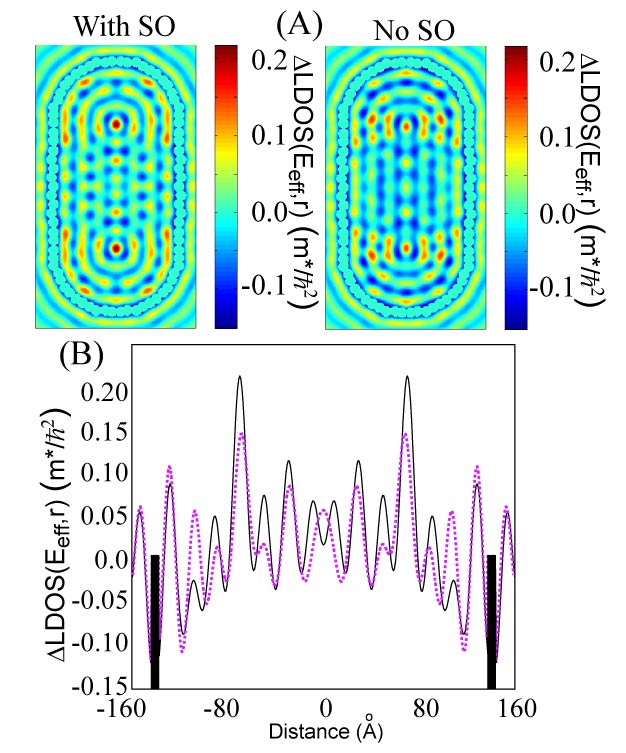
Figure 3: (Color online) Simulation of the $\Delta LDOS(E_{\text{eff}},\vec{r})$ for a 78 adatom quantum corral stadium billiard of width $141\AA$ and length $285\AA$ at $E_{\text{eff}}=410$ meV, with (left) and without (right) spin-orbit coupling. Although the general features are similar, inclusion of spin-orbit coupling can enhance or diminish features in the $\Delta LDOS$ along with introducing additional peaks in the $\Delta LDOS$. This can be more clearly seen in (B), where a slice through the center of the stadium along its long dimension has been plotted with spin-orbit (solid curve) and without (purple dashed curve) spin-orbit coupling. The black rectangles indicate the locations of the adatoms through the slice. Besides differences in peak intensity, a splitting of the $\Delta LDOS$ occurs at the center of the stadium with spin-orbit coupling (peak to peak distance of $\approx 18\AA$, which is absent when spin-orbit coupling is not included.

References

(1)
S. LaShell, B.A. McDougall, and E. Jensen, Phys. Rev. Lett. 77, 3419
(1996).
(2)
Y.A. Bychkov and E.I. Rashba, J. Phys. C 17, 6039 (1984).
(3)
G. Nicolay, F. Reinert, S. Hufner, and P. Blaha, Phys. Rev. B 65, 033407
(2001).
(4)
J. Henk, A. Ernst, and P. Bruno, Phys. Rev. B 68, 165416
(2003).
(5)
L. Petersen and P. Hedegard, Surf. Sci. 459, 49 (2000).
(6)
F. Reinert, J. Phys.: Condens. Matter 15, S693 (2003).
(7)
G. Bihlmayer, Yu.M. Koroteev, P.M. Echenique, E.V. Chulkov, and S.
Blugel,
Surf. Sci. 600, 3888 (2006).
(8)
Yu.M. Koroteev, G. Bihlmayer, J.E. Gayone, E.V. Chulkov, S. Blugel,
P.M.
Echenique, and Ph. Hofmann, Phys. Rev. Lett. 93, 046403 (2004).
(9)
M. Bode, A. Kubetzka, S. Heinze, O. Pietzsch, R. Wiesendanger, M.
Heide, X.
Nie, G. Bihlmayer, and S. Blugel, J. Phys.: Condens. Matter 15, S679
(2003).
(10)
J.I. Pascual, G. Bihlmayer, Yu.M. Koroteev, H.-P. Rust, G. Ceballos,
M.
Hansmann, K. Horn, E.V. Chulkov, S. Blugel, P.M. Echenique, and Ph. Hofmann,
Phys. Rev. Lett. 93, 196802 (2004).
(11)
C.R. Ast, G. Wittich, P. Wahl, R. Vogelgesang, D. Pacile, M.C.
Falub, L.
Moreschini, M. Papagno, M. Grioni, and K. Kern, Phys. Rev. B 75,
201401(R) (2007).
(12)
E.J. Heller, M.F. Crommie, C.P. Lutz, and D.M. Eigler, Nature 369, 464
(1994).
(13)
G.A. Fiete, J.S. Hersch, E.J. Heller, H.C. Manoharan, C.P. Lutz, and
D.M.
Eigler, Phys. Rev. Lett. 86, 2392 .
(14)
G.A. Fiete and E.J. Heller, Rev. Mod. Phys. 75, 934 (2003).
(15)
M.F. Crommie, C.P. Lutz, and D.M. Eigler, Nature 363, 524
(1993).
(16)
M.F. Crommie, C.P. Lutz, and D.M. Eigler, Science 262, 218
(1993).