Unsaturated Throughput Analysis of IEEE 802.11 in Presence of Non Ideal Transmission Channel and Capture Effects

Abstract

In this paper, we provide a throughput analysis of the IEEE 802.11 protocol at the data link layer in non-saturated traffic conditions taking into account the impact of both transmission channel and capture effects in Rayleigh fading environment. The impact of both non-ideal channel and capture become important in terms of the actual observed throughput in typical network conditions whereby traffic is mainly unsaturated, especially in an environment of high interference.

We extend the multi-dimensional Markovian state transition model characterizing the behavior at the MAC layer by including transmission states that account for packet transmission failures due to errors caused by propagation through the channel, along with a state characterizing the system when there are no packets to be transmitted in the buffer of a station. Finally, we derive a linear model of the throughput along with its interval of validity.

Simulation results closely match the theoretical derivations confirming the effectiveness of the proposed model.

I Introduction

Wireless Local Area Networks (WLANs) using the IEEE802.11 series of standards have experienced an exponential growth in the recent past [1-23]. The Medium Access Control (MAC) layer of many wireless protocols resemble that of IEEE802.11. Hence, while we focus on this protocol, it is evident that the results easily extend to other protocols with similar MAC layer operation.

The IEEE802.11 MAC presents two options [1], namely the Distributed Coordination Function (DCF) and the Point Coordination Function (PCF). PCF is generally a complex access method that can be implemented in an infrastructure network. DCF is similar to Carrier Sense Multiple Access with Collision Avoidance (CSMA/CA) and is the focus of this paper.

With this background, let us provide a quick survey of the recent literature related to the problem addressed here. This survey is by no means exhaustive and is meant to simply provide a sampling of the literature in this fertile area. We invite the interested readers to refer to the references we provide in the following and references therein.

The most relevant works to what is presented here are [13, 14, 15]. In [13] the author provided an analysis of the saturation throughput of the basic 802.11 protocol assuming a two dimensional Markov model at the MAC layer, while in [14] the authors extended the underlying model in order to consider unsaturated traffic conditions by introducing a new idle state, not present in the original Bianchi’s model, accounting for the case in which the station buffer is empty, after a successful completion of a packet transmission. In the modified model, however, a packet is discarded after $m$ backoff stages, while in Bianchi’s model, the station keeps iterating in the $m$-th backoff stage until the packet gets successfully transmitted. In [15], authors propose a novel Markov model for the DCF of IEEE 802.11, using a IEEE 802.11a PHY, in a scenario with various stations contending for the channel and transmitting with different transmission rates. An admission control mechanism is also proposed for maximizing the throughput while guaranteeing fairness to the involved transmitting stations.

In [16], the authors extend the work of Bianchi to multiple queues with different contention characteristics in the 802.11e variant of the standard with provisions of QoS. In [17], the authors present an analytical model, in which most new features of the Enhanced Distributed Channel Access (EDCA) in 802.11e such as virtual collision, different arbitration interframe spaces (AIFS), and different contention windows are taken into account. Based on the model, the throughput performance of differentiated service traffic is analyzed and a recursive method capable of calculating the mean access delay is presented. Both articles referenced assume the transmission channel to be ideal.

In [18], the authors look at the impact of channel induced errors and the received SNR on the achievable throughput in a system with rate adaptation whereby the transmission rate of the terminal is adapted based on either direct or indirect measurements of the link quality. In [19], the authors deal with the extension of Bianchi’s Markov model in order to account for channel errors. In [20], the authors investigate the saturation throughput in both congested and error-prone Gaussian channel, by proposing a simple and accurate analytical model of the behaviour of the DCF at the MAC layer. The PHY-layer is based on the parameters of the IEEE 802.11a protocol.

Paper [21] proposes an extension of the Bianchi’s model considering a new state for each backoff stage accounting for the absence of new packets to be transmitted, i.e., in unloaded traffic conditions.

In real networks, traffic is mostly unsaturated, so it is important to derive a model accounting for practical network operations. In this paper, we extend the previous works on the subject by looking at all the three issues outlined before together, namely real channel conditions, unsaturated traffic, and capture effects. Our assumptions are essentially similar to those of Bianchi [13] with the exception that we do assume the presence of both channel induced errors and capture effects due to the transmission over a Rayleigh fading channel. As a reference standard, we use network parameters belonging to the IEEE802.11b protocol, even though the proposed mathematical models hold for any flavor of the IEEE802.11 family or other wireless protocols with similar MAC layer functionality. We also demonstrate that the behavior of the throughput versus the packet rate, $\lambda$, is a linear function of $\lambda$ up to a critical packet rate, $\lambda_{c}$, above which throughput enters saturated conditions. Furthermore, in the linear region, the slope of the throughput depends only on the average packet length and on the number of contending stations.

Paper outline is as follows. After a brief review of the functionalities of the contention window procedure at MAC layer, section II extends the Markov model initially proposed by Bianchi, presenting modifications that account for transmission errors and capture effects over Rayleigh fading channels employing the 2-way handshaking technique in unsaturated traffic conditions. Section III provides an expression for the unsaturated throughput of the link. In section IV we present simulation results where typical MAC layer parameters for IEEE802.11b are used to obtain throughput values as a function of various system level parameters, capture probability, and SNR under typical traffic conditions. Section V derives a linear model of the throughput along with its interval of validity. Finally, Section VI is devoted to conclusions.

II Development of the Markov Model

In this section, we present the basic rationales of the proposed bi-dimensional Markov model useful for evaluating the throughput of the DCF under unsaturated traffic conditions. We make the following assumptions: the number of terminals is finite, channel is prone to errors, capture in Rayleigh fading transmission scenario can occur, and packet transmission is based on the 2-way handshaking access mechanism. For conciseness, we will limit our presentation to the ideas needed for developing the proposed model. The interested readers can refer to [1, 13] for many details on the operating functionalities of the DCF.

II-A Markovian Model Characterizing the MAC Layer under unsaturated traffic conditions, Real Transmission Channel and Capture Effects

In [13], an analytical model is presented for the computation of the throughput of a WLAN using the IEEE 802.11 DCF under ideal channel conditions. By virtue of the strategy employed for reducing the collision probability of the packets transmitted from the stations attempting to access the channel simultaneously, a random process $b(t)$ is used to represent the backoff counter of a given station. Backoff counter is decremented at the start of every idle backoff slot and when it reaches zero, the station transmits and a new value for $b(t)$ is set.

The value of $b(t)$ after each transmission depends on the size of the contention window from which it is drawn. Therefore it depends on the stations’ transmission history, rendering it a non-Markovian process. To overcome this problem and get to the definition of a Markovian process, a second process $s(t)$ is defined representing the size of the contention window from which $b(t)$ is drawn, $(W_{i}=2^{i}W,~{}i=s(t))$.

We recall that a backoff time counter is initialized depending on the number of failed transmissions for the transmitted packet. It is chosen in the range $[0,W_{i}-1]$ following a uniform distribution, where $W_{i}$ is the contention window at the backoff stage $i$. At the first transmission attempt (i.e., for $i=0$), the contention window size is set equal to a minimum value $W_{0}=W$, and the process $s(t)$ takes on the value $s(t)=i=0$.

The backoff stage $i$ is incremented in unitary steps after each unsuccessful transmission up to the maximum value $m$, while the contention window is doubled at each stage up to the maximum value $CW_{max}=2^{m}W$.

The backoff time counter is decremented as long as the channel is sensed idle and stopped when a transmission is detected. The station transmits when the backoff time counter reaches zero.

A two-dimensional Markov process $(s(t),b(t))$ can now be defined, based on two assertions:

1. the probability $\tau$ that a station will attempt transmission in a generic time slot is constant across all time slots;

2. the probability $P_{col}$ that any transmission experiences a collision is constant and independent of the number of collisions already suffered.

Bianchi’s model relies on the following fundamental assumptions: 1) the mobile stations always have something to transmit (i.e., the saturation condition), 2) there are no hidden terminals and there is no capture effect (i.e., a terminal which perceives a higher signal-to-noise ratio (SNR) relative to other terminals capturing the channel [22, 23, 24] and limiting access to other terminals, similar to the near-far problem in cellular networks), 3) at each transmission attempt and regardless of the number of retransmissions suffered, each packet collides with constant and independent probability, and 4) the transmission channel is ideal and packet errors are only due to collisions. Clearly, the first, the second and fourth assumptions are not valid in any real setting, specially when there is mobility and when the transmission channel suffers from fading effects.

The main aim of this section is to propose an effective modification of the bi-dimensional Markov process proposed in [13] in order to account for unsaturated traffic conditions, channel error propagation and capture effects over a Rayleigh fading channel under the hypothesis of employing a 2-way handshaking access mechanism.

It is useful to briefly recall the 2-way handshaking mechanism. A station that wants to transmit a packet, waits until the channel is sensed idle for a Distributed InterFrame Space (DIFS), follows the backoff rules and then transmits a packet. After the successful reception of a data frame, the receiver sends an ACK frame to the transmitter. Only upon a correct ACK frame reception, the transmitter assumes successful delivery of the corresponding data frame. If an ACK frame is received in error or if no ACK frame is received, due possibly to an erroneous reception of the preceding data frame, the transmitter will contend again for the medium.

On the basis of this assumption, collisions can occur with probability $P_{col}$ on the transmitted packets, while transmission errors due to the channel, can occur with probability $P_{e}$. We assume that collisions and transmission error events are statistically independent. In this scenario, a packet is successfully transmitted if there is no collision (this event has probability $1-P_{col}$) and the packet encounters no channel errors during transmission (this event has probability $1-P_{e}$). The probability of successful transmission is therefore equal to $(1-P_{e})(1-P_{col})$, from which we can set an equivalent probability of failed transmission as $P_{eq}=P_{e}+P_{col}-P_{e}P_{col}$.

Furthermore, in mobile radio environment, it may happen that the channel is captured by a station whose power level is stronger than other stations transmitting at the same time. This may be due to relative distances and/or channel conditions for each user and may happen whether or not the terminals exercise power control. Capture effect often reduces the collision probability on the channel since the stations whose power level at the receiver are very low due to path attenuation, shadowing and fading, are considered as interferers at the access point (AP) raising the noise floor.

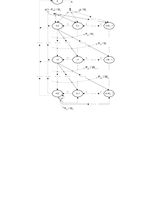
Figure 1: Markov chain for the contention model in unsaturated traffic conditions, based on the 2-way handshaking technique, considering the effects of capture and channel induced errors.

To simplify the analysis, we make the assumption that the impact of the channel induced errors on the packet headers are negligible because of their short length with respect to the data payload size. This is justified on the basis of the assumption that the bit errors affecting the transmitted data are independent of each other. Hence, the packet or frame error rate, identified respectively with the acronyms PER or FER, is a function of the packet length, with shorter packets having exponentially smaller probability of error compared to longer packets.

Practical networks operate in unsaturated traffic conditions. In this case, Bianchi’s model [13] assuming the presence of a packet to be transmitted in each and every station’s buffer, is not valid anymore. However, the simplicity of such a model can be retained also in unsaturated conditions by introducing a new state, labelled $I$, accounting for the following two situations:

• immediately after a successful transmission, the buffer of the transmitting station is empty;

• the station is in an idle state with an empty buffer until a new packet arrives at the buffer for transmission.

With these considerations in mind, let us discuss the Markov model shown in Fig. 1, modelling unsaturated traffic condition. Notice that in our Markov chain we do not model the 802.11 post-backoff feature. However, post-backoff has negligible effects on the theoretical results developed in the paper as exemplified by the simulation results obtained in the following. Similar to the model in [13], $(m+1)$ different backoff stages are considered (this includes the zero-th stage). The maximum contention windows (CW) size is $CWmax=2^{m}W$, and the notation $W_{i}=2^{i}W$ is used to define the $i^{th}$ contention window size. A packet transmission is attempted only in the $(i,0)$ states, $\forall i=0,\ldots,m$. If collision occurs, or transmission is unsuccessful due to channel errors, the backoff stage is incremented, so that the new state can be $(i+1,k)$ with probability $P_{eq}/W_{i+1}$, since a uniform distribution between the states in the same backoff stage is assumed. We consider capture as a subset of the event of a collision (i.e., capture implicitly implies a collision). In other word, the capture event can happen in the presence of collision by allowing the transmitting station with the highest received power level at the access point to capture the channel. In the event of capture, no collision is detected and the Markov model transits into one of the transmitting states $(i,0)$ depending on the current contention stage. If no collision occurs (or is detected), a data frame can be transmitted and the transmitting station enters state $(i,0)$ based on its backoff stage. From state $(i,0)$ the transmitting station re-enters the initial backoff stage $i=0$ if the transmission is successful and at least one packet is present in the buffer, otherwise the station transit in the state labelled $I$ waiting for a new packet arrival. Otherwise, if errors occur during transmission, the ACK packet is not sent, an ACK-timeout occurs, and the backoff stage is changed to $(i+1,k)$ with probability $P_{eq}/W_{i+1}$.

The Markov Process of Fig. 1 is governed by the following transition probabilities:

$$\small\begin{array}[]{lll}P_{i,k|i,k+1}&=1,&~{}k\in[0,W_{i}-2],~{}i\in[0,m]\\ P_{0,k|i,0}&=q(1-P_{eq})/W_{0},&~{}k\in[0,W_{0}-1],~{}i\in[0,m]\\ P_{i,k|i-1,0}&=P_{eq}/W_{i},&~{}k\in[0,W_{i}-1],~{}i\in[1,m]\\ P_{m,k|m,0}&=P_{eq}/W_{m},&~{}k\in[0,W_{m}-1]\\ P_{I|i,0}&=(1-q)(1-P_{eq}),&~{}i\in[0,m]\\ P_{0,k|I}&=q/W_{0},&~{}k\in[0,W_{0}-1]\\ P_{I|I}&=1-q&\end{array}$$ (1)

The first equation in (1) states that, at the beginning of each slot time, the backoff time is decremented. The second equation accounts for the fact that after a successful transmission, a new packet transmission starts with backoff stage 0 with probability $q$, in case there is a new packet in the buffer to be transmitted. Third and fourth equations deal with unsuccessful transmissions and the need to reschedule a new contention stage. The fifth equation deals with the practical situation in which after a successful transmission, the buffer of the station is empty, and as a consequence, the station transits in the idle state $I$ waiting for a new packet arrival. The sixth equation models the situation in which a new packet arrives in the station buffer, and a new backoff procedure is scheduled. Finally, the seventh equation models the situation in which there are no packets to be transmitted and the station is in the idle state.

III Markovian Process Analysis and Throughput Computation

Next line of pursuit consists in finding a solution of the stationary distribution:

$$b_{i,k}=\lim_{t\rightarrow\infty}P[s(t)=i,b(t)=k],~{}\forall k\in[0,W_{i}-1],~{}\forall i\in[0,m]$$

that is, the probability of a station occupying a given state at any discrete time slot.

First, we note the following relations:

$$\begin{array}[]{rcll}b_{i,0}&=&P_{eq}\cdot b_{i-1,0}=P_{eq}^{i}\cdot b_{0,0},&\forall i\in[1,m-1]\\ b_{m,0}&=&\frac{P_{eq}^{m}}{1-P_{eq}}\cdot b_{0,0},&i=m\\ \end{array}$$ (2)

whereby, $P_{eq}$ is the equivalent probability of failed transmission, that takes into account the need for a new contention due to either packet collision ($P_{col}$) or channel errors ($P_{e}$), i.e.,

$$P_{eq}=P_{col}+P_{e}-P_{e}\cdot P_{col}$$ (3)

State $b_{I}$ in Fig. 1 considers both the situation in which after a successful transmission there are no packets to be transmitted, and the situation in which the packet queue is empty and the station is waiting for new packet arrival. The stationary probability to be in state $b_{I}$ can be evaluated as follows:

$$\begin{array}[]{rcl}b_{I}&=&(1-q)(1-P_{eq})\cdot\sum_{i=0}^{m}b_{i,0}+(1-q)\cdot b_{I}\\ &=&\frac{(1-q)(1-P_{eq})}{q}\cdot\sum_{i=0}^{m}b_{i,0}\\ \end{array}$$ (4)

The expression above reflects the fact that state $b_{I}$ can be reached after a successful packet transmission from any state $b_{i,0},~{}\forall i\in[0,m]$ with probability $(1-q)(1-P_{eq})$, or because the station is waiting in idle state with probability $(1-q)$, whereby $q$ is the probability of having at least one packet to be transmitted in the buffer. The statistical model of $q$ will be discussed in the next section.

The other stationary probabilities for any $k\in[1,W_{i}-1]$ follow by resorting to the state transition diagram shown in Fig. 1:

$$b_{i,k}=\frac{W_{i}-k}{W_{i}}\left\{\begin{array}[]{ll}q(1-P_{eq})\cdot\sum_{i=0}^{m}b_{i,0}+q\cdot b_{I},&i=0\\ P_{eq}\cdot b_{i-1,0},&i\in[1,m-1]\\ P_{eq}(b_{m-1,0}+b_{m,0}),&i=m\\ \end{array}\right.$$ (5)

Upon substituting (4) in (5), $b_{0,k}$ can be rewritten as follows:

$$\begin{array}[]{ll}q(1-P_{eq})\cdot\sum_{i=0}^{m}b_{i,0}+q\cdot b_{I}=&\\ =q(1-P_{eq})\cdot\sum_{i=0}^{m}b_{i,0}+q\cdot\frac{(1-q)(1-P_{eq})}{q}\cdot\sum_{i=0}^{m}b_{i,0}&\\ =(1-P_{eq})[q+(1-q)]\cdot\sum_{i=0}^{m}b_{i,0}&\\ =(1-P_{eq})\cdot\sum_{i=0}^{m}b_{i,0}&\end{array}$$ (6)

Employing the normalization condition, after some mathematical manipulations, and remembering the relation $\sum_{i=0}^{m}b_{i,0}=\frac{b_{0,0}}{1-P_{eq}}$, it is possible to obtain:

$$\small\begin{array}[]{lcl}1&=&\sum_{i=0}^{m}\sum_{k=0}^{W_{i}-1}b_{i,k}+b_{I}\\ &=&\frac{b_{0,0}}{2}\left[W\left(\sum_{i=0}^{m-1}(2P_{eq})^{i}+\frac{(2P_{eq})^{m}}{1-P_{eq}}\right)+\frac{1}{1-P_{eq}}\right]+\\ &&+\frac{(1-q)(1-P_{eq})}{q}\cdot\sum_{i=0}^{m}b_{i,0}\\ &=&\frac{b_{0,0}}{2}\left[W\left(\sum_{i=0}^{m-1}(2P_{eq})^{i}+\frac{(2P_{eq})^{m}}{1-P_{eq}}\right)+\frac{1}{1-P_{eq}}\right]+\\ &&+\frac{(1-q)(1-P_{eq})}{q}\cdot\frac{b_{0,0}}{1-P_{eq}}\\ &=&\frac{b_{0,0}}{2}\left[W\left(\sum_{i=0}^{m-1}(2P_{eq})^{i}+\frac{(2P_{eq})^{m}}{1-P_{eq}}\right)+\frac{1}{1-P_{eq}}+\frac{2(1-q)}{q}\right]\\ \end{array}$$ (7)

Normalization condition yields the following equation for computation of $b_{0,0}$:

$$\begin{array}[]{ll}b_{0,0}=\frac{2}{\frac{W[(1-P_{eq})\sum_{i=0}^{m-1}(2P_{eq})^{i}+(2P_{eq})^{m}]+1+2\frac{1-q}{q}(1-P_{eq})}{1-P_{eq}}}&\\ =\frac{2(1-P_{eq})}{(W-P_{eq}W)\frac{1-(2P_{eq})^{m}}{(1-2P_{eq})}+W(2P_{eq})^{m}+1+2\frac{(1-q)(1-P_{eq})}{q}}&\\ =\frac{2(1-P_{eq})(1-2P_{eq})q}{q[(W+1)(1-2P_{eq})+WP_{eq}(1-(2P_{eq})^{m})]+2(1-q)(1-P_{eq})(1-2P_{eq})}&\end{array}$$ (8)

As a side note, if $q\rightarrow 1$, i.e., the station is approaching saturated traffic conditions and assuming packet transmission errors are only due to collisions, i.e., $P_{e}=0$ and $P_{eq}=P_{col}$, (8) we get:

$$\begin{array}[]{ll}\lim_{q\rightarrow 1}b_{0,0}\rightarrow\frac{2(1-P_{col})(1-2P_{col})}{(W+1)(1-2P_{col})+WP_{col}(1-(2P_{col})^{m})}\end{array}$$ (9)

which corresponds to the stationary state probability $b_{0,0}$ found by Bianchi [13] under saturated conditions.

Equ. (8) is then used to compute $\tau$, the probability that a station starts a transmission in a randomly chosen time slot. In fact, taking into account that a packet transmission occurs when the backoff counter reaches zero, we have:

$$\begin{array}[]{ll}\tau&=\sum_{i=0}^{m}b_{i,0}=\frac{b_{0,0}}{1-P_{eq}}=\\ =&\frac{2(1-2P_{eq})q}{q[(W+1)(1-2P_{eq})+WP_{eq}(1-(2P_{eq})^{m})]+2(1-q)(1-P_{eq})(1-2P_{eq})}\\ \end{array}$$ (10)

Once again as a consistency check, note that if $m=0$, i.e., no exponential backoff is employed, $q\rightarrow 1$, i.e., the station is approaching saturated traffic conditions, and under the condition that packet transmission errors are only due to collisions, i.e., $P_{e}=0$ and $P_{eq}=P_{col}$, (10) we get:

$$\lim_{q\rightarrow 1}\tau\rightarrow\frac{2}{W+1}$$ (11)

which is the result found in [26] for the constant backoff setting, showing that the transmission probability $\tau$ is independent of the collision probability $P_{col}$.

The collision probability needed to compute $\tau$ can be found considering that using a 2-way hand-shaking mechanism, a packet from a transmitting station encounters a collision if in a given time slot, at least one of the remaining $(N-1)$ stations transmits simultaneously another packet, and there is no capture. In our model, we assume that capture is a subset of the collision events. This is indeed justified by the fact that there is no capture without collision, and that capture occurs only because of collisions between a certain number of transmitting stations attempting to transmit simultaneously on the channel.

$$P_{col}=1-(1-\tau)^{N-1}-P_{cap}$$ (12)

As far as the capture effects are concerned, we resort to the mathematical formulation proposed in [23, 24].

We consider a scenario in which $N$ stations are uniformly distributed in a circular area of radius $R$, and transmit toward a common access point placed in the center of such an area. When signal transmission is affected by Rayleigh fading, the instantaneous power of the signal received by the receiver placed at a mutual distance $r_{i}$ from the transmitter is exponentially distributed as:

$$f(x)=\frac{1}{p_{o}}e^{-\frac{x}{p_{o}}},x>0$$

whereby $p_{o}$ is the local-mean power determined by the equation:

$$p_{o}=A\cdot r_{i}^{-n_{p}}P_{tx}$$ (13)

where, $n_{p}$ is the path-loss exponent (which is typically greater or equal to $3.5$ in indoor propagation conditions in the absence of the direct signal path), $P_{tx}$ is the transmitted power, and $A\cdot r_{i}^{-n_{p}}$ is the deterministic path-loss [29]. Both $A$ and $P_{tx}$ are identical for all transmitted frames.

Under the hypothesis of power-controlled stations in infrastructure mode and Rayleigh fading, the capture probability conditioned on $i$ interfering frames can be defined as follows:

$$P_{cp}\left(\gamma>z_{o}g(S_{f})|i\right)=\frac{1}{{\left[1+z_{0}g(S_{f})\right]}^{i}}$$ (14)

whereby, $\gamma$, defined as

$$\gamma=P_{u}/\sum_{k=1}^{i}P_{k}$$ (15)

is the ratio of the power $P_{u}$ of the useful signal and the sum of the powers of the $i$ interfering channel contenders transmitting simultaneously $i$ frames, $g(S_{f})$ is the inverse of the processing gain of the correlation receiver, and $z_{0}$ is the capture ratio, i.e., the value of the signal-to-interference power ratio identifying the capture threshold at the receiver. Notice that (14) signifies the fact that capture probability corresponds to the probability that the power ratio $\gamma$ is above the capture threshold $z_{0}g(S_{f})$ which considers the inverse of the processing gain $g(S_{f})$. For Direct Sequence Spread Spectrum (DSSS) using a 11-chip spreading factor ($S_{f}=11$), we have $g(S_{f})=\frac{2}{3S_{f}}$ [25].

Upon defining the probability of generating exactly $i+1$ interfering frames over $N$ contending stations in a generic slot time:

$${N\choose i+1}\tau^{i+1}(1-\tau)^{N-i-1}$$

the frame capture probability $P_{cap}$ can be obtained as follows:

$$P_{cap}=\sum_{i=1}^{N-1}{N\choose i+1}\tau^{i+1}(1-\tau)^{N-i-1}P_{cp}\left(\gamma>z_{o}g(S_{f})|i\right)$$ (16)

Putting together Equ.s (3), (10), (12), and (16) the following nonlinear system can be defined and solved numerically, obtaining the values of $\tau$, $P_{col}$, $P_{cap}$, and $P_{eq}$:

$$\left\{\begin{array}[]{ll}\tau=\frac{2(1-2P_{eq})q}{q[(W+1)(1-2P_{eq})+WP_{eq}(1-(2P_{eq})^{m})]+2(1-q)(1-P_{eq})(1-2P_{eq})}\\ P_{col}=1-(1-\tau)^{N-1}-P_{cap}\\ P_{eq}=P_{col}+P_{e}-P_{e}\cdot P_{col}\\ P_{cap}=\sum_{i=1}^{N-1}{N\choose i+1}\tau^{i+1}(1-\tau)^{N-i-1}\frac{1}{{(1+z_{0}g(S_{f}))}^{i}}\end{array}\right.$$ (17)

The final step in the analysis is the computation of the normalized system throughput, defined as the fraction of time the channel is used to successfully transmit payload bits:

$$\small S=\frac{P_{t}\cdot P_{s}\cdot(1-P_{e})E[PL]}{(1-P_{t})\sigma+P_{t}(1-P_{s})T_{c}+P_{t}P_{s}(1-P_{e})T_{s}+P_{t}P_{s}P_{e}T_{e}}$$ (18)

where,

• $P_{t}$ is the probability that there is at least one transmission in the considered time slot, with $N$ stations contending for the channel, each transmitting with probability $\tau$:

  $$P_{t}=1-(1-\tau)^{N}$$ (19)

• $P_{s}$ is the conditional probability that a packet transmission occurring on the channel is successful. This event corresponds to the case in which exactly one station transmits in a given time slot, or two or more stations transmit simultaneously and capture by the desired station occurs. These conditions yields the following probability:

  $$P_{s}=\frac{N\tau(1-\tau)^{N-1}+P_{cap}}{P_{t}}$$ (20)

• $T_{c}$, $T_{e}$ and $T_{s}$ are the average times a channel is sensed busy due to a collision, error affected data frame transmission time and successful data frame transmission times, respectively. Knowing the time durations for ACK frames, ACK timeout, DIFS, SIFS, $\sigma$, data packet length ($PL$) and PHY and MAC headers duration ($H$), and propagation delay $\tau_{p}$, $T_{c}$, $T_{s}$, and $T_{e}$ can be computed as follows [17]:

  $$\begin{array}[]{ll}T_{c}&=H+PL+ACK_{timeout}\\ T_{e}&=H+PL+ACK_{timeout}\\ T_{s}&=H+PL+SIFS+\tau_{p}+ACK+DIFS+\tau_{p}\\ \end{array}$$ (21)

• $E[PL]$ is the average packet payload length.

• $\sigma$ is the duration of an empty time slot.

The setup described above is used in Section IV for DCF simulation at the MAC layer.

III-A Modelling offered load and estimation of probability $q$

In our analysis, the offered load related to each station is characterized by parameter $\lambda$ representing the rate at which packets arrive at the station buffer from the upper layers, and measured in $pkt/s$. The time between two packet arrivals is defined as interarrival time, and its mean value is evaluated as $\frac{1}{\lambda}$. One of the most commonly used traffic models assumes packet arrival process is Poisson. The resulting interarrival times are exponentially distributed.

In the proposed model, we need a probability $q$ that indicates if there is at least one packet to be transmitted in the queue. Probability $q$ can be well approximated in a situation with small buffer size [27] through the following relation:

$$q=1-e^{-\lambda E[S_{ts}]}$$ (22)

where, $E[S_{ts}]$ is the expected time per slot, which is useful to relate the state of the Markov chain with the actual time spent in each state.

A more accurate model can be derived upon considering different values of $q$ for each backoff state. However, a reasonable solution consists in using a mean probability valid for the whole Markov model [27], derived from $E[S_{ts}]$. The value of $E[S_{ts}]$ can be obtained by resorting to the durations and the respective probabilities of the idle slot ($\sigma$), the successful transmission slot ($T_{s}$), the error slot due to collision ($T_{c}$), and the error slot due to channel ($T_{e}$), as follows:

$$\begin{array}[]{rcl}E[S_{ts}]&=&(1-P_{t})\cdot\sigma+P_{t}(1-P_{s})\cdot T_{c}+\\ &&+P_{t}P_{s}P_{e}\cdot T_{e}+P_{t}P_{s}(1-P_{e})\cdot T_{s}\end{array}$$ (23)

Upon recalling that packet inter-arrival times are exponentially distributed, we can use the average slot time to calculate the probability $q$ that in such a time interval a given station receives a packet from upper layers in its transmission queue. The probability that in a generic time $T$, $k$ events occur, is:

$$P\{a(T)=k\}=e^{-\lambda T}\frac{(\lambda T)^{k}}{k!}$$ (24)

from which we obtain the relation (22) referred to earlier:

$$q=1-P\{a(E[S_{ts}])=0\}=1-e^{-\lambda E[S_{ts}]}$$ (25)

IV Simulation Results and Model Validations

TABLE I: Typical network parameters

MAC header	24 bytes
PHY header	16 bytes
Payload size	1024 bytes
ACK	14 bytes
RTS	20 bytes
CTS	14 bytes
$\tau_{p}$	1 $\mu s$
Slot time	20 $\mu s$
SIFS	10 $\mu s$
DIFS	50 $\mu s$
EIFS	300 $\mu s$
ACK timeout	300 $\mu s$
CTS timeout	300 $\mu s$

This section focuses on simulation results for validating the theoretical models and derivations presented in the previous sections. We have developed a C++ simulator modelling both the DCF protocol details in 802.11b and the backoff procedures of a specific number of independent transmitting stations. The simulator is designed to implement the main tasks accomplished at both MAC and PHY layers of a wireless network in a more versatile and customizable manner than ns-2, where the lack of a complete physical layer makes difficult a precise configuration at this level.

The simulator considers an Infrastructure BSS (Basic Service Set) with an AP and a certain number of mobile stations which communicates only with the AP. For the sake of simplicity, inside each station there are only three fundamental working levels: traffic model generator, MAC and PHY layers. Traffic is generated following the exponential distribution for the packet interarrival times. Moreover, the MAC layer is managed by a state machine which follows the main directives specified in the standard [1], namely waiting times (DIFS, SIFS, EIFS), post-backoff, backoff, basic and RTS/CTS access mode.

Typical MAC layer parameters for IEEE802.11b are given in Table I [1]. In so far as the computation of the FER is concerned, it should be noted that data transmission rate of various packet types differ. For simplicity, we assume that data packets transmitted by different stations are affected by the same FER. This way, channel errors on the transmitted packets can be accounted for as it is done within ns-2 [30]. In other words, a uniformly distributed binary random variable $X_{e}$ is generated in order to decide if a transmitted packet is received erroneously. The statistic of such a random variable is $P(X_{e}=1)=P_{e}(SNR)$ (as specified in (26)), and $P(X_{e}=0)=1-P_{e}(SNR)$.

As far as capture effects are concerned, the investigated scenario is as follows. In our simulator, $N$ stations are randomly placed in a circular area of radius $R$ (in the simulation results presented below we assume $R=10$m), while the AP is placed at the center of the circle. When two or more station transmissions collide, the value of $\gamma$ as defined in (15) is evaluated for any transmitting station given their relative distance $r_{i}$ from the AP. Let $\gamma_{j}$ be the value of $\gamma$ for the $j$-th transmitting station among the $i+1$ colliding stations. The power between a transmitter and a receiver is evaluated in accordance to (13) with a path-loss exponent equal to $3.5$. The values of $\gamma_{j}$ for each colliding station are compared with the threshold $z_{o}\cdot g(S_{f})$. Then, the transmitting station for which $\gamma_{j}$ is above the threshold captures the channel.

The physical layer (PHY) of the basic 802.11b standard is based on the spread spectrum technology. Two options are specified, the Frequency Hopped Spread Spectrum (FHSS) and the Direct Sequence Spread Spectrum (DSSS). The FHSS uses Frequency Shift Keying (FSK) while the DSSS uses Differential Phase Shift Keying (DPSK) or Complementary Code Keying (CCK). The 802.11b employs DSSS at various rates including one employing CCK encoding 4 and 8 bits on one CCK symbol. The four supported data rates in 802.11b are 1, 2, 5.5 and 11 Mbps.

In particular, the following data are transmitted at lowest rate (1 Mbps) in IEEE802.11b: PLCP=16 bytes (PLCP plus header), ACK Headers=16 bytes, ACK=14 bytes, RTS=20 bytes, CTS=14 bytes (RTS and CTS are only for four way handshake).

The FER as a function of the SNR can be computed as follows:

$$\small P_{e}(SNR)=1-\left[1-P_{e}(PLCP,SNR)\right]\cdot\left[1-P_{e}(DATA,SNR)\right]$$ (26)

where,

$$\small P_{e}(PLCP,SNR)=1-\left[1-P_{b}(BPSK,SNR)\right]^{8\times PLCP},$$ (27)

and

$$\small P_{e}(DATA,SNR)=1-\left[1-P_{b}(TYPE,SNR)\right]^{8\times(DATA+MAC)}.$$ (28)

$P_{b}(BPSK,SNR)$ is the BER as a function of SNR for the lowest data transmit rate employing DBPSK modulation, DATA denotes the data block size in bytes, and any other constant byte size in above expression represents overhead. Note that the FER, $P_{e}(SNR)$, implicitly depends on the modulation format used. Hence, for each supported rate, one curve for $P_{e}(SNR)$ as a function of SNR can be generated. $P_{b}(TYPE,SNR)$ is modulation dependent whereby the parameter $TYPE$ can be any of the following $TYPE\in\{DBPSK,DQPSK,CCK5.5,CCK11\}$.

For DBPSK and DQPSK modulation formats, $P_{b}(TYPE,SNR)$ can be well approximated by [28]:

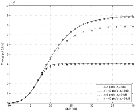
Figure 2: Theoretical and simulated throughput for the 2-way mechanism as a function of the SNR, for two different packet rates and capture thresholds, shown in the legend. Simulated points are identified by star-markers over the respective theoretical curves. Payload size is 1024 bytes, while the number of contending stations is $N=10$.

$$\small\frac{2}{\max(\log_{2}M,2)}\sum_{i=1}^{\max(\frac{M}{4},1)}\frac{1}{\pi}\int_{0}^{\frac{\pi}{2}}\frac{1}{1+\frac{\gamma\log_{2}M}{\sin^{2}\theta}\sin^{2}\left(\frac{(2i-1)\pi}{M}\right)}d\theta$$ (29)

whereby, $M$ is the number of bits per modulated symbols, $\gamma$ is the signal-to-noise ratio, and $\theta$ is the signal direction over the Rayleigh fading channel.

We note that the proposed DCF model is valid with any other PHY setup. Actually, all we need is simply the packet error rate probability $P_{e}(DATA,SNR)$ in (26) for the specific PHY and channel transmission conditions model. All the mathematical derivations proposed in this paper are specified with respect to $P_{e}(DATA,SNR)$, and so they are valid for any kind of transmission model at the PHY layer.

In what follows, we shall present theoretical and simulation results for the lowest supported data rate. We note that by repeating the process, similar curves can be generated for all other types of modulation formats. All we need is really the BER as a function of SNR for each modulation format and the corresponding raw data rate over the channel. If the terminals use rate adaptation, then under optimal operating condition, the achievable throughput for a given SNR is the maximum over the set of modulation formats supported. We have verified a close match between theoretical and simulated performances for other transmitting data rates as well. In the results presented below we assume the following values for the contention window: $CW_{min}=32$, $m=5$, and $CW_{max}=2^{m}\cdot CW_{min}=1024$.

Fig. 2 shows the behavior of the throughput for the 2-way mechanism as a function of the SNR, for two different capture thresholds, $z_{0}$, and packet rates, $\lambda$, as noted in the legend, and for $N=10$ transmitting stations. Simulated points are marked by star on the respective theoretical curves. Throughput increases as a function of the three parameters SNR, $\lambda$, and $z_{0}$ until saturation point.

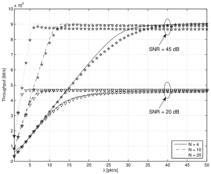
Figure 3: Theoretical and simulated throughput for the 2-way mechanism as a function of the packet rate $\lambda$, for three different number of contending stations and two different values of SNR as noted in the legend. Capture thresholds is $z_{0}=6$dB. Simulated points are identified by star-markers over the respective theoretical curves. Payload size is 1024 bytes.

Fig. 3 shows the behavior of the throughput as a function of $\lambda$, i.e., the packet rate, for three different values of the number of contending stations and for two values of SNR. The capture threshold is $z_{0}=6$dB. Beside noting the throughput improvement achievable for high SNR, notice that for a specified number of contending stations, the throughput manifests a linear behavior for low values of packet rates with a slope depending mainly on the number of stations $N$. However, for increasing values of $\lambda$, the saturation behavior occurs quite fast. Notice that, as exemplified in (25), $q\rightarrow 1$ as $\lambda\rightarrow\infty$. Actually, saturated traffic conditions are achieved quite fast for values of $\lambda$ on the order of ten packets per second with a number of contending stations greater than or equal to 10.

Fig. 4 shows the behavior of the throughput as a function of $\lambda$, for three different values of the number of contending stations and for two different SNRs. The capture threshold is $z_{0}=24$dB. We can draw conclusions similar to the ones derived for Fig. 3. Upon comparing the curves shown in Figs 3 and 4, it is easily seen that capture effects allow the system throughput to be almost the same independently from the number of stations in saturated conditions, i.e., for high values of $\lambda$.

Fig. 4 also shows the presence of a peak in the throughput as a function of $\lambda$, which characterizes the transition between the linear and saturated throughput. Such a peak tends to manifest itself for increasing values of $\lambda$ as the number of stations $N$ increases. A comparative analysis of the curves shown in Figs 3 and 4 reveals that the peak of the throughput tends to disappear because of the presence of capture effects during transmission.

Notice also that the throughput behavior exhibits saturation quite fast for low values of SNR independently from capture effects; this is essentially due to the fact that channel propagation errors tend to dominate over both collisions and capture when the SNR is low.

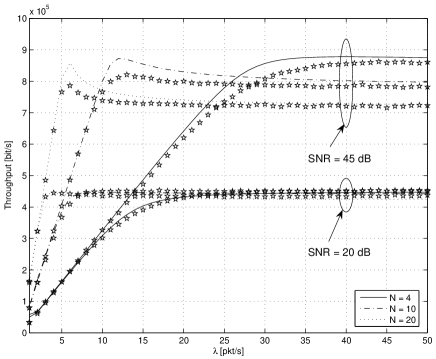
Figure 4: Theoretical and simulated throughput for the 2-way mechanism as a function of the packet rate $\lambda$, for three different number of contending stations and two different values of SNR as noted in the legend. Capture threshold is $z_{0}=24$dB. Simulated points are identified by star-markers over the respective theoretical curves. Payload size is 1024 bytes.

In order to assess throughput performances as a function of the payload size, Fig. 5 shows the behavior of the throughput as a function of $\lambda$, for a payload size equal to 128 bytes. The other simulation parameters are noted in the legend. Beside noting similar conclusions on the effects of both capture and number of contending stations over the throughput behavior as for the previous mentioned figures, notice also that a smaller payload size reduces proportionally the slope of the throughput before saturated conditions, and the maximum achievable throughput in saturated conditions. This issue will be dealt with in the next section.

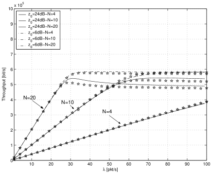
Figure 5: Theoretical and simulated throughput for the 2-way mechanism as a function of the packet rate $\lambda$, for three different number of contending stations and two different capture thresholds noted in the legend. Simulated points are identified by star-markers over the respective theoretical curves. Payload size is 128 bytes, while SNR=$45$dB.

IV-A Simulation results within ns-2

For the sake of validating the proposed model and our developed simulator against a widely adopted network simulator, while providing simulation results for a new set of parameters, we have performed new simulations using ns-2 (version 2.29) for throughput evaluations. Due to the lack of a complete PHY layer implementation, we made some modifications in the original ns-2 source code in order to account for a specific FER on the transmitted packets. In this respect, we adopted the suggestions proposed in [30] for simulating a 802.11b channel within ns-2. Briefly, channel errors on the transmitted packets are accounted for by using a uniformly distributed binary random variable $X_{e}$ with the following probabilities: $P(X_{e}=1)=P_{e}(SNR)$ (as specified in (26)), and $P(X_{e}=0)=1-P_{e}(SNR)$. For simplicity, we assume that data packets transmitted by different stations are affected by the same FER.

The employed propagation model is identified by the label Propagation/Shadowing within ns-2. We considered a path-loss exponent equal to 3.5 with a zero standard deviation in compliance with the theoretical capture scenario described above. Notice that the standard ns-2 simulator provides only Ad-Hoc support and related routing protocols; for this reason we applied a patch for implementing an Infrastructure BSS without any routing protocol between the various involved stations. This patch is identified by the acronym NOAH, standing for NO Ad-Hoc, and can be downloaded from http://icapeople.epfl.ch/widmer/uwb/ns-2/noah/.

In connection with the employed traffic model, we used an exponential distribution for simulating packet interarrival times.

Throughput evaluation is accomplished by averaging over $100$ sample scenarios, whereby any transmitting scenario considers a set of $N$ randomly distributed (with a uniform pdf) stations over a circular area of radius 10 m. Simulation results along with theoretical curves are shown in Figs 6-8. The employed parameters are noted in the respective legends of each figure. While the main conclusions related to the throughput behavior as a function of the number of contending stations, capture threshold, traffic load, and FER, are similar to the ones already derived above with our C++ simulator, here we notice a good agreement between theoretical and ns-2 simulation results for a wide range of packet arrival rates, $\lambda$.

Figs 6-7 also depict the theoretical saturated throughput derived by Bianchi in [13] in order to underline a good matching between our theoretical model, valid for any traffic load in the investigated range of $\lambda$ up to the saturation condition for $\lambda\rightarrow\infty$.

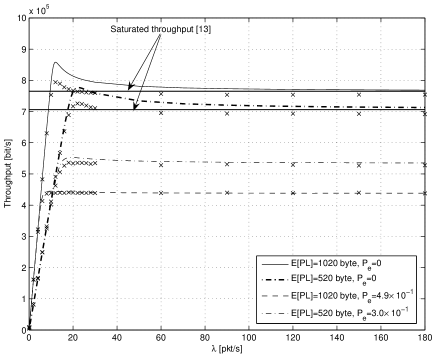
Figure 6: Theoretical and simulated (ns-2) throughput for the 2-way mechanism as a function of the packet rate $\lambda$, for two different payload sizes and packet error probabilities, shown in the legend, and without capture. Simulated points are identified by cross-markers over the respective theoretical curves. The number of contending stations is $N=10$.

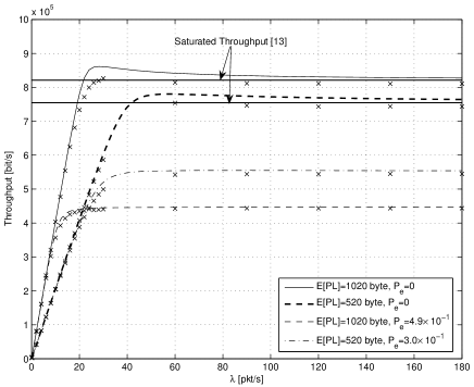
Figure 7: Theoretical and simulated (ns-2) throughput for the 2-way mechanism as a function of the packet rate $\lambda$, for two different payload sizes and packet error probabilities, shown in the legend, and without capture. Simulated points are identified by cross-markers over the respective theoretical curves. The number of contending stations is $N=5$.

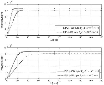
Figure 8: Both subplots show theoretical and simulated (ns-2) throughput for the 2-way mechanism as a function of the packet rate $\lambda$, for two different payload sizes and fixed packet error probability, as noted in the legend. Capture threshold $z_{0}=1$dB in both subplots. Simulated points are identified by cross-markers over the respective theoretical curves. Upper subplot refers to a number of contending stations equal to $N=10$, whereas the lower subplot corresponds to $N=5$.

V Modelling the linear behavior of the throughput in unsaturated conditions

The linear behavior of the throughput in unsaturated traffic conditions, along with its dependence on some key network parameters, can be better understood by analyzing the throughput in (18) as $\lambda\rightarrow 0$, i.e., in unloaded traffic conditions. From (10), it is easily seen that the probability $\tau\rightarrow 0$ when $\lambda\rightarrow 0$, since $q\rightarrow 0$. In particular, for very small values of $\lambda$, the following approximation from (10) holds:

$$\tau\simeq\frac{q}{1-P_{e}}$$

In addition, it is straightforward to verify that $P_{cap}\rightarrow 0$ (from (16)). As $\lambda$ approaches zero, the throughput can be approximated by:

$$S\simeq\frac{N(1-P_{e})E[PL]}{\sigma}\tau=\frac{N\cdot E[PL]}{\sigma}q=N\cdot E[PL]\cdot\lambda$$ (30)

since $q=1-e^{-\lambda E[S_{ts}]}$ can be approximated by $q\simeq E[S_{ts}]\lambda$ upon employing MacLaurin approximation of the exponential, and $E[S_{ts}]\rightarrow\sigma$ for $\lambda\rightarrow 0$ as it can be deduced from (23). The main conclusion that can be drawn from this equation is that as $\lambda\rightarrow 0$, the throughput tends to manifest a linear behavior relative to the packet rate $\lambda$ with a slope depending on both the number of contending stations and the average payload size $E[PL]$.

It is interesting to estimate the interval of validity $[0,\lambda_{c}]$ of the linear throughput model proposed in (30). To this end, let us rewrite (18) as follows:

$$\begin{array}[]{rcl}S&=&\frac{E[PL]}{\left[T_{s}-\frac{T_{c}}{1-P_{e}}+\frac{T_{e}P_{e}}{1-P_{e}}\right]+\frac{\sigma\frac{1-P_{t}}{P_{t}}+T_{c}}{P_{s}(1-P_{e})}}\\ \end{array}$$ (31)

Since $T_{s},T_{c},T_{e}$ and $P_{e}$ are independent of $\tau$, $S$ can be maximized by minimizing the function:

$$F(\tau)=\frac{\sigma\frac{1-P_{t}}{P_{t}}+T_{c}}{P_{s}(1-P_{e})}$$ (32)

or equivalently, by maximizing the function:

TABLE II: Values of $\lambda_{c}$ from (38) for the setup considered in Figs 4-5.

E[PL]=1024 byte	N=4	N=10	N=20
SNR=20dB	13.9187	5.5372	2.7638
SNR=45dB	26.7546	10.6444	5.3132
E[PL]=128 byte	N=4	N=10	N=20
SNR=45dB	135.0307	53.3990	26.6039

$$F_{1}(\tau)=\frac{1}{F(\tau)}=\frac{P_{s}(1-P_{e})}{\sigma\frac{1-P_{t}}{P_{t}}+T_{c}}$$ (33)

with respect to $\tau$. Upon substituting (19) and (20) in $F_{1}(\tau)$, it is possible to write:

$$F_{1}(\tau)=\frac{N\tau(1-P_{e})}{\sigma(1-\tau)+T_{c}(1-\tau)^{1-N}-T_{c}(1-\tau)}$$ (34)

Differentiating $F_{1}(\tau)$ with respect to $\tau$ and equating it to zero, it is possible to write:

$$\begin{array}[]{rcl}(1-\tau)^{N}(\sigma-T_{c})-T_{c}(N\tau-1)&=&0\\ \end{array}$$ (35)

Under the hypothesis $\tau\ll 1$, the following approximation holds:

$$(1-\tau)^{N}\approx 1-N\tau+\frac{N(N-1)}{2}\tau^{2}+o(\tau)$$

By substituting the previous approximation in (35), it is possible to obtain the value of $\tau$ maximizing $F_{1}(\tau)$:

$$\tau_{m}=\frac{\sigma-\sqrt{\sigma\left[N\sigma-2(N-1)(\sigma-T_{c})\right]/N}}{(N-1)(\sigma-T_{c})}$$ (36)

Substituting $\tau_{m}$ in (31), it is possible to obtain the maximum throughput $S_{m}$:

$$S_{m}=\frac{E[PL]}{\left[T_{s}-\frac{T_{c}}{1-P_{e}}+\frac{T_{e}P_{e}}{1-P_{e}}\right]+\frac{(\sigma-T_{c})(1-\tau_{m})^{N}+T_{c}}{N\tau_{m}(1-\tau_{m})^{N-1}(1-P_{e})}}$$ (37)

Equating $S_{m}$ to the linear model in (30), it is possible to obtain the value $\lambda_{c}$ for which the linear model reaches the beginning of the saturation zone, i.e., the maximum $\lambda$ above which the linear model loses validity:

$$\begin{array}[]{rl}\lambda_{c}=&\frac{1}{N\left[T_{s}-\frac{T_{c}}{1-P_{e}}+\frac{T_{e}P_{e}}{1-P_{e}}\right]+\frac{(\sigma-T_{c})(1-\tau_{m})^{N}+T_{c}}{\tau_{m}(1-\tau_{m})^{N-1}(1-P_{e})}}\\ \end{array}$$ (38)

The linear model (30) shows a close agreement with both theoretical and simulated throughput curves. Fig. 9 shows the straight lines (30) for three different values of the number of contending stations $N$, compared with the theoretical curves already depicted in Fig. 4. The figure also shows the values of $S_{m}$ as derived from (37) along with the three values of $\lambda_{c}$ deduced from (38). Notice that $\lambda_{c}$, besides being the limit of validity of the linear model, can also be interpreted as the value of packet rate above which the throughput enters saturation conditions.

In order to further verify the values of $\lambda_{c}$ deduced from (38), Table II shows the values of $\lambda_{c}$ related to both simulation and theoretical results depicted in Figs 4-5. In particular, values shown in the upper part of the table, i.e., the ones labelled E[PL]=1024, are related to the curves in Fig. 4, whereas the other values are related to the results in Fig. 5. Notice the good agreement between theoretical and simulated results even in the presence of capture. The key observation here can be deduced by a comparative analysis of the results shown in Figs. 3-4: capture tends to simply shape the peak on which the throughput reaches its maximum, leaving the abscissa of the maximum, that is $\lambda_{c}$, in the same position.

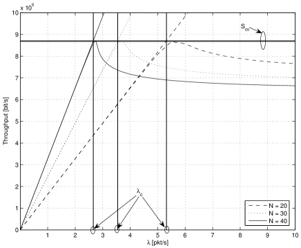
Figure 9: Throughput for the 2-way mechanism as a function of the packet rate $\lambda$, for three different number of contending stations. Capture threshold and SNR are set to very high values since in pre-saturation regime. Payload size is 1024 bytes. Straight lines refer to the linear model of the throughput derived in (30).

VI Conclusions

In this paper, we have provided an extension of the Markov model characterizing the DCF behavior at the MAC layer of the IEEE802.11 series of standards by accounting for channel induced errors and capture effects typical of fading environments under unsaturated traffic conditions. The modelling allows taking into consideration the impact of channel contention in throughput analysis which is often not considered or it is considered in a static mode by using a mean contention period. Subsequently, based on justifiable assumptions, the stationary probability of the Markov chain is calculated to obtain the behavior of the throughput in both unsaturated and saturated conditions. The closed form expressions allow derivation of the throughput as a function of a multitude of system level parameters including packet and header sizes for a variety of applications. Simulation results confirm the validity of the proposed theoretical models.

References

- [1] IEEE Standard for Wireless LAN Medium Access Control (MAC) and Physical Layer (PHY) Specifications, November 1997, P802.11
- [2] Wei Zhuang, Yung-Sze Gan, Kok-Jeng Loh, and Kee-Chaing Chua, ”Policy-based QoS-management architecture in an integrated UMTS and WLAN environment”, IEEE Communications Magazine, Vol.41, No.11, pp.118-125, Nov. 2003.
- [3] W. Liu, W. Lou, X. Chen, and Y. Fang, ”A QoS-enabled MAC architecture for prioritized service in IEEE 802.11 WLANs”, Proc. IEEE GLOBECOM’03, Vol.7, pp.3802-3807, Dec. 2003.
- [4] G. Fodor, A. Eriksson, and A. Tuoriniemi, ”Providing quality of service in always best connected networks”, IEEE Communications Magazine, Vol.41, No.7, pp.154-163, July 2003.
- [5] J. Zhao, Z. Guo, Q. Zhang, and W. Zhu, ”Performance study of MAC for service differentiation in IEEE 802.11”, In Proc. of IEEE GLOBECOM’02, Vol.1, pp.778-782, Nov. 2002.
- [6] W. Pattara-Atikom, P. Krishnamurthy, and S. Banerjee, ”Distributed mechanisms for quality of service in wireless LANs”, IEEE Personal Communications, Vol.10, No.3, pp.26-34, June 2003.
- [7] Ye Ge and J. Hou, ”An analytical model for service differentiation in IEEE 802.11”, Proc. ICC ’03, Vol.2, pp.1157-1162, May 2003.
- [8] H. L. Truong and G. Vannuccini, ”Performance evaluation of the QoS enhanced IEEE 802.11e MAC layer”, In Proc. of IEEE VTC 2003-Spring, Vol.2, pp.940-944, April 2003.
- [9] Q. Li and M. VanderSchaar, ”Providing adaptive QoS to layered video over wireless local area networks through real-time retry limit adaptation”, IEEE Trans. on Multimedia, Vol.6, No.2, pp.278-290, April 2004.
- [10] Q. Zhang, C. Guo, Z. Guo, and W. Zhu, ”Efficient mobility management for vertical handoff between WWAN and WLAN”, IEEE Communications Magazine, Vol.41, No.11, pp.102-108, Nov. 2003.
- [11] H. Honkasalo, K. Pehkonen, M. T. Niemi, and A.T. Leino, ”WCDMA and WLAN for 3G and beyond”, IEEE Personal Communications, Vol.9, No.2, pp.14-18, April 2002.
- [12] S. Park, K. Kim, D.C. Kim, S. Choi, and S. Hong, ”Collaborative QoS architecture between DiffServ and 802.11e wireless LAN”, In Proc. of IEEE VTC 2003-Spring, Vol.2, pp.945-949, April 2003.
- [13] G. Bianchi, ”Performance analysis of the IEEE 802.11 distributed coordination function”, IEEE JSAC, Vol.18, No.3, March 2000.
- [14] L. Yong Shyang, A. Dadej, and A.Jayasuriya, ”Performance analysis of IEEE 802.11 DCF under limited load”, In Proc. of Asia-Pacific Conference on Communications, Vol.1, pp.759 - 763, 03-05 Oct. 2005.
- [15] M. Ergen and P. Varaiya, ”Throughput analysis and admission control in IEEE 802.11a”, Springer Mobile Networks and Applications, vol. 10, no. 5., pp. 705-706, October 2005.
- [16] J.W. Robinson and T.S. Randhawa ”Saturation throughput analysis of IEEE 802.11e enhanced distributed coordination function”, IEEE JSAC, Vol.22, No.5, June 2004.
- [17] Z. Kong, D.H.K. Tsang, B.Bensaou, and D.Gao, ”Performance analysis of IEEE 802.11e contention-based channel access”, IEEE JSAC, Vol.22, No.10, Dec. 2004.
- [18] D. Qiao, S. Choi, and K.G. Shin ”Goodput analysis and link adaptation for IEEE 802.11a wireless LANs”, IEEE Trans. On Mobile Computing, Vol.1, No.4, Oct.-Dec. 2002.
- [19] P. Chatzimisios, A.C. Boucouvalas, and V. Vitsas, ”Influence of channel BER on IEEE 802.11 DCF”, IEE Electronics Letters, Vol.39, No.23, pp.1687-1689, Nov. 2003.
- [20] Q. Ni, T. Li, T. Turletti, and Y. Xiao, ”Saturation throughput analysis of error-prone 802.11 wireless networks”, Wiley Journal of Wireless Communications and Mobile Computing, Vol. 5, No. 8, pp. 945-956, Dec. 2005.
- [21] K. Duffy, D. Malone, and D.J. Leith, ”Modeling the 802.11 distributed coordination function in non-saturated conditions”, IEEE Communications Letters, Vol.9, No.8, pp.715-717, Aug. 2005.
- [22] Jae Hyun Kim and Jong Kyu Lee ”Capture effects of wireless CSMA/CA protocols in Rayleigh and shadow fading channels”, IEEE Trans. on Veh. Tech., Vol.48, No.4, pp.1277-1286, July 1999.
- [23] M. Zorzi and R.R. Rao, ”Capture and retransmission control in mobile radio”, IEEE JSAC, Vol.12, No.8, pp.1289 - 1298, Oct. 1994.
- [24] Z. Hadzi-Velkov and B. Spasenovski, ”Capture effect in IEEE 802.11 basic service area under influence of Rayleigh fading and near/far effect”, In Proc. of 13th IEEE International Symposium on Personal, Indoor and Mobile Radio Communications, Vol.1, pp.172 - 176, Sept. 2002.
- [25] M. B. Pursley, ”Performance evaluation for phase-coded spread spectrum multiple-access communication Part I: System analysis”, IEEE Trans. Commun., vol. COM-25, pp. 795 799, Aug. 1977.
- [26] T. S. Ho and K. C. Chen, ”Performance evaluation and enhancement of the CSMA/CA MAC protocol for 802.11 wireless LAN s”, In Proc. of IEEE PIMRC, Taipei, Taiwan, Oct. 1996, pp. 392 396.
- [27] D. Malone, K. Duffy, and D.J. Leith, ”Modeling the 802.11 distributed coordination function in non-saturated heterogeneous conditions”, IEEE-ACM Trans. on Networking, vol. 15, No. 1, pp. 159 172, Feb. 2007.
- [28] M.K. Simon and M. Alouini, Digital Communication over Fading Channels: A Unified Approach to Performance Analysis, Wiley-Interscience, 1st edition, 2000.
- [29] T. Rappaport, Wireless Communications, Prentice Hall, 1999.
-
[30]
Wu Xiuchao, ”Simulate 802.11b Channel within NS-2”, available
online at
http://www.comp.nus.edu.sg/~wuxiucha/research/reactive/report/80211ChannelinNS2_new.pdf