Saturation Throughput Analysis of IEEE 802.11 in Presence of Non Ideal Transmission Channel and Capture Effects

Abstract

In this paper, we provide a saturation throughput analysis of the IEEE 802.11 protocol at the data link layer by including the impact of both transmission channel and capture effects in Rayleigh fading environment. Impacts of both non-ideal channel and capture effects, specially in an environment of high interference, become important in terms of the actual observed throughput. As far as the 4-way handshaking mechanism is concerned, we extend the multi-dimensional Markovian state transition model characterizing the behavior at the MAC layer by including transmission states that account for packet transmission failures due to errors caused by propagation through the channel. This way, any channel model characterizing the physical transmission medium can be accommodated, including AWGN and fading channels. We also extend the Markov model in order to consider the behavior of the contention window when employing the basic 2-way handshaking mechanism.

Under the usual assumptions regarding the traffic generated per node and independence of packet collisions, we solve for the stationary probabilities of the Markov chain and develop expressions for the saturation throughput as a function of the number of terminals, packet sizes, raw channel error rates, capture probability, and other key system parameters. The theoretical derivations are then compared to simulation results confirming the effectiveness of the proposed models.

I Introduction

Wireless Local Area Networks (WLANs) combine data connectivity with user mobility. The Institute of Electrical and Electronic Engineering (IEEE) 802.11 series of standards define both an infrastructure mode, with at least one central Access Point (AP) connected to a wired network, and an ad-hoc or peer-to-peer mode, in which a set of wireless stations communicate directly with another one without needing a central access point or wired network connection.

WLANs have experienced an exponential growth in the recent past [1-20]. The fundamental impetus has been to replicate the enormous success of wired LANs with obvious advantages a wireless paradigm would bring. The first series of standards by IEEE was ratified in 1997 but had relatively low data rates (1 or 2 Mbps). Two high rate versions, namely, the IEEE802.11a and IEEE802.11b were later ratified in 1999 and they have found widespread acceptance and use. The enormous success of these standards has prompted multiple working groups to extend some aspects of the basic protocol.

While in the ensuing presentation we shall focus on the basic IEEE802.11b protocol, the analysis is easily extensible to other versions of the basic protocol employing the same Medium Access Control (MAC) mechanisms.

The MAC is central to embedding Quality of Service (QoS) features and has two sub-layers [1]. The Distributed Coordination Function (DCF) and Point Coordination Function (PCF). PCF is generally a complex access method that can be implemented in an infrastructure network. DCF is similar to Carrier Sense Multiple Access with Collision Avoidance (CSMA/CA) method and is further explained in the following.

With this background, let us provide a quick survey of the recent literature related to the problem addressed in this paper. This survey is by no means exhaustive and is meant to simply provide a sampling of the literature in this fertile area.

The most relevant work to what is presented here is [2], where the author provided an analysis of the saturation throughput of the basic 802.11 protocol assuming a two dimensional Markov model at the MAC layer, making several fundamental assumptions: 1) the mobile stations always have something to transmit (i.e., the saturation condition), 2) there are no hidden terminals and there is no capture effect (i.e., a terminal which perceives a higher signal-to-noise ratio (SNR) relative to other terminals captures the channel [3, 4, 5] and limits access to other terminals), 3) at each transmission attempt and regardless of the number of retransmissions suffered, each packet collides with constant and independent probability, and 4) the transmission channel is ideal and the only cause of packet errors are collisions. Clearly, the second and fourth assumption is not valid in any real setting, specially when there is mobility and when the transmission channel suffers from fading effects.

In [6], the authors extend the work of Bianchi to multiple queues with different contention characteristics in the 802.11e variant of the standard with provisions of QoS. In [7], the authors present an analytical model, in which most new features of the Enhanced Distributed Channel Access (EDCA) in 802.11e such as virtual collision, different arbitration interframe space (AIFS), and different contention windows are taken into account. Based on the model, the throughput performance of differentiated service traffic is analyzed and a recursive method capable of calculating the mean access delay is presented. Both articles referenced assume the transmission channel to be ideal.

In [8], the authors look at the impact of channel induced errors and the received SNR on the achievable throughput in a system with rate adaptation whereby the transmission rate of the terminal is adapted based on either direct or indirect measurements of the link quality. In [9], the authors deal with the extension of Bianchi’s Markov model in order to account for channel errors.

In this article we extend the previous work on the subject as exemplified by the articles referenced above by looking at all the three issues outlined before together. Our assumptions are essentially similar to those of Bianchi [2] with the exception that we do assume the presence of both channel induced errors and capture effects due to the transmission over Rayleigh fading channels. Simulation results confirm the effectiveness of the proposed models. As a reference standard, we use network parameters belonging to the IEEE802.11b protocol, even though the proposed mathematical models hold for any flavor of the IEEE802.11 family.

The rest of the article is organized as follows. Section II reviews the functionalities of the contention window procedure at MAC layer. Section III extends the Markov model initially proposed by Bianchi, presenting modifications that account for transmission errors and capture effects over Rayleigh fading channels employing the 4-way handshaking technique. This section also provides an expression for the saturation throughput of the link. In section IV we briefly extend the analysis of the two dimensional Markov chain for the basic 2-way handshaking mechanism. In section V we present simulation results where typical MAC layer parameters for IEEE802.11b are used to obtain throughput values as a function of various system level parameters, capture probability, and SNR. Section VI is devoted to conclusions.

II Development of the Markov Model

In this section, we present the rationales at the basis of the proposed bi-dimensional Markov model useful for evaluating the throughput of the DCF under the assumptions of finite number of operating terminals, channel error conditions, capture effects in Rayleigh fading transmission scenario, and packet transmission based on the four-way handshaking access mechanism. For conciseness, we will limit our presentation to the ideas needed for developing the proposed model. We invite the interested readers to refer to [1, 2] for many details on the operating functionalities of the DCF.

II-A Markovian Model Characterizing the MAC Layer: Perfect Transmission Channel

In [2], a discrete-time bi-dimensional Markov process $(s(t),b(t))$ is presented for the computation of the throughput of a WLAN using the IEEE 802.11 DCF under ideal channel conditions.

It is based on two key assertions:

1. the probability $\tau$ that a station will attempt transmission in a generic time slot is constant across all time slots;

2. the probability $P_{col}$ that any transmission experiences a collision is constant and independent of the number of collisions already suffered.

The random process $b(t)$ is used to represent the backoff counter of each station. Backoff counter is decremented at the start of every idle backoff slot and when it reaches zero, the station transmits and a new value for $b(t)$ is set. The value of $b(t)$ after each transmission depends on the size of the contention window from which it is drawn. A second process $s(t)$ is defined, representing the size of the contention window $(W_{i}=2^{i}W,~{}i=s(t))$ from which $b(t)$ is drawn.

We recall that a backoff time counter is initialized depending on the number of failed transmissions for the transmitted packet. It is chosen from the range $[0,W_{i}-1]$ following a uniform Probability Mass Function (PMF), where $W_{i}$ is the contention window size at the backoff stage $i$. At the first transmission attempt (i.e., for $i=0$), the contention window size is set equal to a minimum value $W_{0}=W$, and the process $s(t)$ takes on the value $s(t)=i=0$.

The backoff stage $i$ is incremented in unitary steps after each unsuccessful transmission up to the maximum value $m$, while the contention window is doubled at each stage up to the maximum value $CW_{max}=2^{m}W$.

The backoff time counter is decremented as long as the channel is sensed idle and stopped when a transmission is detected. The station transmits when the backoff time counter reaches zero.

III Markovian Model Characterizing the MAC Layer under Real Transmission Channel and Capture Effects Using the 4-Way Handshaking Mechanism

The main aim of this section is to propose an effective modification of the bi-dimensional Markov process proposed in [2] in order to account for channel error conditions and capture effects over Rayleigh fading channel under the hypothesis of employing the four-way handshaking access mechanism. It is useful to briefly recall the four-way handshaking mechanism for highlighting the hypotheses at the basis of the proposed Markov model.

A station that wants to transmit a packet, waits until the channel is sensed idle for a Distributed InterFrame Space (DIFS), follows the backoff rules and then preliminarily transmits a short Request To Send (RTS) frame. The receiving station, after having received an RTS frame, responds with a Clear To Send (CTS) frame, after a Short InterFrame Space (SIFS). The transmitting station is allowed to transmit its packet only after having correctly received the CTS frame. Both RTS and CTS frames carry the information about the length of the packet to be transmitted. This information is available to any listening station, so that they can update their Network Allocation Vector (NAV) with the information about the period of time in which the channel will be busy. Therefore, every station, hidden from either the transmitting or the receiving station, by detecting just one frame among the RTS and CTS frames, can delay transmissions by an appropriate amount, thus avoiding collisions.

On the basis of this assumption, collisions can only occur with probability $P_{col}$ on RTS packets, while transmission errors, due to the channel, can occur with probability $P_{e}$ only on the data frames. Therefore, if a station is free to send a data frame (that means that the transmitting station received the CTS frame), it can start the data frame transmission. This frame is protected from collision, but not from transmission errors. In this work, we assume that collision and transmission error events are statistically independents.

Furthermore, in mobile radio environment, it may happen that the channel is captured by a station whose power level is stronger than the other stations transmitting at the same time. This may be due to relative distances and/or channel conditions for each user and may happen whether or not the terminals exercise power control. As a matter of fact, capture effect reduces the collision probability on the channel, since the stations whose power level at the receiver is very low due to path attenuation, shadowing and fading, are considered as interferers from the AP, thus raising the noise floor.

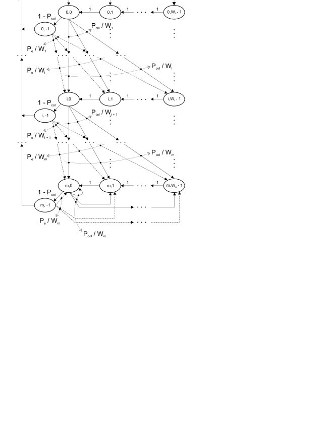
Figure 1: Markov chain for the contention model based on the 4-way handshaking technique, considering the effects of capture and channel induced errors.

To account for these phenomena, our Markov chain model depicted in Fig. 1 includes a Transmit (TX) state, identified by $(i,-1),~{}\forall i=0,\ldots,m$, which is not considered in the original work of Bianchi in [2]. To reach the transmit state, there should be no collision or a collision in which the desired station captures the channel (hence, in effect no collision is detected even though there is one).

To simplify the analysis, we make the assumption that the impact of the channel induced errors on the RTS, CTS and Acknowledgment (ACK) packets are negligible because of their short length. This is justified on the basis of the assumption that the bit errors inflicting the transmitted data are independent of each other. Hence, the packet or frame error rate, identified respectively with the acronyms PER or FER, is a function of the packet length, with shorter packets having exponentially smaller probability of error compared to longer packets.

Notice that FER in general also depends on the forward error correcting code employed at the physical layer [21, 22]. However, for convolutional coding, as optionally foreseen in the IEEE 802.11b standard [1], bit error rate (BER) is independent from the code block size, and, as a consequence, FER assumes increasing values for larger and larger data packet sizes. It is known that the BER for convolutional codes depends on the distance spectrum of the code [23]-[25] which is independent of the block size.

We note that with sufficient interleaving we can always ensure that the errors inflicting individual bits in a data packet are independent of each other. Since the length of the ACK, CTS and RTS frames are typically less than 20 bytes, while the information baring packets are typically several hundreds of bytes long, the assumption is clearly justified. Including the possibility that the ACK, RTS and CTS frames can themselves be erroneous unduly complicates an already complex Markov chain with no clear benefits.

Let us discuss the Markov model shown in Fig. 1. Similar to the model in [2], $(m+1)$ different backoff stages are considered (this includes the zero-th stage). The maximum contention windows (CW) sizes is then $CWmax=2^{m}W$, and the relation $W_{i}=2^{i}W$ is used to define the $i^{th}$ contention window size. An RTS can be transmitted only in the $(i,0)$ states, $\forall i=0,\ldots,m$, while data can only be transmitted in the $(i,-1)$ states, $\forall i=0,\ldots,m$ upon a successful reception of the CTS. If collision occurs, the backoff stage is incremented, so that the new state can be $(i+1,k)$ with probability $P_{col}/W_{i+1}$, since a uniform distribution between the states in the same backoff stage is considered. We consider capture as a subset of the event of a collision. In other words, the capture event can happen in the presence of collision, by allowing the transmitting station with the higher received power level at the access point to capture the channel. In this case, there is no collision and the Markov model transits into one of the transmitting states $(i,-1)$ depending on the current contention stage. If no collision occurs, a data frame can be transmitted, and the transmitting station enters state $(i,-1)$, based on the backoff stage it belongs to. From state $(i,-1)$, if the transmission is successful, the transmitting station re-enters the initial backoff stage, identified by $i=0$. Otherwise, if errors occur during transmission, the ACK packet is not sent, an ACK-timeout occurs, and the backoff stage is changed to $(i+1,k)$ with probability $P_{e}/W_{i+1}$, where $P_{e}$ is the packet error probability for the employed physical layer.

The Markov Process of Fig. 1 is governed by the following transition probabilities:

$$\small\begin{array}[]{lll}P_{i,k|i,k+1}&=1,&~{}k\in[0,W_{i}-2],~{}i\in[0,m]\\ P_{i,-1|i,0}&=1-P_{col},&~{}k=0,~{}i\in[0,m]\\ P_{0,k|i,-1}&=(1-P_{e})/W_{0},&~{}k\in[0,W_{0}-1],~{}i\in[0,m]\\ P_{i,k|i-1,0}&=P_{col}/W_{i},&~{}k\in[0,W_{i}-1],~{}i\in[1,m]\\ P_{i,k|i-1,-1}&=P_{e}/W_{i},&~{}k\in[0,W_{i}-1],~{}i\in[1,m]\\ P_{m,k|m,0}&=P_{col}/W_{m},&~{}k\in[0,W_{m}-1]\\ P_{m,k|m,-1}&=P_{e}/W_{m},&~{}k\in[0,W_{m}-1]\end{array}$$ (1)

The first equation in (1) states that, at the beginning of each slot time, the backoff time is decremented. The second equation accounts for the fact that after a successful RTS transmission and CTS reception, the data transmission state is $(s(t)=i,b(t)=-1)$ with probability $1-P_{col}$. The third equation accounts for the fact that after a successful transmission, a new packet transmission starts with backoff stage 0. The other equations deal with unsuccessful transmissions. Capture effects are accounted for in the definition of the collision probability. The fourth and sixth equations deal with RTS frame collisions. In this case, a new backoff stage is scheduled. Finally, the fifth and seventh equations model failed transmissions due to channel induced errors. In this situation, a new backoff stage is scheduled as well.

III-A Markovian Process Analysis and Throughput Computation

Next line of pursuit consists in finding a solution of the stationary distribution:

$$b_{i,k}=\lim_{t\rightarrow\infty}P[s(t)=i,b(t)=k],~{}\forall k\in[-1,W_{i}-1],~{}\forall i\in[0,m]$$

that is the probability of a station occupying a given state at any discrete time.

For the sake of simplifying the evaluation of the normalization condition of the bidimensional Markov chain, let us express all the probabilities $b_{i,k}$ as a function of $b_{0,0}$. To this end, note the following relations:

$$\begin{array}[]{ll}b_{i,-1}=b_{i,0}\left(1-P_{col}\right),~{}\forall i\in[0,m]&\\ b_{i,0}=b_{i-1,-1}P_{e}+b_{i-1,0}P_{col},~{}\forall i\in[1,m)&\\ \end{array}$$ (2)

while for $i=m$ we have:

$$\begin{array}[]{ll}b_{m,0}=b_{m-1,-1}P_{e}+b_{m-1,0}P_{col}+&\\ +b_{m,-1}P_{e}+b_{m,0}P_{col}&\end{array}$$

from which it is possible to obtain:

$$\begin{array}[]{ll}b_{m,0}\left(1-P_{col}\right)=b_{m-1,-1}P_{e}+b_{m,-1}P_{e}+&\\ +b_{m-1,0}P_{col}&\end{array}$$

These relations will be used later for solving the normalization condition applied to the bi-dimensional Markov model shown in Fig. 1.

Upon defining an equivalent probability of failed transmission, $P_{eq}$, that takes into account the need for a new contention due to either RTS collision ($P_{col}$) or channel errors affecting the data frame ($P_{e}$), i.e.,

$$P_{eq}=P_{col}+P_{e}-P_{e}\cdot P_{col}$$ (3)

after some simple algebra involving the previous relations, it is possible to obtain the following relations:

$$\begin{array}[]{ll}b_{i,0}=P_{eq}b_{i-1,0},&~{}\forall i\in[1,m)\\ b_{m,0}=P_{eq}b_{m-1,0}+P_{eq}b_{m,0},&~{}i=m\end{array}$$ (4)

Proceeding backward, the following results follow by inspection:

$$\begin{array}[]{ll}b_{i,0}=P_{eq}^{i}b_{0,0},&~{}\forall i\in[1,m)\\ b_{m,0}=\frac{P_{eq}^{m}}{1-P_{eq}}b_{0,0},&~{}i=m\end{array}$$ (5)

The other stationary probabilities for any $k\in[1,W_{i}-1]$ follow by resorting to the state transition diagram:

$$b_{i,k}=\frac{W_{i}-k}{W_{i}}\left\{\begin{array}[]{ll}(1-P_{e})\sum_{j=0}^{m}b_{j,-1},&~{}i=0\\ P_{col}b_{i-1,0}+P_{e}b_{i-1,-1},&~{}i\in[1,m)\\ P_{col}(b_{m-1,0}+b_{m,0})+\\ +P_{e}(b_{m-1,-1}+b_{m,-1}),&~{}i=m\end{array}\right.$$ (6)

Employing the normalization condition, after some mathematical manipulations, it is possible to obtain:

$$\small\begin{array}[]{l}1=\sum_{i=0}^{m}\sum_{k=-1}^{w_{i}-1}b_{i,k}=b_{0,0}\frac{2(1-P_{eq})W(1-(2P_{eq})^{m-1})P_{eq}+P_{x}(1-P_{col})\left((1-P_{e})(W+1)+2\right)+P_{x}(1-P_{eq}^{m-1})P_{eq}+(2^{m}W+1)P_{x}P_{eq}^{m}}{2P_{x}(1-P_{eq})}\end{array}$$ (7)

whereby, $P_{x}=1-2P_{eq}$. Normalization condition yields the following equation for computation of $b_{0,0}$:

$$\small\begin{array}[]{ll}b_{0,0}=\frac{2P_{x}(1-P_{eq})}{2(1-P_{eq})W(1-(2P_{eq})^{m-1})P_{eq}+P_{x}(1-P_{col})\left((1-P_{e})(W+1)+2\right)+P_{x}(1-P_{eq}^{m-1})P_{eq}+(2^{m}W+1)P_{x}P_{eq}^{m}}\end{array}$$ (8)

This result is then used to compute $\tau$, the probability that a station starts a transmission in a randomly chosen slot time. In fact, taking into account that an RTS transmission occurs when the backoff counter reaches zero, we have:

$$\begin{array}[]{ll}\tau=\sum_{i=0}^{m}b_{i,0}=\frac{b_{0,0}}{1-P_{eq}}=\frac{2P_{x}}{2(1-P_{eq})W(1-(2P_{eq})^{m-1})P_{eq}+P_{x}(1-P_{col})\left((1-P_{e})(W+1)+2\right)+P_{x}(1-P_{eq}^{m-1})P_{eq}+(2^{m}W+1)P_{x}P_{eq}^{m}}\end{array}$$ (9)

The collision probability, needed to compute $\tau$, can be found considering that using a 4-way hand-shaking an RTS frame from a transmitting station encounters a collision if in a time slot, at least one of the remaining $(N-1)$ stations transmit simultaneously an RTS frame, and there is no capture. In our model, we assume that capture is a subset of the collision events. This is indeed justified by the fact that there is no capture without collision, and that capture occurs only because of collisions between a certain number of transmitting stations attempting to transmit simultaneously on the channel.

$$P_{col}=1-(1-\tau)^{N-1}-P_{cap}$$ (10)

As far as capture effects are concerned, we resort to the mathematical formulation proposed in [4, 5]. In particular, under the hypothesis of power-controlled stations in infrastructure mode, the capture probability conditioned on $i$ interfering frames can be defined as follows:

$$P_{cp}\left(\gamma>z_{o}g(S_{f})|i\right)=\frac{1}{{\left[1+z_{0}g(S_{f})\right]}^{i}}$$ (11)

whereby $\gamma$, defined as $P_{u}/\sum_{k=1}^{i}P_{k}$, is the ratio of the power $P_{u}$ of the useful signal and the sum of the powers of the $i$ interfering channel contenders transmitting simultaneously $i$ frames, $g(S_{f})$ is the inverse of the processing gain of the correlation receiver, and $z_{0}$ is the capture ratio, i.e., the value of the signal-to-interference power ratio identifying the capture threshold at the receiver. Notice that (11) signifies the fact that capture probability corresponds to the probability that the power ratio $\gamma$ is above the capture threshold $z_{0}g(S_{f})$ which considers the inverse of the processing gain $g(S_{f})$. For Direct Sequence Spread Spectrum (DSSS) using a 11-chip spreading factor ($S_{f}=11$), we have $g(S_{f})=\frac{2}{3S_{f}}$.

Upon defining the probability of generating exactly $i+1$ interfering frames over $N$ contending stations in a generic slot time:

$${N\choose i+1}\tau^{i+1}(1-\tau)^{N-i-1}$$

the frame capture probability $P_{cap}$ can be obtained as follows:

$$P_{cap}=\sum_{i=1}^{N-1}{N\choose i+1}\tau^{i+1}(1-\tau)^{N-i-1}P_{cp}\left(\gamma>z_{o}g(S_{f})|i\right)$$ (12)

Putting together equations (3), (9), (10) and (12), the following nonlinear system can be defined and solved numerically, obtaining the values of $\tau$ (defined in (9)), $P_{col}$, $P_{eq}$, and $P_{cap}$:

$$\left\{\begin{array}[]{ll}\tau&\\ P_{col}&=1-(1-\tau)^{N-1}-P_{cap}\\ P_{eq}&=P_{col}+P_{e}-P_{e}\cdot P_{col}\\ P_{cap}&=\sum_{i=1}^{N-1}{N\choose i+1}\tau^{i+1}(1-\tau)^{N-i-1}\frac{1}{{(1+z_{0}g(S_{f}))}^{i}}\end{array}\right.$$ (13)

The final step in the analysis is the computation of the normalized system throughput, defined as the fraction of time the channel is used to successfully transmit payload bits:

$$\small S=\frac{P_{t}\cdot P_{s}\cdot(1-P_{e})E[PL]}{(1-P_{t})\sigma+P_{t}(1-P_{s})T_{c}+P_{t}P_{s}(1-P_{e})T_{s}+P_{t}P_{s}P_{e}T_{e}}$$ (14)

where

• $P_{t}$ is the probability that there is at least one transmission in the considered slot time, with $N$ stations contending for the channel, each transmitting with probability $\tau$:

  $$P_{t}=1-(1-\tau)^{N}$$ (15)

• $P_{s}$ is the conditional probability that an RTS transmission occurring on the channel is successful. This event corresponds to the case in which exactly one station transmits in a given slot time, or two or more stations transmit simultaneously and capture by the desired station occurs. These conditions yields the following probability:

  $$P_{s}=\frac{N\tau(1-\tau)^{N-1}+P_{cap}}{P_{t}}$$ (16)

• $T_{c}$, $T_{e}$ and $T_{s}$ are the average time a channel is sensed busy due to an RTS collision, error affected data frame transmission time and successful data frame transmission times, respectively. Knowing the time durations for RTS, CTS, ACK frames, CTS and ACK timeout, DIFS, SIFS, $\sigma$, data packet length ($PL$) and PHY and MAC headers duration ($H$), and propagation delay $\tau_{p}$, $T_{c}$, $T_{s}$, and $T_{e}$ can be computed as follows [7]:

  $$\begin{array}[]{ll}T_{c}&=RTS+CTS_{timeout}\\ T_{e}&=RTS+SIFS+\tau_{p}+CTS+SIFS+\tau_{p}+\\ &+H+PL+ACK_{timeout}\\ T_{s}&=RTS+SIFS+\tau_{p}+CTS+SIFS+\tau_{p}+\\ &+H+PL+SIFS+\tau_{p}+ACK+DIFS+\tau_{p}\\ \end{array}$$ (17)

• $E[PL]$ is the average packet payload length.

• $\sigma$ is the duration of an empty slot time.

The setup described above is used in Section V for DCF simulation at the MAC layer.

IV Analysis of the Markov chain for the basic 2-way handshaking mechanism in presence of channel errors and capture effects

This section briefly provides the extension of the Markov model for the contention model to the case of using the basic two-way handshaking mechanism.

Let us review the basic functionalities of the two-way handshaking technique. No RTS/CTS exchange of packets is used. After the successful reception of a data frame, the receiver sends an ACK frame to the transmitter. Only upon a correct ACK frame reception, the transmitter assumes successful delivery of the corresponding data frame. If an ACK frame is received in error or if no ACK frame is received, due possibly to an erroneous reception of the preceding data frame, the transmitter will contend again for the medium.

Based on these assumptions, using the two-way handshaking mechanism there is no evident distinction between the transmission of information and protocol data. In this respect, the Markov chain model for the backoff window size can be represented as in Bianchi’s model [2] upon exchanging $p$, the collision probability, with the probability $P_{eq}$ defined in (3). Notice that transmission fails when collision occurs between packets, or when data transmission is affected by channel errors with probability $P_{e}$. As far as collision is concerned, capture effects reduce the probability of collision by an amount equal to $P_{cap}$, i.e., the probability of capture. So, in this respect, rationales are the same as for the 4-way handshaking mechanism discussed above.

Upon defining $P_{eq}$ as in (3), the stationary distribution of the Bianchi’s Markov chain can be evaluated by following the same mathematical derivations dealt with in Bianchi’s model [2] whereby $P_{eq}$ is used in place of $p$. Finally, the throughput is evaluated through (14) upon solving the non-linear system of equations in (13).

IV-A Markovian Process Analysis and Throughput Computation

The objective is finding a solution of the stationary distribution:

$$b_{i,k}=\lim_{t\rightarrow\infty}P[s(t)=i,b(t)=k],~{}\forall i\in[0,m],~{}\forall k\in[0,W_{i}-1],$$

that is the probability of a station occupying a given state at any discrete slot time.

First of all, note that for any $i\in[1,m)$ the following relation holds:

$$\begin{array}[]{ll}b_{i,0}=b_{i-1,0}P_{eq},&~{}\forall i\in[1,m)\\ b_{m,0}=b_{m-1,0}P_{eq}+b_{m,0}P_{eq},&~{}i=m\end{array}$$ (18)

Proceeding backward, the following results follow by inspection:

$$\begin{array}[]{ll}b_{i,0}=P_{eq}^{i}\cdot b_{0,0},&~{}\forall i\in[1,m)\\ b_{m,0}=\frac{P_{eq}^{m}}{1-P_{eq}}\cdot b_{0,0},&~{}i=m\end{array}$$ (19)

The stationary probabilities for any $k\in[1,W_{i}-1]$ follow by resorting to the state transition diagram:

$$b_{i,k}=\frac{W_{i}-k}{W_{i}}\left\{\begin{array}[]{ll}(1-P_{eq})\sum_{j=0}^{m}b_{j,0},&~{}i=0\\ P_{eq}b_{i-1,0},&~{}i\in[1,m)\\ P_{eq}(b_{m-1,0}+b_{m,0}),&~{}i=m\end{array}\right.$$ (20)

Upon utilizing the normalization condition:

$$\begin{array}[]{ll}1=\sum_{i=0}^{m}\sum_{k=0}^{W_{i}-1}b_{i,k}=\frac{b_{0,0}}{2}\left[W\left(\sum_{i=0}^{m-1}(2P_{eq})^{i}+\frac{(2P_{eq})^{m}}{1-P_{eq}}\right)+\frac{1}{1-P_{eq}}\right]&\end{array}$$ (21)

the following equation for computation of $b_{0,0}$ results:

$$b_{0,0}=\frac{2(1-P_{eq})(1-2P_{eq})}{(1-2P_{eq})(W+1)+P_{eq}W\left(1-(2P_{eq})^{m}\right)}$$ (22)

This result is then used to compute $\tau$, the probability that a station starts a transmission in a randomly chosen time slot. In fact, taking into account that a data packet transmission occurs when the backoff counter reaches zero, we have:

$$\begin{array}[]{ll}\tau=\sum_{i=0}^{m}b_{i,0}=\frac{b_{0,0}}{1-P_{eq}}=&\\ =\frac{2(1-2P_{eq})}{(1-2P_{eq})(W+1)+P_{eq}W(1-(2P_{eq})^{m})}&\end{array}$$ (23)

The nonlinear system of equations needed to compute $\tau$, $P_{col}$, $P_{cap}$, and $P_{eq}$ is defined as follows:

$$\left\{\begin{array}[]{ll}\tau&=\frac{2(1-2P_{eq})}{(1-2P_{eq})(W+1)+P_{eq}W(1-(2P_{eq})^{m})}\\ P_{col}&=1-(1-\tau)^{N-1}-P_{cap}\\ P_{eq}&=P_{col}+P_{e}-P_{e}\cdot P_{col}\\ P_{cap}&=\sum_{i=1}^{N-1}{N\choose i+1}\tau^{i+1}(1-\tau)^{N-i-1}\frac{1}{{(1+z_{0}g(S_{f}))}^{i}}\end{array}\right.$$ (24)

whereby $P_{col}$, $P_{cap}$, and $P_{eq}$ are defined as for the 4-way handshaking mechanism.

The final step in the analysis is the computation of the normalized system throughput defined in (14), where all the terms are defined as for the 4-way handshaking, excepts for the definitions of the following time intervals for the 2-way mechanism [7]:

$$\begin{array}[]{ll}T_{c}&=H+PL+ACK_{timeout}\\ T_{e}&=H+PL+ACK_{timeout}\\ T_{s}&=H+PL+SIFS+\tau_{p}+ACK+DIFS+\tau_{p}\end{array}$$ (25)

V Simulation Results and Model Validations

This section presents some simulation results for validating the theoretical models and derivations presented in the previous sections. We have developed a C++ simulator modelling both the DCF protocol details in 802.11b and the backoff procedures of a specific number of independent transmitting stations. The simulator also takes into account all real operations of each transmitting station, including physical propagation delays, etc.

V-A Simulation Setup

Let us discuss the main functionalities of the developed simulator. It considers an Infrastructure BSS (Basic Service Set) with an Access Point (AP) and a pre-specified number of mobile stations which communicates only with the AP under the hypothesis that each station has always a packet to be transmitted, i.e., saturated conditions. The MAC layer is managed by a state machine which follows the main directives specified in the standard [1], namely waiting times (DIFS, SIFS, EIFS), post-backoff, backoff, basic and RTS/CTS access mode. As far as simulation results are concerned, we have employed MAC layer parameters for IEEE802.11b as noted in Table I [1].

For the sake of simulating capture effects, the $N$ contending stations are randomly placed in a circular area of radius $R$ (in the simulation results presented below we assume $R=50$m), while the AP is placed at the center of the transmission area. When two or more station transmissions collide, the value of $\gamma$, defined as

$$\gamma=P_{u}/\sum_{k=1}^{i}P_{k}$$ (26)

is evaluated for any transmitting station given their relative distance $r_{i}$ from the AP. Notice that $\gamma$ in (26) is the ratio of the power $P_{u}$ of the useful signal and the sum of the powers of the $i$ interfering channel contenders transmitting simultaneously $i$ frames. Let $\gamma_{j}$ be the value of $\gamma$ for the $j$-th transmitting station among the $i+1$ colliding stations. The power between a transmitter and a receiver is the local mean power denoted $p_{o}$, and defined as:

$$p_{o}=A\cdot r_{i}^{-n_{p}}P_{tx}$$ (27)

In (27), $n_{p}$ is the path-loss exponent (which is typically greater than or equal to $3.5$ in indoor propagation conditions in the absence of the direct signal path [27]), $P_{tx}$ is the transmitted power, and $A\cdot r_{i}^{-n_{p}}$ is the deterministic path-loss [27]. Both $A$ and $P_{tx}$ are identical for all transmitted frames. When signal transmission is affected by Rayleigh fading, the instantaneous power of the signal received by the receiver placed at a mutual distance $r_{i}$ from the transmitter is exponentially distributed as:

$$f(x)=\frac{1}{p_{o}}e^{-\frac{x}{p_{o}}},x>0$$

The values of $\gamma_{j}$ for each colliding station are compared with the threshold $z_{o}\cdot g(S_{f})$. Then, the transmitting station for which $\gamma_{j}$ is above the threshold captures the channel.

Throughput simulations are accomplished by averaging over $100$ sample scenarios, whereby any transmitting scenario considers a set of $N$ randomly distributed (with a uniform probability mass function) stations over a circular area of radius 50 m as specified above.

The physical layer (PHY) of the basic 802.11b standard is based on the spread spectrum technology. Two options are specified, the Frequency Hopped Spread Spectrum (FHSS) and the DSSS (Direct Sequence Spread Spectrum). The FHSS uses Frequency Shift Keying (FSK) while the DSSS uses Differential Phase Shift Keying (DPSK) or Complementary Code Keying (CCK). The 802.11b employs DSSS at various rates including one employing CCK encoding 4 and 8 bits on one CCK symbol. The four supported data rates in 802.11b are 1, 2, 5.5 and 11 Mbps.

The FER as a function of the SNR can be computed as follows:

$$\small P_{e}(SNR)=1-\left[1-P_{e}(PLCP,SNR)\right]\cdot\left[1-P_{e}(DATA,SNR)\right]$$ (28)

where,

$$\small P_{e}(PLCP,SNR)=1-\left[1-P_{b}(BPSK,SNR)\right]^{8\times PLCP},$$ (29)

and

$$\small P_{e}(DATA,SNR)=1-\left[1-P_{b}(TYPE,SNR)\right]^{8\times(DATA+MAC)}.$$ (30)

$P_{b}(BPSK,SNR)$ is the BER as a function of SNR for the lowest data transmit rate employing DBPSK modulation, DATA denotes the data block size in bytes, and any other constant byte size in above expression represents overhead. Note that the FER, $P_{e}(SNR)$, implicitly depends on the modulation format used. Hence, for each supported rate, one curve for $P_{e}(SNR)$ as a function of SNR can be generated. $P_{b}(TYPE,SNR)$ is modulation dependent whereby the parameter $TYPE$ can be any of the following $TYPE\in\{DBPSK,DQPSK,CCK5.5,CCK11\}$.

For DBPSK and DQPSK modulation formats, $P_{b}(TYPE,SNR)$ can be well approximated by [26]:

$$\small\frac{2}{\max(\log_{2}M,2)}\sum_{i=1}^{\max(\frac{M}{4},1)}\frac{1}{\pi}\int_{0}^{\frac{\pi}{2}}\frac{1}{1+\gamma\frac{1}{\sin^{2}\theta}\log_{2}M\sin^{2}\left(\frac{(2i-1)\pi}{M}\right)}d\theta$$ (31)

whereby, $M$ is the number of bits for modulated symbols, $\gamma$ is the signal-to-noise ratio, and $\theta$ is the signal direction over the Rayleigh fading channel.

In so far as the computation of the FER is concerned, it should be noted that data packet error rates of different contending stations differ. For simplicity, we assume that data packets transmitted by different stations are affected by the same FER. Of course, this is a simplifying assumption which is indeed justified by the following pragmatic considerations. We have verified by simulation that the aggregate throughput is quite insensitive on the fact that different stations experience different FER values on the transmitted packets, provided that the maximum FER value affecting the packets of whatever station in the network, is lower than $8\times 10^{-2}$. As a reference scenario, we considered $N=9$ contending stations divided uniformly in three groups, with the assumption that the stations in each group transmit packets affected by the same FERs noted in the first column of Table II. Then, we evaluated through simulation the aggregate throughput, shown in the second column, in six configurations, three of which are characterized by a maximum FER equal to $10^{-2}$, while the others are associated to a maximum FER equal to $10^{-3}$. The other network parameters are noted in the next section. Upon comparing the scenario in which all the stations transmit packets affected by the same FER, with a scenario whereby some packets are affected by lower FER values, it is possible to note that the obtained throughput does not change significantly, confirming the simplifying assumption considered in this paper. Furthermore, this is a common hypothesis widely used in the literature [9].

Channel errors on the transmitted packets have been accounted for as it is done within ns-2 [28] simulator. In other words, a uniformly distributed binary random variable $X_{e}$ is generated in order to decide if a transmitted packet is received erroneously. The statistic of such a random variable is $P(X_{e}=1)=P_{e}(SNR)$ (as specified in (28)), and $P(X_{e}=0)=1-P_{e}(SNR)$.

V-B Simulation Results

In what follows, we shall present theoretical and simulation results for the lowest supported data rate. We note that by repeating the process, similar curves can be generated for all other types of modulation formats. All we need is really the BER as a function of SNR for each modulation format and the corresponding raw data rate over the channel. If the terminals use rate adaptation, then under optimal operating condition, the achievable throughput for a given SNR is the maximum over the set of modulation formats supported.

In the following, we present simulation results for the raw data rate of 1 Mbps. We have verified a close match between theoretical and simulated performance for other transmitting data rates as well. In the simulation results presented below we assume the following values for the contention window: CWmin=32, m=5, and CWmax = $2^{m}\cdot$CWmin = 1024.

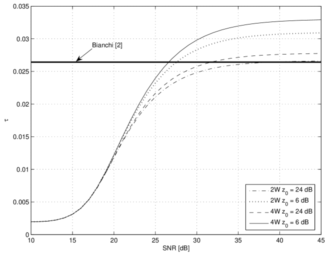
Figure 2: Theoretical behavior of the probability $\tau$ as a function of SNR for both 2 way (curves labelled 2W) and 4 way (curves labelled 4W) handshaking mechanisms. Curves have been obtained for the capture threshold $z_{0}$, payload size equal to 1024 bytes and for $N=20$ contending stations.

The theoretical behavior of the probabilities $\tau$, $P_{eq}$, and $P_{col}$ are depicted in Figs. 2 and 3 for both 2 way and 4 way hand-shaking mechanisms as a function of the channel SNR. All the curves have been drawn for $N=20$ contending stations and for a payload size equal to 1024 bytes. The curves have been parameterized with respect to the capture threshold $z_{0}$. A comparative analysis of the two figures reveals that for increasing values of the quality of the channel, as exemplified by the SNR, the transmission probability $\tau$ increases up to reaching a saturated level around $40$dB, above which the channel quality can be well assumed as ideal. Furthermore, this probability increases for lower values of the capture threshold $z_{0}$, i.e., for higher values of the capture probability.

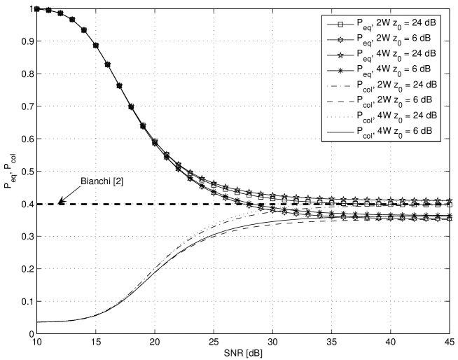
Figure 3: Theoretical behaviour of the equivalent failure transmission probability $P_{eq}$ as a function of SNR for both 2 way (curves labelled 2W) and 4 way (curves labelled 4W) handshaking mechanisms. Curves have been obtained for the capture threshold $z_{0}$, payload size equal to 1024 bytes and for $N=20$ contending stations.

A comparative analysis of the curves shown in Fig. 3 reveals that the equivalent transmission failure probability decreases for increasing values of SNR, achieving asymptotic values essentially equal to collision probability at high SNR values. Notice that the relation defining probability $\tau$ for the 2 way mechanism, as defined in (9), tends to the relation found by Bianchi [2]:

$$\tau=\frac{2(1-2p)}{(1-2p)(W+1)+pW(1-(2p)^{m})}$$

when $SNR\rightarrow\infty$, i.e., for $P_{e}(SNR)\rightarrow 0$, and $P_{cap}\rightarrow 0$. In this case, $P_{eq}\rightarrow p$, where $p$ is the collision probability as defined by Bianchi, and here identified by $P_{col}$. In this respect, our model is more general and also embraces Bianchi’s model as an asymptotic case. This is clearly highlighted in Figs. 2 and 3 whereby the Bianchi’s probabilities as specified in [2] are depicted as horizontal lines due to the independence of the Bianchi’s model on both capture effects and channel errors. On the other hand, for very low values of SNR, the equivalent failure probability $P_{eq}$ is practically 1 no matter what values are assumed by the other parameters.

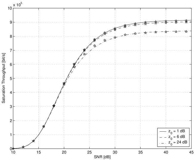
Figure 4: Saturation throughput for the 2 way mechanism as a function of the SNR, for three different capture thresholds $z_{0}$. Simulated points are identified by star-markers over the respective theoretical curves. Payload size is 1024 bytes, while the number of contending stations is $N=5$.

Fig. 4 shows the behavior of the saturation throughput for the 2 way mechanism as a function of the SNR, for three different capture thresholds, $z_{0}$, and for 5 transmitting stations. Simulated points are marked by star on the respective theoretical curves. As expected, throughput improves as the SNR increases up to 35 dB. Furthermore, throughput improves because of the capture effects.

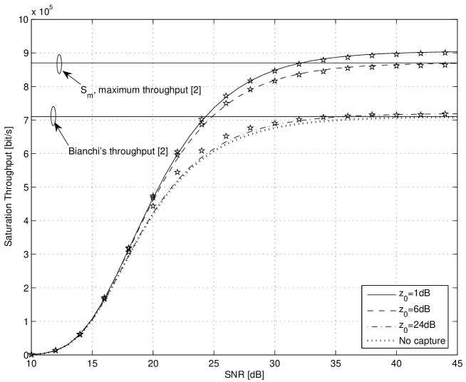
Figure 5: Saturation throughput for the 2 way mechanism as a function of the SNR, for three different capture thresholds $z_{0}$. Simulated points are identified by star-markers over the respective theoretical curves. Payload size is 1024 bytes, while the number of contending stations is $N=20$.

Fig. 5 shows the behavior of the saturation throughput for the 2 way mechanism as a function of the SNR, for three different capture thresholds, $z_{0}$, and for 20 transmitting stations. Upon comparing the curves shown in Fig.s 4 and 5, it is easily seen that capture effects allow the system throughput to be almost the same independently from the number of stations, since throughput curves related to $z_{0}=1$ dB are very close. On the other hand, when capture probability is low, i.e., for $z_{0}=24$dB, collision probability reduces the throughput as the number of contending stations increase.

With the aim of comparing the throughput predicted by the proposed model in a variety of transmission conditions to the Bianchi’s throughput, Fig. 5 also shows the Bianchi’s throughput along with the maximum throughput $S_{m}$ achievable upon optimizing the minimum contention window, $W$, as discussed in [2]. The maximum throughput evaluated by Bianchi is defined as:

$$S_{m}=\frac{E[PL]}{T_{s}+\sigma K+T_{c}\left(K(e^{1/K}-1)-1\right)}$$ (32)

whereby $K=\sqrt{\frac{T_{c}}{2\sigma}}$, while $T_{c}$ and $T_{s}$ are defined in (25) for the 2-way mechanism, and (17) for the 4-way mechanism. Notice that, as already suggested by Bianchi, $S_{m}$ is independent of the number $N$ of contending stations.

First of all, notice that as $SNR\rightarrow\infty$ and in absence of capture, the throughput predicted by our model tends to the Bianchi’s throughput, which also corresponds to about $z_{0}=24$dB, i.e., a transmission scenario in which capture threshold is so high that capture probability is very low. On the other hand, for decreasing values of $z_{0}$, throughput tends to increase, as expected, in the presence of capture. Secondly, for values of $z_{0}=6$dB, capture effects are such that the throughput reaches the value $S_{m}$ predicted by Bianchi under the hypothesis of employing an optimal minimum contention window size, even though in our simulation setup the minimum contention window is not chosen to be the optimal value yielding (32). For increasing values of capture probabilities, as exemplified by $z_{0}=1$dB, throughput goes above $S_{m}$. This is essentially due to the fact that capture tends to reduce the collision probability experienced by the stations which attempt to access the channel simultaneously, validating the key hypothesis suggested in (10). Indeed, simulation results confirm such a hypothesis.

In order to assess throughput performance as a function of the payload size, Fig. 6 shows throughput performance as a function of the SNR, for two different values of the payload sizes. Depending on the channel quality as exemplified by the SNR on the abscissa in Fig. 6, it could be preferable to transmit shorter packets for low SNRs. On the other hand, when channel quality improves, longer packets allow one to increase throughput.

Finally, Fig.s 7 and 8 show the behavior of the saturation throughput as a function of the number of the contending stations for 2 and 4 way mechanism, respectively, for various key values of the parameters SNR and $z_{0}$. In both figures, SNR$=\infty$ is used to signify ideal transmission (i.e., $P_{e}=0$), while $z_{0}=\infty$ means absence of capture effects. Notice that, as expected, in the 4 way mechanism, saturation throughput performance is less sensitive to capture effects. For comparison purposes, Fig.s 7 shows Bianchi’s throughput along with the maximum achievable throughput in (32). Notice that Bianchi’s throughput is superimposed on the curve labelled $SNR=\infty$ and $z_{0}=\infty$, as already noted from the simulation results shown in the previous figures. Achievable throughput in a variety of transmission conditions is usually less than $S_{m}$ in (32), specially when $SNR$ is lower than $45$dB: in this case, channel errors tend to dominate reducing the throughput. On the other hand, throughput can be higher than $S_{m}$ for a low number of contending stations (in the considered scenario, $N\leq 20$ contending stations) and for low values of capture thresholds $z_{0}$, say $z_{0}\leq 6$dB. On the other hand, employing the 4 way mechanism, throughput is very close to the theoretical Bianchi’s value $S_{m}=0.86$ Mbps no matter what the capture threshold $z_{0}$. This is due to the impact of the 4 way mechanism mitigating the effects of collisions between multiple contending stations.

VI Conclusions

In this paper, we provided an extension of the Markov model characterizing the DCF behavior at the MAC layer of the IEEE802.11 series of standards accounting for channel induced errors and capture effects typical of fading environments. The modelling allows taking into consideration the impact of channel contention in throughput analysis which is often not considered or it is considered in a static mode by using a mean contention period. Subsequently, based on justifiable assumptions, the stationary probability of the Markov chain is calculated to obtain the saturation throughput. The closed form expressions allow derivation of the throughput as a function of a multitude of system level parameters including packet and header sizes for a variety of applications. Simulation results confirm the validity of the proposed theoretical models.

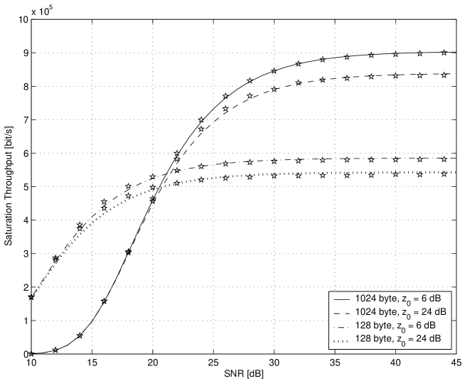
Figure 6: Saturation throughput for the 2 way mechanism as a function of the SNR, for payload sizes 128 and 1024 bytes, and $z_{0}=6,~{}24$ dB. Simulated points are identified by star-markers over the respective theoretical curves.

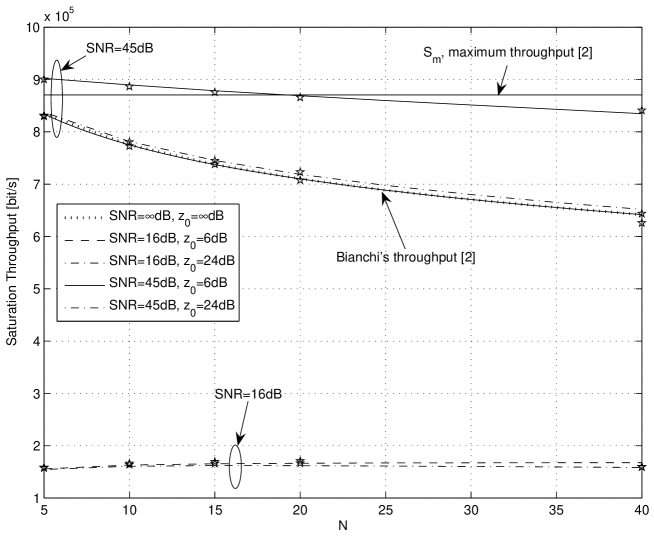
Figure 7: Saturation throughput for the 2 way mechanism as a function of the number of contending stations, for various values of the SNR and $z_{0}$ parameters. Payload size is 1024 bytes. Simulated points are identified by star-markers over the respective theoretical curves.

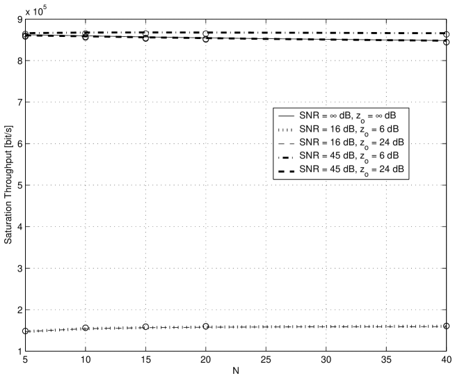
Figure 8: Saturation throughput for the 4 way mechanism as a function of the number of contending stations, for various values of the SNR and $z_{0}$ parameters. Payload size is 1024 bytes. Simulated points are identified by star-markers over the respective theoretical curves.

TABLE I: Typical network parameters

MAC header	24 bytes
PHY header	16 bytes
Payload size	1024 bytes
ACK	14 bytes
RTS	20 bytes
CTS	14 bytes
propagation delay $\tau_{p}$	1 $\mu s$
Slot time	20 $\mu s$
SIFS	10 $\mu s$
DIFS	50 $\mu s$
EIFS	300 $\mu s$
ACK timeout	300 $\mu s$
CTS timeout	300 $\mu s$

TABLE II: Throughput dependence on the per-station FER in a scenario with $N=9$ contending stations using the 2-way mechanism without capture. Packet size is $E[PL]=1024$ bytes.

FER	$S_{i}$ [Mbps]
$10^{-2},10^{-2},10^{-2}$	0.777
$10^{-2},10^{-3},10^{-4}$	0.781
$10^{-2},10^{-4},10^{-5}$	0.781
$10^{-3},10^{-3},10^{-3}$	0.784
$10^{-3},10^{-4},10^{-5}$	0.786
$10^{-3},10^{-5},10^{-6}$	0.785

References

- [1] IEEE Standard for Wireless LAN Medium Access Control (MAC) and Physical Layer (PHY) Specifications, November 1997, P802.11
- [2] G. Bianchi, ”Performance analysis of the IEEE 802.11 distributed coordination function”, IEEE JSAC, Vol.18, No.3, March 2000.
- [3] Jae Hyun Kim and Jong Kyu Lee ”Capture effects of wireless CSMA/CA protocols in Rayleigh and shadow fading channels”, IEEE Trans. on Veh. Tech., Vol.48, No.4, pp.1277-1286, July 1999.
- [4] M. Zorzi and R.R. Rao, ”Capture and retransmission control in mobile radio”, IEEE JSAC, Vol.12, No.8, pp.1289 - 1298, Oct. 1994.
- [5] Z. Hadzi-Velkov and B. Spasenovski, ”Capture effect in IEEE 802.11 basic service area under influence of Rayleigh fading and near/far effect”, In Proc. of 13th IEEE International Symposium on Personal, Indoor and Mobile Radio Communications, Vol.1, pp.172 - 176, Sept. 2002.
- [6] J.W. Robinson and T.S. Randhawa ”Saturation throughput analysis of IEEE 802.11e enhanced distributed coordination function”, IEEE JSAC, Vol.22, No.5, June 2004.
- [7] Z. Kong, D.H.K. Tsang, B.Bensaou, and D.Gao, ”Performance analysis of IEEE 802.11e contention-based channel access”, IEEE JSAC, Vol.22, No.10, Dec. 2004.
- [8] D. Qiao, S. Choi, and K.G. Shin ”Goodput analysis and link adaptation for IEEE 802.11a wireless LANs”, IEEE Trans. On Mobile Computing, Vol.1, No.4, Oct.-Dec. 2002.
- [9] P. Chatzimisios, A.C. Boucouvalas, and V. Vitsas, ”Influence of channel BER on IEEE 802.11 DCF”, IEE Electronics Letters, Vol.39, No.23, pp.1687-1689, Nov. 2003.
- [10] Wei Zhuang, Yung-Sze Gan, Kok-Jeng Loh, and Kee-Chaing Chua, ”Policy-based QoS-management architecture in an integrated UMTS and WLAN environment”, IEEE Communications Magazine, Vol.41, No.11, pp.118-125, Nov. 2003.
- [11] W. Liu, W. Lou, X. Chen, and Y. Fang, ”A QoS-enabled MAC architecture for prioritized service in IEEE 802.11 WLANs”, Proc. IEEE GLOBECOM’03, Vol.7, pp.3802-3807, Dec. 2003.
- [12] G. Fodor, A. Eriksson, and A. Tuoriniemi, ”Providing quality of service in always best connected networks”, IEEE Communications Magazine, Vol.41, No.7, pp.154-163, July 2003.
- [13] J. Zhao, Z. Guo, Q. Zhang, and W. Zhu, ”Performance study of MAC for service differentiation in IEEE 802.11”, In Proc. of IEEE GLOBECOM’02, Vol.1, pp.778-782, Nov. 2002.
- [14] W. Pattara-Atikom, P. Krishnamurthy, and S. Banerjee, ”Distributed mechanisms for quality of service in wireless LANs”, IEEE Personal Communications, Vol.10, No.3, pp.26-34, June 2003.
- [15] Ye Ge and J. Hou, ”An analytical model for service differentiation in IEEE 802.11”, Proc. ICC ’03, Vol.2, pp.1157-1162, May 2003.
- [16] H. L. Truong and G. Vannuccini, ”Performance evaluation of the QoS enhanced IEEE 802.11e MAC layer”, In Proc. of IEEE VTC 2003-Spring, Vol.2, pp.940-944, April 2003.
- [17] Q. Li and M. VanderSchaar, ”Providing adaptive QoS to layered video over wireless local area networks through real-time retry limit adaptation”, IEEE Trans. on Multimedia, Vol.6, No.2, pp.278-290, April 2004.
- [18] Q. Zhang, C. Guo, Z. Guo, and W. Zhu, ”Efficient mobility management for vertical handoff between WWAN and WLAN”, IEEE Communications Magazine, Vol.41, No.11, pp.102-108, Nov. 2003.
- [19] H. Honkasalo, K. Pehkonen, M. T. Niemi, and A.T. Leino, ”WCDMA and WLAN for 3G and beyond”, IEEE Personal Communications, Vol.9, No.2, pp.14-18, April 2002.
- [20] S. Park, K. Kim, D.C. Kim, S. Choi, and S. Hong, ”Collaborative QoS architecture between DiffServ and 802.11e wireless LAN”, In Proc. of IEEE VTC 2003-Spring, Vol.2, pp.945-949, April 2003.
- [21] F. Daneshgaran and M. Laddomada, “Reduced complexity interleaver growth algorithm for turbo codes,” IEEE Trans. on Wireless Communications, vol.4, no.3, pp.954-964, May 2005.
- [22] F. Daneshgaran, M. Laddomada, and M. Mondin, “Interleaver design for serially concatenated convolutional codes: Theory and application,” IEEE Trans. on Information Theory, Vol.50, No. 6, pp. 1177-1188, June 2004.
- [23] Proakis, J. G., “Digital Communications,” McGraw Hill, Fourth Edition, New York, 2001.
- [24] F. Daneshgaran, M. Laddomada, and M. Mondin, “An extensive search for good punctured rate k/k+1 recursive convolutional codes for serially concatenated convolutional codes,” IEEE Trans. on Inform. Theory, vol.50, no.1, pp.208-217, January 2004.
- [25] F. Daneshgaran, M. Laddomada, and M. Mondin, “High rate recursive convolutional codes for concatenated channel codes,” IEEE Trans. on Communications, vol.52, no.11, pp.1846-1850, Nov. 2004.
- [26] M.K. Simon and M. Alouini, Digital Communication over Fading Channels: A Unified Approach to Performance Analysis, Wiley-Interscience, 1st edition, 2000.
- [27] T. Rappaport, Wireless Communications, Prentice Hall, 1999.
-
[28]
Wu Xiuchao, ”Simulate 802.11b Channel within NS-2”, available
online at
http://www.comp.nus.edu.sg/~wuxiucha/research/reactive/report/80211ChannelinNS2_new.pdf