A Unified Model of $\alpha$-Helix/$\beta$-Sheet/Random-Coil Transition in Proteins

Abstract

The theory of transition between $\alpha$-helix, $\beta$-sheet and random coil conformation of a protein is discussed through a simple model, that includes both short and long-range interactions. Besides the bonding parameter and helical initiation factor in Zimm-Bragg model, three new parameters are introduced to describe beta structure: the local constraint factor for a single residue to be contained in a $\beta$-strand, the long-range bonding parameter that accounts for the interaction between a pair of bonded $\beta$-strands, and a correction factor for the initiation of a $\beta$-sheet. Either increasing local constraint factor or long-range bonding parameter can cause a transition from $\alpha$-helix or random coil conformation to $\beta$-sheet conformation. The sharpness of transition depends on the competition between short and long-range interactions. Other effective factors, such as the chain length and temperature, are also discussed. In this model, the entropy due to different ways to group $\beta$-strands into different $\beta$-sheets gives rise to significant contribution to partition function, and makes major differences between beta structure and helical structure.

I Introduction

The formation of protein secondary structure has attracted great interest in the past 50 years, due to their remarkably regular spatial arrangementBT . There are usually two distinct interactions involved: namely short-range interaction between atoms and groups which are near neighbors in sequence along the chain; and long-range interactions involving pairs of units which are remote in sequence but near in spaceFlory . How these interactions affect the formation of secondary structure, especially $\beta$-sheet, is essential in the study of protein folding. On the other hand, a protein sequence can display structure ambivalence and interconverts between $\alpha$-helix and $\beta$-sheet conformationsPatel:07 . This phenomenon may concern about many well-known diseases, such as Alzheimer’s, Mad Cow and Parkinson’s disease. But the underlying mechanism is still not very clear. In this paper, we try to establish a unified statistical model of $\alpha$-helix/$\beta$-sheet/random-coil transition in proteins, which includes both short-range and long-range interactions. It will be an extension of Zimm-Bragg’s (Z-B) model to include beta structures as wellZB , and is totally different from former tension-induced $\alpha$/$\beta$ transition theoryBirstein ; David1 ; David2 ; Schor ; Finkelstein , which has only mentioned short-range interactions.

$\alpha$-helix and $\beta$-sheet are most important secondary structure elements in protein. An $\alpha$-helix is found when a stretch of consecutive residues all have torsion angle pair $(\phi,\psi)$ approximately $-60^{o}$ and $-50^{o}$, the allowed region in the bottom left quadrant of the Ramachandran plot. In $\alpha$-helix, the CO group of residue $n$ is bonded to the NH group of residue $n+4$. Thus, it contains only short-range interactions. The $\beta$-sheet, however, is built up of several segments of the polypeptide chain. And long-range interactions are involved. These segments, $\beta$-strands, are usually of $5\sim 10$ residues long, with $(\phi,\psi)$ angles in the broad structurally allowed region in the upper left quadrant of the Ramachandran plot. The $\beta$-strands are aligned adjacent to each other, such that hydrogen bonds can form between CO groups of one strand and NH group of an adjacent strand, and vice versa.

In the presence of long-range interactions, it is not sufficient to distinguish states of a protein by only identifying the states of each amino acid. Various bonding patterns of $\beta$-strands can result in different states. Therefore, the different ways of arranging $\beta$-strands into $\beta$-sheets have to be considered. In this paper, we will establish a model, in which two sets of codes are introduced to represent respectively the state of each residue and connecting pattern of the $\beta$-strands. Accordingly, we are able to write down the partition function, through which the transition between alpha, beta and random coil structures of a protein is discussed in detail.

When no $\alpha$-helix is presented, our model shows that a coil-to-sheet transition occurs as the local constraint factor is increased. And the sharpness of transition is determined by the long-range bonding parameter and the initiation factor. The smaller these two parameters are, the sharper the transition will be. This result has similar feature as that in coil-to-helix transition, which has been studied extensively by Z-B model. With the increment of the local constraint factor, the normalized number of $\beta$-strands increases firstly, and then decreases after passing the transition point, due to the competition between short-range and long-range interactions.

Helix/sheet transition is of great interest in this paper. In the presence of long-range interactions, the entropy contribution to partition function becomes more important. This is due to the ways of connecting $\beta$-strands into $\beta$-sheets can be various, even when the state of each residue is known. Unlike enthalpy controlled helix/coil transition in Z-B model, helix/sheet transition is driven by entropy. A transition from $\alpha$-helix to $\beta$-sheet occurs, when either the local constraint factor of beta residues or the long-range bonding parameter of $\beta$-stands is increased. The sharpness of transition depends on the competition between short-range and long-range interactions. Moreover, the compromise between short-range and long-range interactions is able to give rise to mixed $\alpha/\beta$ structure.

The length and temperature dependence of the transition are also studied. Statistical study of protein structures reported in Protein Data Bank (PDB) shows that the fractions of alpha and beta residues are nearly unchanged when the chain is sufficiently long($n\geq 50$). Comparing our theoretical result with the data, we are able to identify the values of parameters in our model. Interestingly, the parameter values are close to the transition point. This indicates that protein sequences in living cells are well selected by evolution, to compromise the required properties such as stability, flexibility and diversity. The temperature dependence is studied based on above parameter values. Our results show that at low temperature, $\alpha$-helix is dominated because of strong local interactions; while at high temperature, beta structure is more favored due to larger entropy contribution.

This paper will begin with an extension of Z-B model in Section II, where connection properties of $\beta$-strands are introduced to obtain a complete description for the state of a protein. The partition function is obtained in Section III, by simple assumptions on the states of amino acid residues and $\beta$-strands. In Section IV, we discuss the transition from random coil and $\alpha$-helix to $\beta$-sheet under different conditions. At last, a brief conclusion is given in Section V.

II Model

This section presents a model for the polypeptide chain that is intended to extend Z-B model to include beta structures. Specifically, it establishes a second order coding for the connection of $\beta$-strands in $\beta$-sheets. The partition function is then formulated as contributions from all $\alpha$, all $\beta$ and $\alpha/\beta$ mixed structures. To describe the model in detail, we firstly have to make a complete description of the conformation of a chain, which will be finished in two steps.

The first step is to define the state of each amino acid residue, in other words, which one is $\alpha$-helical and which one is in $\beta$-strand. Definition of $\alpha$-helical residue is straightforward, i.e., those residues whose NH group is bonded to the CO group of the fourth preceding residue. Here we have assumed that bonding of a residue, if it occurs in $\alpha$-helix, is always to the fourth preceding residue, and disregard other helical structures such as $\pi$-helix or $3_{10}$-helixRohl . To determine whether a residue is in $\beta$-strand is sticky and depends on the state of its neighboring residues. We assume that a residue is regarded as in $\beta$-strand if the angle pair $(\phi,\psi)$ of itself or both of its neighboring residues take values in the upper left quadrant of Ramachandran plot. Now, a chain of $n$ residue can be described by a sequence of $n$ symbols, each of which can have one of three values: digit $0$ represents a random coil residue, $1$ for an $\alpha$-helical residue, and $2$ for a residue in $\beta$-strand. An example is shown by the 1st code in Fig. 1.

Knowing the state of each residue is not sufficient. We need a 2nd code to describe how $\beta$-strands are connected into $\beta$-sheets. We assign a symbol $S_{i}^{j}$ for the $j$’th strand in the $i$’th $\beta$-sheet(2nd code in Fig. 1). Here, the number $j$ is assigned not according to the sequence along the chain, but the spatial connection position in the $\beta$-sheet. Now, the state of a chain can completely be described by these two sequences of codes as shown in Fig. 1. We will see later that this second step makes major differences between $\beta$-sheet and $\alpha$-helix, and gives rise to the helix/sheet transition.

Peptide units:	1	2	3	4	5	6	7	8	9	$\cdot$	$\cdot$	$\cdot$
1st code:	0	0	0	0	0	1	1	1	1	0	0	0	0	2	2	2	2	2	2	0	0	0	0	0	2	2	2	2	2	0	0	0	0	0	2	2	2	2	2	0	0	$\cdots$
Weights:	1	1	1	1	1	$\sigma s$	$s$	$s$	$s$	1	1	1	1	$w$	$w$	$w$	$w$	$w$	$w$	1	1	1	1	1	$w$	$w$	$w$	$w$	$w$	1	1	1	1	1	$w$	$w$	$w$	$w$	$w$	1	1	$\cdots$
2nd code:														$S_{1}^{1}$											$S_{1}^{2}$										$S_{2}^{1}$							$\cdots$
Weights:														$\eta p$											$p$										$\eta p$							$\cdots$

Figure 1: Coding and weight of residues in a chain.

Finally, we introduce the statistical weight for a given state of a chain as the product of following factors, according to the coding established above:

1. The quantity unity for every $0$ (coil residue).

2. The quantity $s$ for every $1$ that follows a $1$ (helical residue).

3. The quantity $\sigma s$ for every $1$ that follows $\mu$ or more 0’s (initiation of a helix).

4. The quantity $w$ for every $2$ (residue in a $\beta$-strand).

5. The quantity $p$ for every $S_{i}^{j}$ with $j\geq 2$ ($\beta$-strand).

6. The quantity $\eta p$ for every $S_{i}^{1}$ (initiation of a $\beta$-sheet).

7. The quantity $0$ for one of the following cases:

   1. every $1$ that follows $2$ or a number of $0$ less than $\mu$;

   2. every $2$ that follows $1$ or a number of $0$ less than $\mu$;

   3. every single $2$ between two $0$.

The effect of assumption (7) is that the secondary structures are separated from each other by at least $\mu$ coil residues; and each $\beta$-strand contains at least $2$ residues. The number $\mu$ is varied from case to case. For example, two helices are separated by at least $4$ residues, while two $\beta$-strands can be separated by only two residues ($\beta$-turn). In this paper, we will take a uniform value, say $\mu=3$, for simplicity. We will see later that the value of $\mu$ has little effect on the transition, especially for long chains.

The meaning of the statistical weights are as follows. The first three weights are the same as those in Z-B modelQian ; Poland . The factor unity is arbitrarily assigned to coil residues, since only the relative ratio is effective. The factor $s$ measures the contribution of a helical residue, relative to a coil residue, to the partition function. It contains a decrease due to restriction of torsion angle and an enhancement because of the hydrogen bonding. The factor $\sigma$ represents the decrease of weight $s$ for the first unit in a helix, since the formation of first hydrogen bond causes restriction of the freedom of residues between the bonded ones.

The next three weights are new and for beta structures. The factor $w$ measures the contribution of a residue in $\beta$-strand, relative to a coil residue, to the partition function. It contains an slight increase due to the lower energy compared to coil residuesFlory . Note the torsion angle of beta residues can take values from a quite broad region from the upper left quadrant of the Ramachandran plot, thus the restriction in freedom is not serious. The factor $p$ represents long-range interactions between a pair of bonded $\beta$-strands. This includes a decrease due to restriction of freedom of residues between the two bonded $\beta$-strands, and an enhancement due to the hydrogen bonding. Nevertheless, since two $\beta$-strands can be separated by long distance along the chain, the effect of decreasing is dominant. Therefore, the value of $p$ is usually small. Similar to the case of helix, an initiation factor $\eta$ is introduced to measure the decrease of weight $p$ for the first pair of $\beta$-strands in a $\beta$-sheet. In summary, for the five weights in the model, the factors $s$ and $w$ are usually sightly larger than unity, while $\sigma$, $p$ and $\eta$ are all less than unity.

In the above discussion, we assume that the bonding energy(factor $p$) of each pair of $\beta$-strands are the same, and independent of the number of both residues and hydrogen bonds between the bonded $\beta$-strands. It is a highly simplified representation of the problem and enables us to write down the partition function. One may introduce a set of factors $p(n_{1},n_{2})$, which depends on those two values, to make the model more realistic. But since bonding patterns of $\beta$-sheet varies greatly, our present knowledge is too incomplete to justify a more refined model.

III Mathematical treatment

A formal representation of partition function $Z$ for a chain of $n$ residues can be obtained from above model by direct enumerating of the number of different ways of arranging digits $0,1,2$ and the state of strands $S_{i}^{j}$.

Let $X=(n_{a},n_{b},l_{b},l_{b},k_{b})$ be the state of a chain, where $n_{a}$, $n_{b}$, $l_{a}$, $l_{b}$, $k_{b}$ are respectively the number of helical residues, beta residues, $\alpha$-helices, $\beta$-strands and $\beta$-sheets. Then the statistical weight of state $X$ is given by

$$Q(X)=s^{n_{a}}w^{n_{b}}\sigma^{l_{a}}p^{l_{b}}\eta^{k_{b}}.$$ (1)

Let $S(X)$ be the number of states, which has the same statistical weight as $X$, and $\Omega$ be the phase space of possible states, then the partition function is represented as

$$Z=\sum_{X\in\Omega}Q(X)S(X).$$ (2)

Explicitly, the phase space $\Omega$ is given by

$$\Omega=\left\{X\in\mathbb{Z}^{5}:\ \ \ \begin{array}[]{l}0\leq k_{b}\leq l_{b}/2\leq n_{b}/4\leq\lfloor\frac{n}{4+2\mu}\rfloor,\\ 0\leq l_{a}\leq n_{a}\leq\lfloor\frac{n}{1+\mu}\rfloor,\\ n-(n_{a}+n_{b})\geq\mu(l_{a}+l_{b})\\ l_{b}=n_{b}=0\ \ \mathrm{if}\ k_{b}=0\\ n_{a}=0\ \ \mathrm{if}\ l_{a}=0\end{array}\right\}.$$

The degeneracy $S(X)$ is formulated as

$$\begin{array}[]{rcl}S(X)&=&C_{n_{a}-1}^{l_{a}-1}C_{n_{b}-l_{b}-1}^{l_{b}-1}C_{l_{b}-k_{b}-1}^{k_{b}-1}\\ &&\times C_{n-n_{a}-n_{b}-(\mu-1)(l_{a}+l_{b})}^{l_{a}+l_{b}}C_{l_{a}+l_{b}}^{l_{a}}.\end{array}$$ (3)

This formula is obtained by following steps. Firstly, we partition $n_{a}$ amino acids into $l_{a}$ $\alpha$-helices, $n_{b}$ amino acid into $l_{b}$ $\beta$-strands and $l_{b}$ $\beta$-strands into $k_{b}$ $\beta$-sheet along the chain. Then we insert $n-n_{a}-n_{b}$ coil residues between $\alpha$-helices and $\beta$-strands. Finally, we rearrange the order of $\alpha$-helices and $\beta$-strands. The meaning of each term is explained as follows. The binomials $C_{n_{a}-1}^{l_{a}-1}$ represents the number of ways to group $n_{a}$ helical residues into $l_{a}$ helices. The terms $C_{n_{b}-l_{b}-1}^{l_{b}-1}$ and $C_{l_{b}-k_{b}-1}^{k_{b}-1}$ are similar, representing the number of ways to group beta residues into $\beta$-strands and $\beta$-strands into $\beta$-sheets, respectively. Here each $\beta$-sheet has at least two strands; and each $\beta$-strand has at least two residues. The binomial $C_{n-n_{a}-n_{b}-(\mu-1)(l_{a}+l_{b})}^{l_{a}+l_{b}}$ represents how many ways to insert $n-n_{a}-n_{b}$ coil residues between the secondary structure elements, such that consecutive helix and strand are separated by at least $\mu$ coil residues. The last factor $C_{l_{a}+l_{b}}^{l_{b}}$ represents how many ways to arrange the order of $\alpha$-helices and $\beta$-strands. Note that here the $\alpha$-helices are considered as identical. The $\beta$-strands are assumed to connect to only the neighboring ones. Long-distance connections in $\beta$-sheets are neglected, since the usual adopted arrangements are quite limited at room temperature. One may propose other assumptions. For example, $\beta$-strands are assumed to be able to connect to each other freely ($l_{b}!C_{l_{a}+l_{b}}^{l_{b}}$), despite their length and distance. Or all $\alpha$-helices and $\beta$-strands are considered as distinguishable ($(l_{a}+l_{b})!$), in case of very strong long-range interactions between secondary structure elements. Different assumptions may give different results, but the general property of transition is almost unchanged, according to our simulations. Further discussions are shown in the appendix.

The partition function can be rewritten according to the structure of the chain as follows:

$$Z=1+Z_{\alpha}+Z_{\beta}+Z_{\alpha/\beta}$$ (4)

where

$$Z_{\alpha} = \sum_{l_{a}=1}^{\lfloor\frac{n}{1+\mu}\rfloor}\sigma^{l_{a}}\sum_{n_{a}=l_{a}}^{n-\mu l_{a}}s^{n_{a}}C_{n_{a}-1}^{l_{a}-1}C_{n-n_{a}-(\mu-1)l_{a}}^{l_{a}}$$ (5)

$$Z_{\beta} = \sum_{k_{b}=1}^{\lfloor\frac{n}{4+2\mu}\rfloor}\eta^{k_{b}}\sum_{l_{b}=2k_{b}}^{\lfloor\frac{n}{2+\mu}\rfloor}p^{l_{b}}C_{l_{b}-k_{b}-1}^{k_{b}-1}$$ (6)

$${}\times\sum_{n_{b}=2l_{b}}^{n-\mu l_{b}}w^{n_{b}}C_{n_{b}-l_{b}-1}^{l_{b}-1}C_{n-n_{b}-(\mu-1)l_{b}}^{l_{b}}$$

$$Z_{\alpha/\beta} = \sum_{k_{b}=1}^{\lfloor\frac{n}{4+2\mu}\rfloor}\eta^{k_{b}}\sum_{l_{b}=2k_{b}}^{\lfloor\frac{n}{2+\mu}\rfloor}p^{l_{b}}C_{l_{b}-k_{b}-1}^{k_{b}-1}$$

$${}\times\sum_{n_{b}=2l_{b}}^{n-\mu l_{b}}w^{n_{b}}C_{n_{b}-l_{b}-1}^{l_{b}-1}\sum_{l_{a}=1}^{\lfloor\frac{n-n_{b}-\mu l_{b}}{1+\mu}\rfloor}\sigma^{l_{a}}C_{l_{a}+l_{b}}^{l_{a}}$$

$${}\times\sum_{n_{a}=l_{a}}^{n-n_{b}-\mu(l_{a}+l_{b})}s^{n_{a}}C_{n_{a}-1}^{l_{a}-1}C_{n-n_{b}-n_{a}-(\mu-1)(l_{a}+l_{b})}^{l_{a}+l_{b}}$$

Here $Z_{\alpha}$ (or $Z_{\beta}$) represents the partition function for the states of all $\alpha$ (or $\beta$) structures, and $Z_{\alpha/\beta}$ for $\alpha/\beta$ mixed structures.

In the following, we will show how the $\alpha$-helix, $\beta$-sheet and random coil conformation at equilibrium state transit to each other, when the parameters are changing. We define the fraction of helical and beta residues respectively as

$$\theta_{a}:=\frac{n_{\alpha}}{n}=\frac{1}{n}\dfrac{\partial\ln Z}{\partial\ln s},\;\theta_{b}:=\frac{n_{\beta}}{n}=\frac{1}{n}\dfrac{\partial\ln Z}{\partial\ln w}.$$ (8)

The normalized number of $\alpha$-helices and $\beta$-strands are also of interest.

$$\phi_{a}:=\frac{l_{\alpha}}{n}=\frac{1}{n}\dfrac{\partial\ln Z}{\partial\ln\sigma},\;\phi_{b}:=\frac{l_{\beta}}{n}=\frac{1}{n}\dfrac{\partial\ln Z}{\partial\ln p}.$$ (9)

IV Results and Discussions

From discussions in previous section, it is easy to show that in the absence of long-range interaction, the partition function($Z=1+Z_{\alpha}$) is the same as that for helix/coil transition, which has been well studied by Z-B model. In following, we will focus on how the parameters induce transitions between $\alpha$-helix, $\beta$-sheet and random coil. From (5)-(III), the parameter $\mu$ has only minor effect on the results. Here, we will set $\mu=3$ for the minimum number of coil residues between secondary structures.

IV.1 Sheet/Coil Transition

At first, we study the transition from random coil to regular $\beta$-sheet($Z=1+Z_{\beta}$), which is similar to helix/coil transitionZB ; Birshtein; Grosberg .

In this case, We have three tuneable parameters: $w$ for local constraint of single residue, $p$ for long-range bonding interactions between a pair of bonded $\beta$-strands and $\eta$ for initiation correction of a $\beta$-sheet. The dependence of $\theta_{b}$ and $\phi_{b}$ on the parameters are shown at Fig. 2.

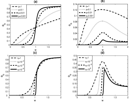
Figure 2:  Sheet/coil transition ($n=200$). The dependence of $\theta_{b}$ (a) and $\phi_{b}$ (b) on $w$, with different values of $p$, and $\eta$ is set to $1.0$. The dependence of $\theta_{b}$ (a) and $\phi_{b}$ (d) on $w$, with different values of $\eta$, and $p$ is set to $0.01$.

From Fig. 2(a), 2(c), we can see that when $w$ is increasing, the fraction of beta residues $\theta_{b}$ goes from zero to unity monotonously. This means the random coils turn into regular $\beta$-sheets when the local interactions become stronger. This transition usually happens at $w=1$, in accordance with Z-B model. The sharpness of transition depends on $p$ and $\eta$. The smaller $p$ or $\eta$ is, the sharper the transition will be.

Unlike the fraction of $\beta$ residues, which increases monotonously with respect to $w$, the number of $\beta$-strands increases firstly to reach a peak at around the transition point, and then decreases when $w$ keeps increasing (Fig. 2(b),(d)). We argue that this is a consequence of the competition between short and long-range interactions. Generally speaking, when $w$ is less than unity, short-range interactions prompt long-range interactions. With the increment of $w$, there tends to be more $\beta$-strands, as well as the strands get longer. Thus $\theta_{b}$ and $\phi_{b}$ increase simultaneously. When $w$ is larger than unity, short-range interactions suppress long-range interactions. As a consequence, when $w$ is increasing further, $\theta_{b}$ is almost unchanged while $\phi_{b}$ drops continuously. It means that there tends to be less $\beta$-strands and the strands still grow longer and longer.

IV.2 Helix/Sheet Transition

A more interesting result is $\alpha$-helix/$\beta$-sheet transition. Since the major difference of $\beta$-sheet from $\alpha$-helix is the existence of long-range interaction, which is described by parameters $p$ and $\eta$. Thus not only the increase of local effect $w$, but also the increment of long-range interaction parameters $p$ and $\eta$ can induce a transition from helical structure to beta structure(Fig. 3).

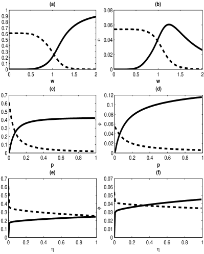
Figure 3:  Helix/sheet transition ($n=200$). In (a)(c)(e), the dashed lines are for $\theta_{a}$; while the solid lines are for $\theta_{b}$. In (b)(d)(f), the dashed lines are for $\phi_{a}$; and the solid lines are for $\phi_{b}$. (a) The dependence of $\theta_{a}$, $\theta_{b}$ on $w$. (b) The dependence of $\phi_{a}$, $\phi_{b}$ on $w$. (c) The dependence of $\theta_{a}$, $\theta_{b}$ on $p$. (d) The dependence of $\phi_{a}$, $\phi_{b}$ on $p$. (e) The dependence of $\theta_{a}$, $\theta_{b}$ on $p$. (f) The dependence of $\phi_{a}$, $\phi_{b}$ on $p$. In all computations, the chain length is $n=200$. The parameters used are, except particular indicated, $s=1.15$, $\sigma=0.037$, $w=1.03$, $p=0.072$ and $\eta=1$.

From Fig. 3(a,b), we can see that $\alpha$-helices transit to $\beta$-sheets with the increment of short-range interaction $w$. When $w$ is further increasing, the short-range interaction takes over long-range interactions, and therefore the normalized number of $\beta$-strands $\phi_{b}$ decreases.

From Fig. 3(c)-(e), we can see that the fraction of beta structure is very sensitive to the long-range interactions ($p$ and $\eta$) when the parameters are small ($p,\eta\ll 1$). This is a consequence of large entropy and high cooperativity of beta structures. Yet when the long-range interactions are strong enough ($p,\eta\sim 1$), the dependence of $\theta$ and $\phi$ on the parameters are far less evident.

In the present of long-range interactions, the entropy contribution to the partition function become important. This is originated from two sources: different methods of arranging secondary structure segments along the chain; and the ways of connecting $\beta$-strands into $\beta$-sheets, which is specified for beta structure. In protein, helical structure tends to have lower energy due to local hydrogen bonds, while the beta structure has larger entropy. As consequence, coil/helix transition is enthalpy controlled, while helix/sheet transition is entropy driven. Moreover, the longer the chain is, the sharper the helix/sheet transition will be. This helix/sheet transition picture may shed light on the mechanisms of structure transition of prionPrusiner and other proteinsPatel:07 .

IV.3 Length Dependence

The length dependence of the average fractions of alpha and beta residues obtained by studying the native structures in Protein Data Bank is plotted in Fig. 4. The results show that despite the variety from one protein to another, the average fractions are roughly independent to the chain length, except for very short chains ($n\leq 30$), with about $32\%$ alpha residues and $25\%$ beta residues. The data can be fitted by our model with parameters $w=1.03,p=0.072,\eta=1,s=1.15,\sigma=0.037$ (Fig. 4 (a)). Note that here the number of alpha residues from our model is given by $n_{\alpha}=n(\theta_{a}+3\phi_{a})$. Since in our model, the first three residues in every helix is not treated as helical. The same set of parameters also gives good agreement for the average number of $\alpha$-helices and $\beta$-strands(Fig. 4(b)). Accordingly, we obtain the average length of $\alpha$-helix to be $11$, and $\beta$-strand to be $6$, both agree with experimental data.

In previous simulation results(Fig. 3), we can see that while fitting our model to PDB data, the parameters take values around the helix/sheet transition point. We argue that this is not by chance, but is a prerequisite for proteins in living cells. Since diverse structure of proteins in living cells is required for their biological functions, particular values of the parameters are needed to compromise the required properties such as stability, flexibility and diversity, by natural selection.

(a)

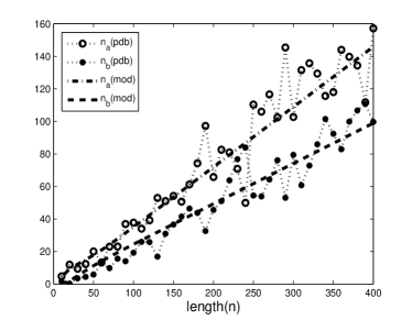
(b)

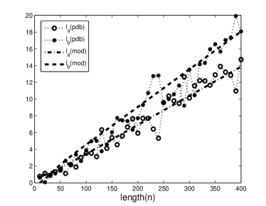
Figure 4:  Experimental data and theoretical simulation for the length dependence. The data are fitted by the model with parameters $w=1.03,p=0.072,\eta=1,s=1.15,\sigma=0.037$. (a) The average number of alpha and beta residues. (b) The average number of $\alpha$-helices and $\beta$-strands.

IV.4 Temperature Dependence

From previous discussion, helical structure tends to have low enthalpy, and beta structure tends to have large entropy. Thus, under certain condition, we should have a transition from helical structure to beta structure when the temperature is increased. To study this temperature induced transition, we need to explore the dependence of parameters on temperature. For the parameter $s$, for instance, we haveLR

$$s=\exp(\Delta G/k_{B}T)$$

where $T$ is the temperature. Here $\Delta G$ is the free energy change by converting one residue from random coil state to helical state. Assume that $\Delta G$ is independent to the temperature. Then the parameters $s_{i}$ for corresponding temperatures $T_{i}$ ($i=0,1$) are related by

$$s_{1}=s_{0}^{r}$$

where $r=T_{0}/T_{1}$ is the ratio of original and final temperature. Let $T_{0}=300K$ be the room temperature, thus we can investigate the temperature induced structure transition by changing the system parameters simultaneously

$$(\sigma,s,\eta,w,p)\rightarrow(\sigma^{r},s^{r},\eta^{r},w^{r},p^{r})$$

with $r=T/T_{0}$. The simulation results are shown in Fig. 5.

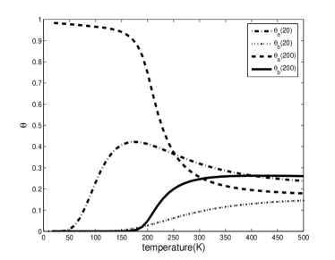
Figure 5:  Temperature dependence of fractions of alpha and beta resides for both short ($n=20$) and long ($n=200$) chains. Here $T_{0}=300K,w=1.03,p=0.072,\eta=1,s=1.15,\sigma=0.037$.

The transition from alpha to beta structure, when the temperature is increasing, is obvious in our simulation. For long chains, at low temperature, $\alpha$-helix is dominated because of strong local interactions; while at high temperature, beta structure is more favored for larger entropy contribution. But for short chains ($n<=26$ in this case), $\alpha$-helix becomes unstable at low temperature, and $\theta_{a}$ drops to zero. A big drawback of the results in Fig. 5 is that the regular secondary structures will not break into random coils at high temperature, by which the proteins should unfold. This is mainly due to our strong assumption that $\Delta H$ does not change with the temperature, which is not true when the temperature is far from the room temperature.

V Conclusion

In this paper, we extend the Z-B model to include beta structures, by introducing two sets of codes which represent respectively the state of each amino acid residue and connecting pattern of the $\beta$-strands. In additional to the bonding parameter and helical initiation factor in Z-B model, three new parameters are introduced to describe beta structures: the local constraint factor for a single residue to be contained in a $\beta$-strand, the long-range bonding parameter that accounts for the interaction between a pair of bonded $\beta$-strands, and a correction factor for the initiation of a $\beta$-sheet. Then the partition function is obtained based on our model, which contains both short and long-range interactions.

Through numerical study, the transition from random coil and $\alpha$-helical conformation to $\beta$-sheet structure are discussed respectively. In common, either the increase of the short-range or the long-range interactions of beta structure can cause a transition. And the sharpness of transition is mainly determined by the long-range bonding parameter and the initiation factor. However, the coil/sheet transition is enthalpy controlled, while helix/sheet transition is entropy driven. Other effective factors, such as the chain length and temperature, are also shown. The PDB data for protein chains with different length are fitted by our model and show a fairly well agreement. In this way, we can identify the values of parameters in our model. Interestingly, these values are close to the transition point. This indicates that protein sequences in living cells are well selected by evolution, to compromise the required properties such as stability, flexibility and diversity. At last, by considering the relationship between statistical weights and free energy, a temperature induced helix/sheet transition is observed. Our results show that at low temperature, $\alpha$-helix is dominated because of strong local interactions; while at high temperature, beta structure is more favored due to large entropy contribution.

We hope our results may shed light on the mechanisms of structure transition in prion and other proteins, as well as the understanding of short and long-range interactions in the formation of secondary structures.

Appendix A

The exact factor for different ways of arranging $\alpha$-helices and $\beta$-strands is undetermined in our present model, since our current knowledge about the secondary structure arrangement in natural proteins is too incomplete to justify the models. In general, we have three extreme cases. If the connections are highly restricted, i.e., $\beta$-strands are assumed to connect to only the neighboring ones, the factor $C_{l_{a}+l_{b}}^{l_{b}}$ would be a good estimate (Case $A_{1}$). On the other extreme, if the $\beta$-strands can connect to each other freely, despite their long distance along the chain, the factor should be $l_{b}!C_{l_{a}+l_{b}}^{l_{b}}$ (Case $A_{2}$). But this can only happen at very high temperature. Moreover, we can even assume that all $\alpha$-helices and $\beta$-strands are distinguishable, in case of very strong long-range interactions between secondary structure elements. Then the factor will be $(l_{a}+l_{b})!$ (Case $A_{3}$). Different assumption may give different results, but the general properties of transition are almost unchanged, which is shown in Fig. 6.

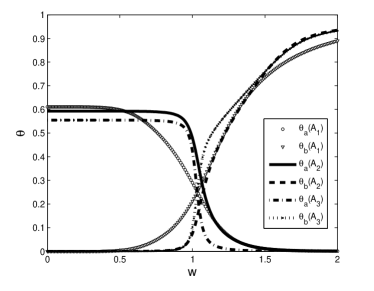
Figure 6:  Comparison of helix/sheet transition under three different assumptions. Case $A_{1}$ with $s=1.15$, $\sigma=0.037$, $p=0.072$ and $\eta=1$. Case $A_{2}$ with $s=1.14$, $\sigma=0.04$, $p=0.0062$ and $\eta=1$. Case $A_{3}$ with $s=1.14$, $\sigma=0.0047$, $p=0.007$ and $\eta=1$. The values of parameters in case $A_{i}(i=1,2,3)$ are the same as in Fig. 7, respectively.

In this paper, we prefer the factor $C_{l_{a}+l_{b}}^{l_{b}}$. Since at room temperature, $\beta$-strands can not joint freely; and the connecting patterns are quite limited. Moreover, if we compare case $A_{i}(i=1,2,3)$ with PDB data, we can see case $A_{1}$ gives more reasonable result(see Fig. 4). For case $A_{2}$ and $A_{3}$, the number of helical residues $n_{a}$ decreases with the increment of length $n$, when the chain is long enough (Fig. 7). This is obviously contradictory to the experimental data.

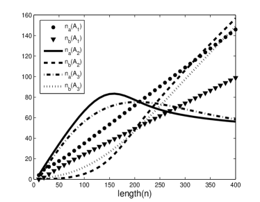
Figure 7:  Comparison of length dependence under three different assumptions. Case $A_{1}$ with $s=1.15$, $\sigma=0.037$, $w=1.03$, $p=0.072$ and $\eta=1$. Case $A_{2}$ with $s=1.14$, $\sigma=0.04$, $w=1.07$, $p=0.0062$ and $\eta=1$. Case $A_{3}$ with $s=1.14$, $\sigma=0.0047$, $w=1.03$, $p=0.007$ and $\eta=1$. The values of parameters in case $A_{1}$ are the same as in Fig. 4. The values of parameters in case $A_{2}$ and $A_{3}$ are chosen to best fit the PDB data between $n=10-200$ .

References

- (1) Branden, C., Tooze, J., Introduction to protein structure. Garland Pub (1998).
- (2) Flory, P. J., Statistical mechanics of chain molecules. Hanser Pub (1988).
- (3) S.B.Prusiner, Molecular biology of prion diseases, Science. 252, 1515-1522 (1991).
- (4) Patel, S., Balaji, P. V., Sasidhar, Y. U., The sequence TGAAKAVALVL from glyceraldehyde-3-phosphate dehydrogenase displays structural ambivalence and interconverts between -helical and -hairpin conformations mediated by collapsed conformational states. J. Pept. Sci. 13, 314-326 (2007).
- (5) B.H. Zimm and J.K. Bragg, Theory of the phase transition between Helix and Random Coil in polypeptide chains, J. Chem. Phys., 31(1959), 526-535.
- (6) T.M. Birstein and O.B. Ptitsyn, Conformations of macromolecules. Interscience (1966).
- (7) C.W. David and R. Schor, Statistical-mechanical model for the transformation in keratins, J. Chem. Phys., 42, 2156-2157 (1965).
- (8) C.W. David, H.B. Haukaas, J.G. Kalnins and R. Schor, Statistical-mechanical study of the transformation in keratins II. The tension-length isotherms, Biophysical Journal, 7, 505-510 (1967).
- (9) R. Schor, H.B. Haukaas and C.W. David, Statistical-mechanical studies of the transformation in keratins III. A monte-carlo simulation, J. Chem. Phys., 49, 4726-4727 (1968).
- (10) A.V. Finkelstein, Predicted -structure stability parameters under experimental test, Protein Engineering 8, 207-209 (1995).
- (11) C.A.Rohl and A.J.Doig, Models for the -helix/coil,-helix/coil, and -helix/-helix/coil transitions in isolated peptides, Protein Science. 5, 1687-1696 (1996).
- (12) H.Qian and J.A.Schellman, Helix-coil theories: a comparative study for finite length polypeptides, J.Phys.Chem. 96, 3987-3994 (1992).
- (13) D.Poland and H.A.Scheraga, Theory of helix-coil transitions in biopolymers. Academic Press (1970).
- (14) A.Y.Grosberg and A.R.Khokhlov, Statistical Physics of Macromolecules. AIP Press (1994).
- (15) S.Lifson and A.Roig, On the theory of helix-coil transition in polypeptides, J. Chem. Phys., 34, 1963-1974 (1961).