Fick’s law and Fokker-Planck Equation in inhomogeneous environments

Abstract

In inhomogeneous environments, the correct expression of the diffusive flux is not always given by the Fick’s law $\Gamma=-D\nabla n$. The most general hydrodynamic equation modelling diffusion is indeed the Fokker-Planck Equation (FPE). The microscopic dynamics of each specific system may affect the form of the FPE, either establishing connections between the diffusion and the convection term, as well as providing supplementary terms. In particular, the Fick’s form for the Diffusion Equation may arise only in consequence of a specific kind of microscopic dynamics. It is also shown how, in the presence of sharp inhomogeneities, even the hydrodynamic FPE limit may becomes inaccurate and mask some features of the true solution, as computed from the Master Equation.

Introduction. The fluid modelling of the time- and space evolution of quantities within complex environments, whose dynamics may only be treated on statistical grounds, is made using the diffusion equation (DE) $\partial_{t}n=D\partial_{x}^{2}n$. This phenomenological equation arises from two more fundamental equations: the continuity equation for $n$: $\partial_{t}n=-\partial_{x}\Gamma$, and the Fick’s law (or Fourier’s law) ref1 $\Gamma=-D\partial_{x}n$, where $x$ and $t$ are the spatial coordinate and the time, respectively; the diffusivity $D$ is a constant dependent from the medium. A pedagogical overview of Fick’s (Fourier’s) law and diffusion equation may be found in ghosh .
The postulate of homogeneity may hold just as a first-order approximation, whereas most systems must ultimately allow for some degree of non-uniformity. Almost unavoidably, therefore, one is faced with the question: how DE has to be generalized to such systems. The exact answer to this question is of relevance for a plethora of problems in practically any branch of natural sciences: from physics, to chemistry, geology, biology, social sciences, ….
Heuristically, the difficulty related to the generalization of DE may be understood as follows: an inhomogeneous environment should make $D$ position-dependent: $D\to D(x)$. There are, however, several choices for $\Gamma{}$ that differ when $D=D(x)$, but that collapse to the same identical form when $D$ is constant. Therefore, the problem may be restated as: what is the correct generalization of Fick’s law (provided that one exists) in inhomogeneous environments.
This subject appears repeatedly addressed in literature; however, it is difficult to find the explicit exposition of a general solution. In Van Kampen’s book ref2 , it is argued that one cannot decide a priori what the correct form for $\Gamma{}$ is, which rather depends upon the properties of the problem studied. Landsberg (ref3 and references therein), points out that, to some extent, it is a matter of convention, provided that supplementary (convective) terms are added suitably. In other terms, the definition of a diffusive and a convective flux is not univocal, only the total flux is. The paper providing the clearest intuitive insight and at the same time detailed calculations about what goes on in such situations is probably Schnitzer’s ref4 . We mention also the papers ref5 ; ref5bis , featuring computer experiments and presenting further bibliography about this subject. Papers ref5ter ; ref6 ; ref7 feature analytical and experimental work, demonstrating that the straightforward generalization of Fick’s law $\Gamma=-D(x)\partial_{x}n(x)$ cannot hold in all systems.

In order to quantitatively address the issue, it is necessary to deal with a reasonably accurate modelling of the dynamics at the microscopic level: transport equations, thus, will emerge at the level of large length scales. The tool we adopt is provided by the Master Equation (ME):

$$\frac{{\partial n(x,t)}}{{\partial t}}=-\frac{{n(x,t)}}{{\tau(x)}}+\int{dx^{\prime}p(x-x^{\prime},x^{\prime})\frac{{n(x^{\prime},t)}}{{\tau(x^{\prime})}}}$$ (1)

ME (1) yields a coarse grained probabilistic description of a microscopic system driven by a Markov process, and can be visualized as the continuity equation for the passive scalar quantity n(x,t) (which, properly speaking, is a probability density) subject to transitions (“jumps”) modifying its state from $x^{\prime}$ to $x$, with probability $p(x-x^{\prime},x^{\prime})$, and at a rate $1/\tau{}(x)$ (see chapter 1 of langevin ). Equation (1) contains virtually all the solutions of the transport problem, once the functions $p$ and $\tau{}$ are given. On the other hand, it is often unpractical to deal directly with it, particularly in higher-dimensional problems. Therefore, and particularly if a clear-cut separation of scales exists in the problem studied, it is customary to take its long-wavelength limit, which washes out details at the finest scales and turns the integral equation (1) into a famous differential equation: the Fokker-Planck Equation (FPE) (see, e.g., chapter 9 of balescu ):

$$\frac{{\partial n(x,t)}}{{\partial t}}=-\frac{\partial}{{\partial x}}\left({U(x)n}\right)+\frac{{\partial^{2}}}{{\partial x^{2}}}\left({D(x)n}\right)$$ (2)

Within the ME formulation, all the physics is built into the functions $p$ and $\tau$. In the passage from ME to FPE, $p$ and $\tau$ are packed into the diffusive and convective terms, $D,U$. Therefore, the analytical expression of $D,U$, ultimately relies on the constraints that the problem to be solved places on $p,\tau$. Is it possible, basing upon general considerations on the microscopic dynamics, to identify equivalent classes of systems, that is, systems that lead to the same qualitative form of the FPE ? As we shall show later, the initial question advanced in this Introduction is related to this point: the Fick’s form of the diffusion equation is a particular limiting case of the FPE, that arises when the microscopic dynamics fulfils a given simmetry.
The purpose of this paper is to provide a discussion about this topic. Furthermore, we will address the broader issue of the validity of the scale separation at the basis of the FPE. We will show that, whenever, this hypothesis is not fulfilled, additional terms to the FPE need to be considered.
From the Master Equation to the Fokker-Planck Equation. The simplest way to pass from ME to FPE is by expressing the integrand in Eq. (1) in terms of the small parameter $\Delta{}=x^{\prime}-x$, which is of order the mean jumping length $L_{p}$:

$${p(x-x^{\prime},x^{\prime})\over\tau(x^{\prime})}n(x^{\prime})={p(-\Delta,x+\Delta)\over\tau(x+\Delta)}n(x+\Delta)$$ (3)

and expanding around $x$ in powers of $\Delta$ (Kramer-Moyal expansion). However, this step is justified provided that $p,\tau,n$, are not strongly varying functions of $x$ over distances of order $L_{p}$. If we assume that $n$ is a smooth function of $x$, we may concentrate on the other quantity: $h=p/\tau$. A branching into two cases is possible: (1) $h$ is a smooth function, or (2) $h$ is not. Although, condition (2) actually contains (1) as a particular case, it turns out convenient to consider them separately, since (1) is easier to deal with.
Finally, we will consider also the case (3), when $n$ itself is not a smooth function.
Case (1): both $n$ and $h$ are smooth functions. We are allowed to make a Taylor expansion in powers of the function $h\times n$. The result, truncated to second order, yields Eq. (2) with

$$U=\int{d\Delta\frac{{p(\Delta,x)}}{{\tau(x)}}}\Delta\,,\quad D={1\over 2}\int{d\Delta\frac{{p(\Delta,x)}}{{\tau(x)}}}\Delta^{2}$$ (4)

Limiting the truncation to second order is ordinarily justified on the basis of Pawula theorem ref8 ; ref9 .
All the information relevant to our problem is packed into $U,D$. Two important cases are (A) $U=(dD/dx)$, or (B) $U=0$. Case (A) recovers Fick’s law, while case (B) yields the solution

$$\partial_{t}n=\partial^{2}_{x}(D(x)n(x))$$ (5)

Both results may be verified by direct substitution into Eq. (2). It turns out that relation (A) arises straightforwardly from ME (1) by postulating the simmetry

$$\frac{{p(x^{\prime}-x,x)}}{{\tau(x)}}=\frac{{p(x-x^{\prime},x^{\prime})}}{{\tau(x^{\prime})}}\to\frac{{p(\Delta,x)}}{{\tau(x)}}=\frac{{p(-\Delta,x+\Delta)}}{{\tau(x+\Delta)}}$$ (6)

which ensures the time reversal symmetry of the microscopic dynamics. Indeed, a first-order Taylor expansion of the second argument around $x$ yields, after rearranging,

$$\Delta\frac{{dp(-\Delta,x)}}{{dx}}=p(\Delta,x)-p(-\Delta,x)+\Delta{\kern 1.0pt}p(-\Delta,x)\frac{{d\ln\tau}}{{dx}}$$ (7)

Using Eq. (7) into the integrals (4) yields the sought result (A) (For a different derivation, see Prof. Feder’s lecture notes federURL ).
The solution (B) has some relevance, too, since it corresponds to the choice of a symmetrical kernel: $p(\Delta,x)=p(-\Delta,x)$. Although apparently natural, the range of validity of this condition is actually rather narrow, as it cannot hold under smoothly varying conditions, where $p(\Delta,x)\neq p(-\Delta,x)$; that is, the probability for a particle of jumping rightwards or leftwards cannot be the same. In order to better understand this point, let us consider a system where test particles collide against some scattering centres. Jumps are arcs of ballistic motion between two collisions. If the system is not homogeneous the density $n_{sc}$ of the scattering centres is not uniform. Let us suppose, say, $dn_{sc}/dx<0$: a test particle at $x$ has a larger probability of striking a scattering centre that is on its left ($x-\delta x$) rather than on its right ($x+\delta x$), and therefore of being backscattered in the opposite direction. Hence, there is a larger probability of bouncing back rightwards than the converse.
Having ruled out the case (B) for several inhomogeneous systems, one could wonder how general is condition (A). It turns out that (A) generically holds for a large class of 1-degree-of-freedom Hamiltonian systems ref10 ; ref11 ; ref12 (see also feder1 for another particular case). For more general systems, and especially in systems with more degrees of freedom, the above constraints between $U$ and $D$ cannot be guaranteed to hold any longer, and FPE may allow in principle for a wide variety of cases. Two such instances, recalled in ref10 , are: the self-consistent motion of charged particles in a set of Langmuir waves, and the 2-dimensional guiding-centre motion of a particle in a varying stochastic electrostatic field.
Case (2): $n$ is a smooth function but $h$ is not. Let us consider case (2), when $p$ and/or $\tau$ present sharp variations: we mean they vary on scales smaller than $L_{p}$. This is the situation when one needs modelling systems characterized by sudden transitions between regions with widely different physical properties. Therefore one is forced to study the case when we can still expand $n$ in powers, but now must leave $h$ unexpanded: after some calculations

$${\partial n\over\partial t}={\partial^{2}\over\partial x^{2}}\left(\hat{D}n\right)-{\partial\over\partial x}\left(\hat{U}n\right)+\hat{W}n$$ (8)

$$\hat{D} = {\hat{m}_{2}\over 2}$$

$$\hat{U} = \hat{m}_{1}+\partial_{x}\hat{m}_{2}$$

$$\hat{W} = {\partial_{x}^{2}\hat{m}_{2}\over 2}+\partial_{x}\hat{m}_{1}+\hat{m}_{0}$$

$$\hat{m}_{j} = \int{dx^{\prime}(x-x^{\prime})^{j}\frac{{p(x-x^{\prime},x^{\prime})}}{{\tau(x^{\prime})}}}-\delta_{j0}\frac{1}{{\tau(x)}}\;\;(j=0,1,2)$$

We have now an “extended” Fokker-Planck Equation, due to the presence of an additional $\hat{W}n$ term. One may feel unconfortable about the presence of this term, since at first sight it appears to spoil the conservation of matter: $\partial N/\partial t=\partial\int n/\partial t=0$, which is built into Eq. (1) and Eq. (2). By integrating Eq. (8) over $x$, instead, one has $\partial N/\partial t=\int\hat{W}n(x)dx$, which is not granted a priori to be zero. We will show, instead, that it is exactly the case: the role of $\hat{W}$ is that of transferring matter from one point to another, rather than that of a net sink or source. Heuristically, it may be guessed on the basis of the fact that Eq. (8) is just an intermediate passage in the chain of calculations leading from Eq. (1) to Eq. (2). Since both the starting and the end expressions do conserve matter, also the intermediate step must. For simplicity, from here on, we will consider the case of constant $\tau=1$; hence, only variations in $p$ will be dealt with. Let $x_{0}$ be a point around which $p$ shows a sharp variation. For the sake of simplicity, let us consider a step-like variation around $x_{0}=0$:

$$p(x-x^{\prime},x^{\prime})=\left\{\begin{array}[]{*{16}c}{p_{L}(x-x^{\prime})\quad x^{\prime}<0}\\ {p_{R}(x-x^{\prime})\quad x^{\prime}>0}\\ \end{array}\right.$$ (9)

Since, far from $x_{0}$, the system is almost homogeneous, we may suppose that the jumping lengths are symmetrical: $p_{L,R}(x-x^{\prime})=p_{L,R}(|x-x^{\prime}|)$. We show now that, under these hypotheses, $\hat{W}$ reverses sign around $x_{0}=0$: $\hat{W}(-x)=-\hat{W}(x)$. For brevity, we proceed to demonstrate only that $\hat{m}_{0}$ is an odd function of $x$. Calculations for the other two terms carry on along the same lines:

$$\hat{m}_{0}(x) = \int dx^{\prime}p(x-x^{\prime},x^{\prime})-1=\int_{x^{\prime}<0}dx^{\prime}p_{L}(x-x^{\prime})+\int_{x^{\prime}>0}dx^{\prime}p_{R}(x-x^{\prime})-1$$ (10)

$$= \int dx^{\prime}p_{L}(x-x^{\prime})+\int dx^{\prime}p_{R}(x-x^{\prime})-\int_{x^{\prime}>0}dx^{\prime}p_{L}(x-x^{\prime})-\int_{x^{\prime}<0}dx^{\prime}p_{R}(x-x^{\prime})-1$$

$$= 1+1-\int_{x^{\prime}>0}dx^{\prime}p_{L}(x-x^{\prime})-\int_{x^{\prime}<0}dx^{\prime}p_{R}(x-x^{\prime})-1$$

$$= -\left(\int_{x^{\prime}>0}dx^{\prime}p_{L}(x-x^{\prime})+\int_{x^{\prime}<0}dx^{\prime}p_{R}(x-x^{\prime})-1\right)$$

If in the last line we make the change of variables $x\to-x,x^{\prime}\to-x^{\prime}$, we get that the term within parentheses is just $\hat{m}_{0}(-x)$. The second fundamental property of $\hat{W}$ is that $\hat{W}$ is different from zero only over a region around $x=0$ of width a few jumping lengths: It is straightforward to show that $\hat{m}_{0}=d\hat{m}_{1}/dx=d^{2}\hat{m}_{2}/dx^{2}=0$ when $|x|>>L_{p}$ . On the other hand, $n$ is just a weakly varying function over distances of order the jumping length: this is a postulate implicit in the Taylor expansion done when going from Eq. (1) to Eq. (8). Therefore, combining the above results, $\int\hat{W}(x)n(x)\;dx\approx n(0)\int\hat{W}(x)\;dx$, and $\int\hat{W}\;dx=0$. This concludes the demonstration.
In order to be more quantitative, let us consider the paradigmatic case of a gaussian diffusion with sharp variations of the jumping length:

$$p(x-x^{\prime},x^{\prime}) = \frac{1}{{\sqrt{2\pi\sigma^{2}(x^{\prime})}}}\exp\left[{-\frac{{(x-x^{\prime})^{2}}}{{2\sigma^{2}(x^{\prime})}}}\right]$$ (11)

$$\sigma(x) = \left\{{\begin{array}[]{*{16}c}{\sigma_{L}\;\;,\quad x<0}\\ {\sigma_{R}\;\;,\quad x>0}\\ \end{array}}\right.$$ (14)

It is straightforward to compute $\hat{W}$ for this system:

$$\hat{W} = \sqrt{\frac{1}{8\pi}}x\left(\frac{e^{-\frac{x^{2}}{2\sigma_{R}^{2}}}\left(4\sigma_{R}^{2}-x^{2}\right)}{\sigma_{R}^{3}}+\frac{e^{-\frac{x^{2}}{2\sigma_{L}^{2}}}\left(x^{2}-4\sigma_{L}^{2}\right)}{\sigma_{L}^{3}}\right)$$ (15)

$$- \frac{1}{2}\left(\text{erf}\left(\frac{x}{\sqrt{2}\sigma_{L}}\right)-\text{erf}\left(\frac{x}{\sqrt{2}\sigma_{R}}\right)\right)$$

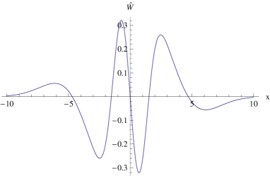
Figure 1: $\hat{W}$ from Eq. (15), with $\sigma_{L}=1$, $\sigma_{R}=2.5$.

Its profile is given in figure (1).
We have available an excellent experimental test bench of this result: paper ref7 presents a study of tracer diffusion between gelatine solutions with different viscosity, which means different effective diffusivity. The width of the interface between the two solution is very small, and can be considered as zero for our purposes. Hence, the whole system may be modelled as two regions with different jumping lengths, just done above. It is apparent at this point that applying Eq. (2) at this problem is of dubious validity, since $p$ is discontinuous at $x^{\prime}=0$ in its second argument. Nevertheless, just as an exercise, we may formally evaluate $U,D$, for this choice of $p$:

$$U=0\,,\quad D={1\over 2}\left\{{\begin{array}[]{*{20}c}{\sigma_{L}^{2}\;,\quad x<0}\\ {\sigma_{R}^{2}\;,\quad x>0}\\ \end{array}}\right.$$ (16)

thereby recovering Eq. (5). $\hat{W}$ appearing in (8) has been computed in Eq. (15), and $\hat{D},\hat{U}$ are analytically computable alike, although we do not provide their complete expression here for saving space. The numerical values we choose for $\sigma_{L,R}$ are $\sigma_{L}=\sqrt{2.4}$, $\sigma_{R}=\sqrt{5.8}$, and solve for the time evolution of $n(x,t)$ starting from a flat profile: $n(x,t=0)=1$. In Fig. (2) we show the spatial profile at a later time for the solution of Eq. (8) as well as of Eq. (5). These profiles should be compared against their counterpart from experiments (Fig. 5 in ref. ref7 ). It becomes apparent that the smooth transition around $x=0$, that exists in real data, is completely masked by the use of Eq. (5), while is correctly recovered by Eq. (8).

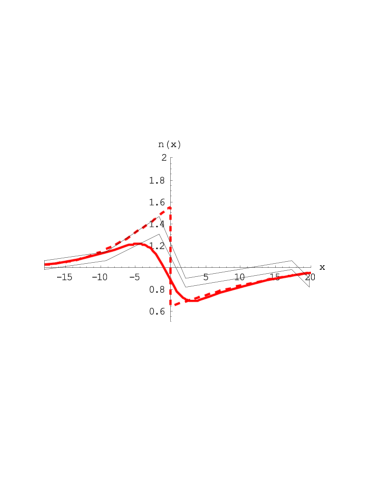
Figure 2: (Color online) Solution of Eq. (8) (solid line) and Eq. (5) (dashed line) at $t=32$. Starting profile is flat: $n(t=0)=1$. The contoured region roughly envelops the area where experimental points lie (adapted from Fig. 5 of Ref. ref7 ). The two solutions are computed for slightly different boundary conditions: Eq. (8) has been numerically solved imposing $dn/dx=0$ at $x=\pm 40$. Eq. (5) may be integrated analytically. Its solution is discontinuous in $x=0$, but the flux $d(Dn)/dx$ is continuous ref7 . For this function, $dn/dx\to 0$ only asymptotically as $|{}x|{}\to\infty{}$.

Case (3): $n$ is not a smooth function and the full Master Equation is needed. This case acquires relevance when variations in $n$ occur over scales smaller than the jumping length: $L_{p}>L_{n}\equiv{}n/(dn/dx)$. In unbounded not driven systems this criterion may be satisfied only transiently, starting from highly localized profiles. Left to itself, density relaxes so as to fulfil $L_{n}>L_{p}$. However, $L_{n}$ may be bounded by imposing absorbing boundaries. Hence, $L_{n}<L$, where $L$ is the system’ size. Since absorbing boundaries imply loss of density from the system, in order to maintain a steady state it is necessary to add a source, which is parameterized by its spatial extension, and hence a further typical length, $L_{s}$. The usual ordering is $L_{p}<L_{s}<L$, while now we investigate the reversal of this ordering. For simplicity, we will limit to consider the steady state $\partial{\kern 1.0pt}/\partial t=0$. Eq. (1) with a source $S$ can be solved in Fourier space for $g(x)=n(x)/\tau{}(x)$:

$$g(k)=\frac{{S(kL_{s})}}{{1-p(kL_{p})}}$$ (17)

In (17) we have made it explicit that $p$ depends upon scale length $L_{p}$, and $S$ upon $L_{s}$. For $kL_{p},kL_{s}<<1$, one recovers the solution of the diffusion equation if $p$ is a smooth symmetrical function: $1-p(k)\approx k^{2},\,k\to 0$. (If $p$ lacks mirror symmetry, a convective term appears). Hence, over very large spatial scales one does not expect any novel feature to arise. However, when $kL_{s}\approx 1$ but $kL_{p}>>1$ the denominator of (17) is almost one: $p$ must have finite support, thus $p\to 0,k\to\infty$. Hence

$$g(k)\approx S(k)$$ (18)

Close to the source, and over distances of order of the source’s width, the density profile matches exactly that of $S$. This is an effect totally unpredictable within the FPE formulation, that instead would smear the density throughout the whole system. In order to check numerically this prediction, we have solved Eq. (1) for a given source profile and different values of $L_{p}$. The results, fully confirming our analytical estimates, are shown in Fig. (3).

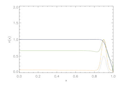
Figure 3: (Color online) Density profiles $n$ due to the source (dashed curve) for three values of $L_{p}=0.0125$ (black curve), 0.125 (green curve), 1 (orange curve). Here, the container has size $L=1$, and the source width is $L_{s}=0.025$. Reflecting conditions are imposed at $x=0$ and absorbing boundaries at $x=1$.

Conclusions. In summary, inhomogeneity may have dramatic effect on the modelling of the spreading of some quantity into a medium. It affects the writing of the equation of motion, turning it into a problem that has unambiguous solutions, but generally not valid ones for all classes of systems. Two fundamental criteria are identified. From the one hand, the microscopic dynamics imposes constraints between the diffusive and convective coefficients of the FPE. On the other hand, the form of the FPE itself depends on the existence of scale separation between typical lengths existing in the system: when this criterion is fulfilled and transport scales are clearly smaller than any other scale, the classical FPE is valid. On the opposite side, when no clear separation can be made, additional terms need to be added into an “augmented” FPE, till to the extreme case, where only the full ME may provide correct results. The first criterion is obviously the most important: FPE is often used for modelling purposes starting from a limited knowledge of the underlying microscopic dynamics. Clearly, one cannot establish a priori if scale separation does hold in the problem at hand. In these situations, therefore, the standard FPE has to be used, the only risk being that of missing some small-scale features.

Acknowledgements. Interactions with G. Spizzo, S. Cappello, and D.F. Escande are acknowledged. L. Salasnich, G. Serianni and Prof. J. Feder provided useful references. The referees made unvaluable comments in order to improve the manuscript. This work was supported by the European Communities under the Contract of Association between Euratom/ENEA.

References

- (1) A. Fick, Phil. Mag. 10, 30 (1855)
- (2) K. Ghosh, et al, Am. J. Phys. 74, 123 (2006)
- (3) N.G. Van Kampen, Stochastic Processes in Physics and Chemistry (North-Holland, 1981), ch. 10.3
- (4) P.T. Landsberg, J. Appl. Phys. 56, 1119 (1984)
- (5) M.J. Schnitzer, Phys. Rev. E 48, 2553 (1993)
- (6) R. Collins, S.R. Carson, and J.A.D. Matthew, Am. J. Phys. 63, 230 (1997)
- (7) L. Tao, M.R.E. Proctor, N.O. Weiss, Mon. Not. R. Astron. Soc. 300, 907 (1998)
- (8) N.H. Bian, O.E. Garcia, Phys. Plasmas 12, 042307 (2005)
- (9) P. Lançon, G. Batrouni, L. Lobry, and N. Ostrovsky, Europhys. Lett. 54, 28 (2001)
- (10) B.Ph. Van Milligen, P.D. Bons, B.A. Carreras, and R. Sánchez, Eur. J. Phys. 26, 913 (2005)
- (11) W.T. Coffey, Yu P. Kalmykov and J.T. Waldron, The Langevin Equation (World Scientific, 1996)
- (12) R. Balescu, Statistical Dynamics (Imperial College Press, 1997)
- (13) H. Risken, The Fokker-Planck Equation: Methods of Solutions and Applications (Springer, 1989)
- (14) R.F. Pawula, Phys. Rev. 162, 186 (1967)
- (15) http://folk.uio.no/feder/Fys3130/LectureNotes/FokkerPlanck.pdf
- (16) D.F. Escande and F. Sattin, Phys. Rev. Lett. 99, 185005 (2007)
- (17) A.J. Lichtenberg, M.A. Lieberman, Regular and Stochastic Motion (Springer-Verlag, 1983)
- (18) Y. Elskens and D.F. Escande, Microscopic Dynamics of Plasmas and Chaos (Institute of Physics Publishing, 2003)
- (19) J. Feder, K.C. Russell, J. Lothe, and G.M. Pound, Adv. Phys. 15, 111 (1966)