Artificial viscosity in simulation of shock waves by smoothed particle hydrodynamics

Abstract

The artificial viscosity is reconsidered in smoothed particle hydrodynamics to prevent inter-particle penetration, unwanted heating, and unphysical solutions. The coefficients in the Monaghan’s standard artificial viscosity are considered as time variable, and a restriction on them is proposed such that avoiding the undesired effects in the subsonic regions. The shock formation in adiabatic and isothermal cases are used to study the ability of this modified artificial viscosity recipe. The computer experiments show that the proposal appears to work and the accuracy of this restriction is acceptable.

1 Introduction

Gas dynamical processes are believed to play an important role in the evolution of astrophysical systems on all length scales. A ubiquitous process in astrophysical fluid dynamics is the behavior of gases subjected by shock waves. These are almost the normal, rather than exceptional, type of astrophysical fluid flows that happen very often in cases of astrophysical interest. A number of examples are the onset of spiral structures and shock fronts in accretion disks around compact objects (Lanzafame et al. 2006), molecular cloud formation in shock-compressed layers (Koyama and Inutsuka 2000), the rapid and strong increase in pressure that can be produced by interaction of the fast wind and the slow envelope of a planetary nebulae (Gurzadyan 1997), and so on.

A powerful gridless particle method that was invented to solve complex fluid-dynamical problems in astrophysics is smoothed particle hydrodynamics (SPH) (Lucy 1977, Gingold and Monaghan 1977). The SPH method has a number of attractive features such as its low numerical diffusion in comparison to grid based methods. Whilst the SPH originally developed for compressible flows, it has been extended to deal with free-surface incompressible fluids (e.g., Monaghan 1994, Ellero et al. 2007). A recent worthy review of the SPH methodology and its applications can be found in Monaghan (2005).

An adequate scenario for SPH application is the unbound astrophysical problems, especially the behavior of gases subjected to compression (shock waves). The magnitude of the viscous term dose not affect the net shock-jump conditions, thus, many numerical schemes implicitly or explicitly incorporate the trick of artificial viscosity (AV) for halting the ever-growing steepening tendency produced by nonlinear effects. The first use of viscosity in SPH equations was by Lucy (1977) who introduced an AV to present a slow build-up of acoustic energy from integration errors in an SPH simulation. The AV is designed to allow shock phenomena to be simulated, or simply to stabilize a numerical algorithm. Indeed two forms of AV are applied in SPH equations, the bulk and the von Neumann-Richtmeyer viscosity, respectively. They prevent inter-particle penetration, allow shocks to form and damp the post-shock oscillations. Although many different functional forms for the AV have been proposed (see, e.g., Liu & Liu 2003), all contain problem sensitive parameters that are often set in a somewhat arbitrary manner. Here we try firstly to provide a guide to the relevant prescriptions for some AV that have been considered before.

A more effective viscosity which may conserves linear and angular momentum was suggested by Monaghan and Gingold (1983). They devised a viscosity by simple arguments about its form and its relation to gas viscosity. The viscous term between two particles, denoted by $\Pi_{ab}$, is added to the pressure term of SPH equations. When two particles approach each other, the AV produces a repulsive force between them. When they recede from each other the force is attractive (Monaghan 1989).

An undesirable aspect of the Monaghan’s standard AV is that it can introduce considerable shear viscosity into the flow. This problem may be reduced by a bulk viscosity in a general-purpose code of Hernquist and Katz (1989) for evolving three-dimensional, self-gravitating fluids in astrophysics. Clearly the artificial viscous dissipation increases the Reynolds number of a flow, artificially, with the result that, for example, the Kelvin-Helmholtz shear instabilities are heavily diffused. In this way a von Neumann stability analysis of the SPH equations along with a critical discussion of various parts of the algorithm was investigated by Balsara (1995). He suggested reducing viscous dissipation by multiplying $\Pi_{ab}$ by a symmetric factor.

Another problem of viscosity is that although AV is approximately successful for handling shocks but it can be too large in other parts of the flow. For this purpose, a switch to reduce the AV away from shocks was given by Morris and Monaghan (1997, hereafter MM97). They introduce the idea of time-varying switch which fits more naturally with a particle formulation. Each particle has a viscosity parameter which evolves according to a simple source and decay equation. The source causes the switch to grow when the particle enters a shock and the decay term causes it to decay to a small value beyond the shock.

In the present study we combine the Monaghan’s standard AV with the time-varying coefficients like that of MM97’s switch. we propose a modification to the time-dependent AV prescription designed by MM97 so that the aim is to maintain the shock-simulating capabilities of SPH. For this purpose we optimize the source term so that the AV is restricted to supersonic velocities in regions that are under compression. Section 2 is devoted to the SPH method and the suggested changes in the AV. These modifications have been tested in §3 for the one dimensional adiabatic and isothermal shock problems. Finally, a summary with conclusion is given in section 4.

2 The SPH methodology

The SPH was invented to simulate nonaxisymmetric phenomena in astrophysics (Lucy 1977, Gingold & Monaghan 1977). In this method, fluid is represented by $N$ discrete but extended/smoothed particles (i.e. Lagrangian sample points). The particles are overlapping, so that all the involved physical quantities can be treated as continuous functions both in space and time. Overlapping is represented by the kernel function, $W_{ab}\equiv W(\textbf{r}_{a}-\textbf{r}_{b},h_{ab})$, where $h_{ab}\equiv(h_{a}+h_{b})/2$ is the mean smoothing length of two particles $a$ and $b$. The continuum equations are (Monaghan 1992)

$$\rho_{a}=\sum_{b}m_{b}W_{ab}$$ (1)

$$\frac{d\textbf{v}_{a}}{dt}=-\sum_{b}m_{b}(\frac{p_{a}}{\rho_{a}^{2}}+\frac{p_{b}}{\rho_{b}^{2}}+\Pi_{ab})\nabla_{a}W_{ab}$$ (2)

$$\frac{du_{a}}{dt}=\frac{1}{2}\sum_{b}m_{b}(\frac{p_{a}}{\rho_{a}^{2}}+\frac{p_{b}}{\rho_{b}^{2}}+\Pi_{ab})\textbf{v}_{ab}\cdot\nabla_{a}W_{ab}$$ (3)

where $\textbf{v}_{ab}\equiv\textbf{v}_{a}-\textbf{v}_{b}$, the AV between particles $a$ and $b$ is presented by $\Pi_{ab}$, and the other notations have their usual meanings.

2.1 Viscosity

In order to simulate the shock problems of hydrodynamics, special treatments or methods are required to allow the algorithms to be capable of modeling shock waves, or else the simulation will develop unphysical oscillations in the numerical results around the shocked regions. A shock wave is not a true physical discontinuity, but a very narrow transition zone whose thickness is usually in the order of a few molecular mean free paths. Application of the conservation of mass, momentum, and energy conditions across a shock front requires the simulation of transformation of kinetic energy into heat energy. Physically this energy transformation can be represented as a form of viscous dissipation. This idea leads to the development of the von Neumann-Richtmyer AV that is needed only to be present during material compression,

$$\Pi_{1}=\cases{a_{1}(\triangle x)^{2}\rho(\nabla.\mathbf{v})^{2}&$\nabla.\mathbf{v}<0$\cr 0&$\nabla.\mathbf{v}\geq 0$,}$$ (4)

where $a_{1}$ is an adjustable non-dimensional constant. It is found that adding the following linear AV term,

$$\Pi_{2}=\cases{a_{2}(\triangle x)c\rho(\nabla.\mathbf{v})&$\nabla.\mathbf{v}<0$\cr 0&$\nabla.\mathbf{v}\geq 0$,}$$ (5)

where $c$ is the sound speed and $a_{2}$ is another non-dimensional constant (Liu and Liu 2003), has the advantage of further smoothing the oscillations that are not totally dampened by the quadratic AV term, equation (4).

The most widely used AV in SPH is that of Monaghan (1989), which not only provides the necessary dissipation to convert kinetic energy into heat at the shock front, but also prevent unphysical penetration for particles approaching each other. The detailed formulation is as follows:

$$\Pi_{ab}=\cases{\frac{-\alpha v_{sig}\mu_{ab}+\beta\mu_{ab}^{2}}{\bar{\rho}_{ab}},&if $\textbf{v}_{ab}.\textbf{r}_{ab}<0$,\cr 0,&otherwise,}$$ (6)

where $\bar{\rho}_{ab}=\frac{1}{2}(\rho_{a}+\rho_{b})$ is an average density, $\alpha\sim 1$ and $\beta\sim 2$ are the artificial coefficients, and $\mu_{ab}$ is defined as its usual form

$$\mu_{ab}=\frac{\textbf{v}_{ab}\cdot\textbf{r}_{ab}}{\bar{h}_{ab}}\frac{1}{r_{ab}^{2}/\bar{h}_{ab}^{2}+\eta^{2}}$$ (7)

with $\eta\sim 0.1$ and $\bar{h}_{ab}=\frac{1}{2}(h_{a}+h_{b})$. The signal velocity, $v_{sig}$, is

$$v_{sig}=\frac{1}{2}(c_{a}+c_{b})$$ (8)

where $c_{a}$ and $c_{b}$ are the sound speed of particles.

Since the Monaghan type AV introduces a shear viscosity into the flows especially in regions away from the shock, an AV depending on the divergence of the velocity field was employed by Hernquist and Katz (1989),

$$\Pi_{ab}=\frac{q_{a}}{\rho_{a}^{2}}+\frac{q_{b}}{\rho_{b}^{2}},$$ (9)

where

$$q_{a}=\cases{\alpha h_{a}\rho_{a}c_{a}|\nabla.\mathbf{v}|_{a}+\beta h_{a}^{2}\rho_{a}|\nabla.\mathbf{v}|_{a}^{2}&$\nabla.\mathbf{v}<0$\cr 0&otherwise.}$$ (10)

This AV can lead to spurious results if particles $a$ and $b$ are receding; i.e., such terms will contribute viscous artificial cooling. To avoid this problem, Hernquist and Katz (1989) set $\Pi_{ab}=0$ if $\mathbf{v}_{ab}.\mathbf{r}_{ab}>0$; a decision which may, in some cases, add small amounts of shear viscosity. In this approach, determining $\Pi_{ab}$ by referring to binary interaction, effectively, gives an idea about the molecular bulk fluid descriptions.

Other view on the Monaghan’s standard AV was also proposed by Balsara (1995) who developed a modification of the AV term that approximately sets the dissipation to zero in regions of pure shear, while leaving it unaffected in regions of compression. This is done by suggestion

$$\Pi_{ab}=\left(\frac{p_{a}}{\rho_{a}^{2}}+\frac{p_{b}}{\rho_{b}^{2}}\right)(-\alpha\mu_{ab}+\beta\mu_{ab}^{2}),$$ (11)

where a switch in the form of a multiplicative factor ($\mu_{ab}\rightarrow\mu_{ab}f_{ab}/\bar{c}_{ab}$) was introduced. The factor $f_{ab}$ is the average of $f_{a}$ and $f_{b}$, where

$$f_{a}=\frac{|\nabla.\mathbf{v}|_{a}}{|\nabla.\mathbf{v}|_{a}+|\nabla\times\mathbf{v}|_{a}+10^{-4}c_{a}/h_{a}}.$$ (12)

The function $f_{a}$ acts as a switch, approaching unity in regions of compression ($|\nabla.\mathbf{v}|_{a}>>|\nabla\times\mathbf{v}|_{a}$) and vanishing in regions of large vorticity ($|\nabla\times\mathbf{v}|_{a}>>|\nabla.\mathbf{v}|_{a}$). Consequently, this AV has the advantage that it is suppressed in shear layers.

Meanwhile, MM97 carried the process further by introducing the idea of time-varying coefficients which fits more naturally with a particle formulation. In this method, the AV is given by

$$\Pi_{ab}=-\frac{K_{ab}v_{sig}\mathbf{v}_{ab}\cdot\mathbf{r}_{ab}}{\bar{\rho}_{ab}|\mathbf{r}_{ab}|},$$ (13)

where $K_{ab}=(K_{a}+K_{b})/2$ is a variable switch which should change with time according to the conditions the particle is in, becoming large at shocks, but relaxing back to a small value when the flow is calmer. Each particle $a$ has a viscosity switch which evolves according to a simple source,

$$\mathcal{S}_{a}=\max(-\nabla\cdot\mathbf{v}_{a},0),$$ (14)

and decay equation,

$$\frac{dK_{a}}{dt}=-\frac{K_{a}-K_{\mathrm{min}}}{\tau_{a}}+\mathcal{S}_{a},$$ (15)

such that in the absence of source term $\mathcal{S}_{a}$, the switch $K_{a}$ decays to a value $K_{\mathrm{min}}$ over a time scale $\tau_{a}\equiv h_{a}/(\mathcal{C}v_{sig})$. The dimensionless parameter $\mathcal{C}$ has a value $0.1<\mathcal{C}<0.2$. The source causes the switch to grow when the particle enters a shock and the decay term causes it to decay to a small value beyond the shock.

2.2 Restricted AV

In SPH the formation of shocks is mostly an effect of the von Neumann-Richtmeyer viscosity. To avoid the undesirable effects in the subsonic region, we propose to restrict the use of it to those regions. This modification will allow shocks to form, and prevent inter-particle penetration at supersonic velocities. When the gas has reached equilibrium, the pressure force prevents further compression. This process is not possible with source term (14) because of supersonic relative velocities of the particles at different regions of the shock. The AV as outlined by equation (13) will decelerate and heat the gas, and prevent enough compression. To weaken this problem, we use the following lemma.

Since $\rho_{a}\propto h_{a}^{-\nu}$ where $\nu$ is the dimension of the problem, the time derivative for any particle can be written as

$$\dot{\rho_{a}}=-\frac{\nu\rho_{a}\dot{h}_{a}}{h_{a}}.$$ (16)

This relation can be used to decide whether a particle follows the fluid or if the source term of AV is necessary. If two particles are approaching each other at velocity exceeding the signal velocity, that is if

$$r_{ab}(\frac{\dot{\rho}_{a}}{\rho_{a}}-\frac{\nu\dot{h}_{a}}{h_{a}})>v_{\mathrm{sig}},$$ (17)

AV is necessary to prevent inter-particle penetration. We therefore propose to restrict the source term of AV with defined frequency as

$$\omega_{a}\equiv\frac{\dot{\rho}_{a}}{\rho_{a}}-\frac{\nu\dot{h}_{a}}{h_{a}}-\frac{v_{\mathrm{sig}}}{r_{ab}}.$$ (18)

A good way to do this for a particle is to use the restricted source term $\mathcal{S}_{a}$, instead of equation (14), as follows

$$\mathcal{S}_{a}=\max(-\nabla.\mathbf{v}_{a},\omega_{a},0).$$ (19)

Base on a method similar MM97, we use $\alpha$ and $\beta$ in the standard AV, equation (6), in form of variables with respect to time,

$$\frac{d\alpha_{a}}{dt}=-\frac{\alpha_{a}-\alpha_{\mathrm{min}}}{\tau_{a}}+z_{\alpha}\mathcal{S}_{a},$$ (20)

and

$$\frac{d\beta_{a}}{dt}=-\frac{\beta_{a}-\beta_{\mathrm{min}}}{\tau_{a}}+z_{\beta}\mathcal{S}_{a},$$ (21)

respectively, where the parameters $z_{\alpha}$ and $z_{\beta}$ are chosen to regulate the effect of source term such that the heat production and post-shock oscillations are controlled in the numerical simulations.

3 Shock formation test

3.1 Analytical formulation

As outlined before, an extremely important problem is the behavior of gases subjected to compression waves. This happens very often in the cases of astrophysical interests. For example, a small region of gas suddenly heated by the liberation of energy will expand into its surroundings. The surroundings will be pushed and compressed, thus, a shock front is formed. Conservation of mass, momentum, and energy across a shock front is given by the Rankine-Hugoniot conditions (Dyson and Williams 1997)

$$\rho_{1}v_{1}=\rho_{2}v_{2}$$ (22)

$$\rho_{1}v_{1}^{2}+K\rho_{1}^{\gamma}=\rho_{2}v_{2}^{2}+K\rho_{2}^{\gamma}$$ (23)

$$\frac{1}{2}v_{1}^{2}+\frac{\gamma}{\gamma-1}K\rho_{1}^{\gamma-1}=\frac{1}{2}v_{2}^{2}+\frac{\gamma}{\gamma-1}K\rho_{2}^{\gamma-1}+Q$$ (24)

where the equation of state, $p=K\rho^{\gamma}$, is used. In adiabatic case, we have $Q=0$, and for isothermal shocks, we will set $\gamma=1$.

We would interested to consider the collision of two gas sheets with velocities $v_{0}$ in the rest frame of the laboratory. In this reference frame, the post-shock will be at rest and the pre-shock velocity is given by $v_{1}=v_{0}+v_{2}$, where $v_{2}$ is the shock front velocity. Combining equations (22)-(24), we have

$$v_{2}=a_{0}[-\frac{b}{2}+\sqrt{1+\frac{b^{2}}{4}+(\gamma-1)(\frac{M_{0}^{2}}{2}-q)}]$$ (25)

where $a_{0}\equiv\gamma K\rho_{1}^{\gamma-1}$ is the sound speed, $M_{0}\equiv v_{0}/a_{0}$ is the Mach number, $b$ and $q$ are defined as

$$b\equiv\frac{3-\gamma}{2}M_{0}+\frac{\gamma-1}{M_{0}}q,\quad q\equiv\frac{Q}{a_{0}^{2}},$$ (26)

respectively. Substituting (25) into equation (22), density of the post-shock is given by

$$\rho_{2}=\rho_{1}\{1+\frac{M_{0}}{[-\frac{b}{2}+\sqrt{1+\frac{b^{2}}{4}+(\gamma-1)(\frac{M_{0}^{2}}{2}-q)}]}\}.$$ (27)

3.2 Simulation results

Considering the head-on collision of two gas sheets, the particles with a positive $x$-coordinate are given an initial negative velocity of Mach 5, and those with a negative $x$-coordinate are given a Mach 5 velocity in the opposite direction. The chosen physical scales for length and time are $[l]=3.0\times 10^{16}\mathrm{m}$ and $[t]=3.0\times 10^{13}\mathrm{s}$, respectively, so the velocity unit is approximately $1~{}\mathrm{km.s^{-1}}$. The gravity constant is set $G=1$ for which the calculated mass unit is $[m]=4.5\times 10^{32}\mathrm{kg}$. There is considered two equal one dimensional molecular sheets with extension $x=0.1[l]$, which have initial uniform density and temperature of $\sim 4.5\times 10^{9}\mathrm{m^{-3}}$ and $\sim 10\mathrm{K}$, respectively.

In adiabatic shock, with $M_{0}=5$, the post-shock density must be $2.9$, which is obtained from analytic solution (27) with $Q=0$ and $\gamma=2$. On the other hand, in isothermal shock with $M_{0}=5$, the post-shock density must be $26.9$ (i.e., from Eq. 27 with $\gamma=1$). The simulation results of adiabatic and isothermal shocks which use the MM97’s AV, equation (13), are shown in Fig. 1. The post-shock density has oscillations for both cases of the adiabatic and isothermal shocks. Since the thermal energy in adiabatic shock is restrained in the system, the oscillations grow further in it as shown in Fig. 1. Adding the linear AV term (5) can smooth the oscillations, thus, we use the parameter $z_{\alpha}$ in the $\alpha$ viscosity equation (20). The best values of the $z_{\alpha}$ for adiabatic and isothermal shocks are $2.0$ and $3.5$, respectively. The value of $z_{\alpha}$ in adiabatic case is small for the reason that the oscillations are greater than isothermal case.

As shown in Fig. 1, the post-shock density of adiabatic case is approximately equal to the analytical value, while the difference in isothermal case is more distinguishable. This is because of extremely increasing of the pressure in the compression region that is greatly produced by the $\beta$-viscous term of AV in equation (6). To remove this problem we propose using of the parameter $z_{\beta}$ in the $\beta$ viscosity equation (21). Choosing the values $0.5$ and $0.01$ for $z_{\beta}$ in adiabatic and isothermal case, respectively, can regulate the post-shock density as shown in Fig. 2. These relative values are because the pressure produced in the post-shock region of isothermal case is artificially greater than the same pressure at adiabatic case.

4 Summary and conclusions

In SPH method two forms of AV is necessary; the von Neumann-Richtmeyer viscosity and linear viscous term. In this work we revisited the relevant prescriptions for some AV, which was proposed to consider these two forms of viscosity in SPH methodology. As a good idea, MM97 introduced the time-varying switch which fits more naturally with the particle formulation. The shock formations in adiabatic and isothermal cases have been performed to test the effect of different AVs.

The simulation results in which the MM97’s AV was used, show that the post-shock density has oscillations for both cases of the adiabatic and isothermal shocks. The oscillations in adiabatic shock grow further because the thermal energy in this case is restrained in the system. On the other hand, the post-shock density of adiabatic case is approximately equal to the analytical value, while the difference in isothermal case is more distinguishable.

To partly overcome some of these problems, we proposed a modification of the AV. Based on the method of MM97, we used time-variable $\alpha$ and $\beta$ in the standard AV. In this approach, the AV is used only in supersonic regions where the gas is not under compression, thus, the source term is restricted. Using this source multiplied by two regulating parameters ($z_{\alpha}$ and $z_{\beta}$) can virtually eliminate some problematic effects of using an artificial dissipation in SPH capability of shock simulation. Computer experiments have been performed to test the abilities of the proposal, and the results show that the accuracy of these restrictions on AV is acceptable. Although there are some satisfying results from shock formation tests, the proposed AV should be communicated to the astrophysical community, so that others can try it. There must be other tests to complete the idea.

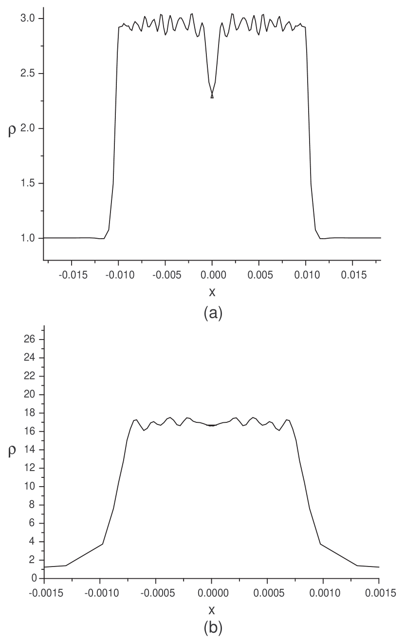
Figure 1: The density of (a) adiabatic and (b) isothermal shocks in which the MM97’s AV, equation (13), was used.

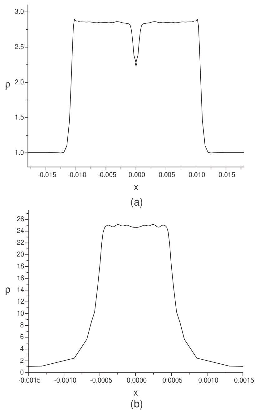
Figure 2: The density of (a) adiabatic and (b) isothermal shocks in which the time variable $\alpha$ and $\beta$ as outlined by equations (20) and (21), were used.

References

- (1) Balsara, D.S., 1995, J. Comp. Phys., 121, 357
- (2) Dyson, J.E., Williams, D.A., 1997, Physics of the Interstellar Medium, 2nd Edition, IOP publishing Ltd., p.99
- (3) Ellero, M., Serrano, M., Español, P., 2007, J. Comp. Phys., 226, 1731
- (4) Gingold, R.A., Monaghan, J.J., 1977, MNRAS, 181, 375
- (5) Gurzadyan, G.A., 1997, The Physics and Dynamics of Planetary Nebulae, Spriger-Verlag, Berlin, Heidelberg
- (6) Hernquist, L., Katz, N., 1989, ApJS, 70, 419
- (7) Koyama, H., Inutsuka, H.I., 2000, ApJ, 532, 980
- (8) Lanzafame, G., Belvedere, G., Molteni, D., 2006, A&A, 453, 1027
- (9) Liu, G.R., Liu, M.B., 2003, Smoothed Particle Hydrodynamics: A Meshfree Particle Method, World Scientific
- (10) Lucy, L.B., 1977, AJ, 82, 1013
- (11) Monaghan, J.J., 1989, J. Comp. Phys., 82, 1
- (12) Monaghan, J.J., 1992, ARA&A, 30, 543
- (13) Monaghan, J.J., 1994, J. Comp. Phys., 110, 399
- (14) Monaghan, J.J., 2005, Rep. Prog. Phys., 68, 1703
- (15) Monaghan, J.J., Gingold R.A., 1983, J. Comp. Phys., 52, 374
- (16) Morris, J.P., Monahgan, J.J., 1997, J. Comp. Phys., 136, 41