Theory of electric polarization induced by inhomogeneity in crystals

Abstract

We develop a general theory of electric polarization induced by inhomogeneity in crystals. We show that contributions to polarization can be classified in powers of the gradient of the order parameter. The zeroth order contribution reduces to the well-known result obtained by King-Smith and Vanderbilt for uniform systems. The first order contribution, when expressed in a two-point formula, takes the Chern-Simons 3-form of the vector potentials derived from the Bloch wave functions. Using the relation between polarization and charge density, we demonstrate our formula by studying charge fractionalization in a two-dimensional dimer model recently proposed.

Electric polarization is a fundamental quantity in condensed matter physics, essential to any proper description of dielectric phenomena of matter. Theoretically, it is well established that only the change in polarization has physical meaning and it can be quantified by using the Berry phase of the electronic wave functions King-Smith and Vanderbilt (1993); Resta (1994); Ortiz and Martin (1994). In practice, the Berry-phase formula is usually expressed in terms of the Bloch orbitals. It has been very successful in first-principles studies of dielectric properties of oxides and other insulating materials.

While the existing formulation is adequate in periodic insulators, a theory of polarization for inhomogeneous crystals would find numerous important applications; for example, in a class of recently discovered multiferroics, the appearance of electric polarization is always accompanied by long-wavelength magnetic structures Kimura et al. (2003); Hur et al. (2004); Lawes et al. (2005). A number of phenomenological and microscopic theories have been proposed to understand this magnetically induced polarization Lawes et al. (2005); Mostovoy (2006); Katsura et al. (2005); Sergienko et al. (2006); Hu ; however, quantitative studies of this type of problem still remain in a primitive state. The fundamental difficulty lies in the fact that the inhomogeneous ordering breaks the translational symmetry of the crystal so that Bloch’s theorem does not apply.

In this Letter we present a general framework to calculate electric polarization in crystals with inhomogeneous ordering. Our theory is based on the elementary relation between the change in polarization and integrated bulk current Resta (1994); Ortiz and Martin (1994). The latter can be evaluated using the semiclassical formalism of Bloch electron dynamics Sundaram and Niu (1999). We find that, in addition to the contribution previously obtained for uniform systems King-Smith and Vanderbilt (1993), the polarization contains an extra contribution proportional to the gradient of the order parameter. This extra contribution is expressed using the second Chern form of the Berry curvatures derived from the local Bloch functions. It can also be recast into a two-point formula, which depends only on the initial and final states, up to an uncertainty quantum after spatial averaging. We identify this quantum as the second Chern number in appropriate units. In addition, several general conditions for the inhomogeneity-induced polarization to be nonzero are also derived.

To demonstrate our theory, we apply our formula to study the problem of charge fractionalization in a two-dimensional dimer model recently proposed Seradjeh et al. ; Chamon et al. . We show that in this model fractional charge appears as a result of the ferroelectric domain walls. By using the relation between polarization and charge density, we calculate the total charge carried by a vortex in the dimerization pattern and compare it to previous results Seradjeh et al. ; Chamon et al. . Our approach has the advantage that it can be easily incorporated in a band calculation, while previously one relied on spectral analysis of the Dirac Hamiltonian performed in the continuum limit Seradjeh et al. ; Chamon et al. .

General formulation.—Suppose we have an insulating crystal with an order parameter $\bm{m}(\bm{r})$ that varies slowly in space. We assume that, at least on the mean-field level, $\bm{m}(\bm{r})$ can be treated as an external field that couples to an operator in the Hamiltonian $\mathcal{H}$. Thus, we can formally write $\mathcal{H}[\bm{m}(\bm{r})]$. As was emphasized in previous work King-Smith and Vanderbilt (1993); Resta (1994); Ortiz and Martin (1994), only the change in polarization $\bm{P}$ between two different states has meaning, and it is given by P-def

$$\bm{P}=\int_{0}^{T}dt\,\bm{j}(\bm{r},t)\;,$$ (1)

where $\bm{j}(\bm{r},t)$ is the bulk current density as the system adiabatically evolves from the initial state $(t=0)$ to the final state $(t=T)$. In other words, we assume that the two states are connected through a continuous transformation of the Hamiltonian $\mathcal{H}[\bm{m}(\bm{r});\lambda]$ parameterized by a scalar $\lambda$ with $\lambda(0)=0$ and $\lambda(T)=1$.

In order to find the current density $\bm{j}(\bm{r},t)$, we adopt the formalism of semiclassical dynamics of Bloch electrons Sundaram and Niu (1999), which is a powerful tool to investigate the influence of slowly varying perturbations on electron dynamics. Within this approach, each electron is described by a narrow wave packet localized around $\bm{r}_{c}$ and $\bm{k}_{c}$ in the phase space. If $\bm{m}(\bm{r})$ varies smoothly compared to the width of the wave packet, it is sufficient to study a family of local Hamiltonians $\mathcal{H}_{c}[\bm{m}(\bm{r}_{c});\lambda]$ which assumes a fixed value of the order parameter $\bm{m}(\bm{r}_{c})$ in the vicinity of $\bm{r}_{c}$. Since $\mathcal{H}_{c}[\bm{m}(\bm{r}_{c});\lambda]$ maintains the periodicity of the unperturbed crystal, its eigenstates have the Bloch form: $|\psi_{n}(\bm{k},\bm{r}_{c};\lambda)\rangle=e^{i\bm{k}\cdot\bm{r}}|u_{n}(\bm{k},\bm{r}_{c};\lambda)\rangle$, where $|u_{n}(\bm{k},\bm{r}_{c};\lambda)\rangle$ is the cell-periodic part of the Bloch functions. Note that the $\bm{r}_{c}$-dependence of $|u_{n}(\bm{k},\bm{r}_{c};\lambda)\rangle$ enters through $\bm{m}(\bm{r}_{c})$. We can then expand the wave packet using these local Bloch functions. For simplicity, in the following derivation we shall confine ourselves to the case of non-degenerate bands and hence omit the band index $n$.

It has been previously shown that the wave packet center satisfies the following equations of motion (hereafter the subscript $c$ on $\bm{k}_{c}$ and $\bm{r}_{c}$ is dropped) Sundaram and Niu (1999)

$$\dot{r}_{\alpha} =\nabla^{k}_{\alpha}\varepsilon-\Omega^{kr}_{\alpha\beta}\dot{r}_{\beta}-\Omega^{kk}_{\alpha\beta}\dot{k}_{\beta}-\dot{\lambda}\Omega^{k\lambda}_{\alpha}\;,$$ (2a)

$$\dot{k}_{\alpha} =-\nabla^{r}_{\alpha}\varepsilon+\Omega^{rr}_{\alpha\beta}\dot{r}_{\beta}+\Omega^{rk}_{\alpha\beta}\dot{k}_{\beta}+\dot{\lambda}\Omega^{r\lambda}_{\alpha}\;,$$ (2b)

where $\varepsilon$ is the electron energy and we have introduced the notation $\nabla^{k}_{\alpha}=\partial/\partial k_{\alpha}$ and $\nabla^{r}_{\alpha}=\partial/\partial r_{\alpha}$. Summation over repeated indices is implied throughout our derivation. Here, $\bm{\Omega}$ is the Berry curvature obtained from the vector potential $\bm{\mathcal{A}}$ derived from $|u(\bm{k},\bm{r},\lambda)\rangle$. For example,

$$\mathcal{A}^{k}_{\alpha}=\langle u|i\nabla^{k}_{\alpha}|u\rangle\;,\quad\mathcal{A}^{r}_{\alpha}=\langle u|i\nabla^{r}_{\alpha}|u\rangle\;,$$ (3)

$$\Omega^{kr}_{\alpha\beta}=\nabla^{k}_{\alpha}\mathcal{A}^{r}_{\beta}-\nabla^{r}_{\beta}\mathcal{A}^{k}_{\alpha}\;.$$ (4)

Other Berry curvatures are similarly defined. It is noteworthy that although the vector potential $\bm{\mathcal{A}}$ depends on the phase choice of the wave function $|u(\bm{k},\bm{r},\lambda)\rangle$, the Berry curvature $\bm{\Omega}$ is a well-defined gauge-invariant quantity in the parameter space $(\bm{k},\bm{r},\lambda)$.

We now turn to the derivation of $\bm{P}$ using Eq. (1). The electronic contribution to polarization is given by

$$\bm{P}=-e\int_{\text{BZ}}d\bm{k}\int_{0}^{T}dt\,D(\bm{k},\bm{r})\dot{\bm{r}}\;,$$ (5)

where $-e$ is the electron charge, and $D(\bm{r},\bm{k})$ is the electron density of states, which is modified from its usual value of $1/(2\pi)^{d}$ in the presence of the Berry curvature, $D(\bm{k},\bm{r})=(1+\Omega^{kr}_{\alpha\alpha})/(2\pi)^{d}$ Xiao et al. (2005).

We can solve $\dot{r}_{\alpha}$ from Eq. (2) then insert it into Eq. (5). Collecting terms proportional to $\dot{\lambda}$ and keeping those up to first order in the gradient, we obtain monopole

$$\bm{P}=\bm{P}^{(0)}+\bm{P}^{(1)}\;,$$ (6)

where $\bm{P}^{(0)}$ is the zeroth order contribution

$$P^{(0)}_{\alpha}=e\int_{\text{BZ}}\frac{d\bm{k}}{(2\pi)^{d}}\int_{0}^{1}d\lambda\,\Omega^{k\lambda}_{\alpha}\;,$$ (7)

and $\bm{P}^{(1)}$ is the first order contribution

$$\begin{split}P^{(1)}_{\alpha}&=e\int_{\text{BZ}}\frac{d\bm{k}}{(2\pi)^{d}}\int_{0}^{1}d\lambda\\ &\qquad\Bigl{(}\Omega^{kr}_{\beta\beta}\Omega^{k\lambda}_{\alpha}-\Omega^{kr}_{\alpha\beta}\Omega^{k\lambda}_{\beta}+\Omega^{kk}_{\alpha\beta}\Omega^{r\lambda}_{\beta}\Bigr{)}\;.\end{split}$$ (8)

These are the central results of this work. We note that $\bm{P}^{(0)}$ has been obtained by King-Smith and Vanderbilt for uniform systems King-Smith and Vanderbilt (1993), whereas $\bm{P}^{(1)}$, being proportional to the gradient of $\bm{m}(\bm{r})$, only exists in inhomogeneous crystals.

Two remarks are in order: firstly, although in the above derivation we have assumed an inhomogeneous order parameter, it is obvious that our theory is also applicable when the system is subject to a perturbation of a spatially-varying external field; secondly, we have only considered the electronic contribution to $\bm{P}$ here. When comparing with experiment, one should also include the ionic contribution, which is relatively easy to calculate because of its classical nature.

Two-point formula.—We first show that $\bm{P}^{(1)}$ has the desired property that it depends only on the initial and final states. The gauge-invariance of Eq. (8) allows us to evaluate it with any gauge choice. In order to carry out the integration over $\lambda$, we choose the path-independent gauge by requiring that the phase difference between $|u(\bm{k},\bm{r},\lambda)\rangle$ and $|u(\bm{k}+\bm{G},\bm{r},\lambda)\rangle$ does not depend on $\lambda$, where $\bm{G}$ is a reciprocal lattice vector Ortiz and Martin (1994). Under this gauge, Eq. (8) can be recast as CS

$$P^{(1)}_{\alpha}=e\int_{\text{BZ}}\frac{d\bm{k}}{(2\pi)^{d}}\Bigl{(}\mathcal{A}^{k}_{\alpha}\nabla^{r}_{\beta}\mathcal{A}^{k}_{\beta}+\mathcal{A}^{k}_{\beta}\nabla^{k}_{\alpha}\mathcal{A}^{r}_{\beta}+\mathcal{A}^{r}_{\beta}\nabla^{k}_{\beta}\mathcal{A}^{k}_{\alpha}\Bigr{)}\Big{|}_{0}^{1}\;.$$ (9)

We recognize that the integrand in the above equation is nothing but the Chern-Simons 3-form.

Table 1: Comparison between $\bm{P}^{(0)}$ and $\bm{P}^{(1)}$

	Two-point formula	Uncertain quantum
$\bm{P}^{(0)}$	Chern-Simons 1-form	First Chern number
$\bm{P}^{(1)}$	Chern-Simons 3-form	Second Chern number

However, we have paid a price for performing the $\lambda$-integration; namely, the spatially averaged polarization $\langle P^{(1)}_{\alpha}\rangle=(1/V)\int d\bm{r}P^{(1)}_{\alpha}$ resulting from this two-point formula (9) can only be determined modulo a quantum.

To find the size of the quantum, we consider a cyclic change in $\lambda$. Let us now assume that the order parameter $\bm{m}(\bm{r})$ is periodic in $\bm{r}$. The integral in Eq. (8) (after a spatial integration) over a closed manifold spanned by $(k_{\alpha},k_{\beta},r_{\beta},\lambda)$ is an integer called the second Chern number Avron et al. (1988). Since Eq. (9) does not track the evolution of $\lambda$, there is no information of how many cycles $\lambda$ has gone through. This is the reason why $\langle P^{(1)}_{\alpha}\rangle$ using Eq. (9) can only be determined modulo a quantum. Assuming $\bm{m}(\bm{r})$ depends on $y$, we obtain the quantum for $P^{(1)}_{x}$ in a three-dimensional system:

$$\Delta\langle P^{(1)}_{x}\rangle=\frac{e}{l_{y}a_{z}}\;,$$ (10)

where $l_{y}$ is the period of $\bm{m}(y)$ and $a_{z}$ is the lattice constant along $\hat{\bm{z}}$.

Similarly, the zeroth order contribution $\bm{P}^{(0)}$ can also be cast into a two-point formula and the uncertain quantum is given by $e/(a_{y}a_{z})$ King-Smith and Vanderbilt (1993). First-principles calculations show that in real materials $P^{(0)}$ is usually smaller than this quantum. Hence the ratio between $P^{(0)}$ and $P^{(1)}$ is roughly on the order of $l_{y}/a_{y}$. The similarities between $\bm{P}^{(0)}$ and $\bm{P}^{(1)}$ are summarized in Table 1.

Minimal conditions for a finite $\bm{P}^{(1)}$.—We now evaluate Eq. (8) using a particular path of $\lambda$. We write $\mathcal{H}[\bm{m}(\bm{r});\lambda]=\mathcal{H}[\lambda\bm{m}(\bm{r})]$ so that $\lambda$ acts like a “switch” of the order $\bm{m}(\bm{r})$, i.e., when $\lambda=0$ the system is orderless and when $\lambda=1$ the order is fully developed. Using the relation $\nabla^{r}_{\alpha}=\nabla^{r}_{\alpha}m_{\mu}\nabla^{m}_{\mu}$ and $\nabla^{\lambda}=(m_{\mu}/\lambda)\nabla^{m}_{\mu}$, we can recast Eq. (8) as

$$\begin{split}P^{(1)}_{\alpha}&=em_{\mu}\nabla^{r}_{\beta}m_{\nu}\int_{\text{BZ}}\frac{d\bm{k}}{(2\pi)^{d}}\int_{0}^{1}\frac{d\lambda}{\lambda}\\ &\qquad\Bigl{(}\Omega^{km}_{\alpha\mu}\Omega^{km}_{\beta\nu}-\Omega^{km}_{\alpha\nu}\Omega^{km}_{\beta\mu}+\Omega^{kk}_{\alpha\beta}\Omega^{mm}_{\mu\nu}\Bigr{)}\;.\end{split}$$ (11)

As we shall see below, this equation is very useful in assessing the general properties of $\bm{P}^{(1)}$.

Beside having the crystal be inhomogeneous, there are three general conditions for $\bm{P}^{(1)}$ to be nonzero according to Eq. (11): (i) the system must be two-dimensional or higher; (ii) the order parameter $\bm{m}(\bm{r})$ must have two or more components; and (iii) the wave function must depend on four or more independent parameters. These conditions can be obtained by realizing that the integrand in Eq. (11) is actually the second Chern 4-form $\Omega\wedge\Omega$ given in its local expression with respect to the coordinates $(k_{\alpha},k_{\beta},m_{\mu},m_{\nu})$. It is antisymmetric in $k_{\alpha}$ and $k_{\beta}$, and in $m_{\mu}$ and $m_{\nu}$, hence condition (i) and (ii). Condition (iii) follows from the fact that all 4-forms vanish identically in three or less dimensions. Based on condition (iii) we can further deduce that $\dim(\mathcal{H})>2$. If $\dim(\mathcal{H})=2$, $\mathcal{H}$ has four components. However, since shifting and scaling energy has no effect on wave functions, the wave function can depend on only two independent parameters (for example, the spherical coordinates on a 2-sphere $S^{2}$) and $\bm{P}^{(1)}$ vanishes in this case. This set of conditions puts powerful constraints on possible microscopic models that display finite $\bm{P}^{(1)}$. Conditions (i) and (iii) can also be obtained directly from Eq. (8).

Let us consider a two-dimensional “minimal” model and assume that both the space of $\bm{m}(\bm{r})$ and coordinate space are two-dimensional. Because of its antisymmetric properties, we can write the integrand of Eq. (11) as $\epsilon_{\alpha\beta}\epsilon_{\mu\nu}\chi$. Then Eq. (11) takes the following form

$$\bm{P}^{(1)}=e\chi[(\bm{\nabla}\cdot\bm{m})\bm{m}-(\bm{m}\cdot\bm{\nabla})\bm{m}]\;,$$ (12)

Here $\chi$, as a function of $\bm{m}(\bm{r})$, can be spatial dependent. Interestingly, if we identify $\bm{m}(\bm{r})$ with the magnetization order parameter $\bm{M}(\bm{r})$, the above result is consistent with the Landau-Ginzburg theory of polarization induced by spiral magnetic ordering Mostovoy (2006). However, our result (12) is a direct consequence of the minimal dimensionality and we did not invoke any symmetry analysis. For higher dimensions, one will have to carry out a careful symmetry analysis of the magnetic groups of the crystal Harris (2007).

Degenerate bands.—So far, our derivation is for non-degenerate bands. The generalization to degenerate bands is straightforward Culcer et al. (2005); Shindou and Imura (2005). The vector potential and Berry curvature become matrix-valued and are defined by

$$(\mathcal{A}_{a})_{mn}=\langle u_{m}|i\nabla_{a}|u_{n}\rangle\;,$$ (13)

$$\Omega_{ab}=\nabla_{a}\mathcal{A}_{b}-\nabla_{b}\mathcal{A}_{a}-i[\mathcal{A}_{a},\mathcal{A}_{b}]\;,$$ (14)

where $a,b\in(\bm{k},\bm{r},\lambda)$ and $|u_{m}\rangle$ and $|u_{n}\rangle$ are degenerate bands. We then need to take the trace of Eqs. (7) and (8) for the zeroth and first order contributions to $\bm{P}$. The two-point formula in Eq. (9) also takes the non-Abelian Chern-Simons form.

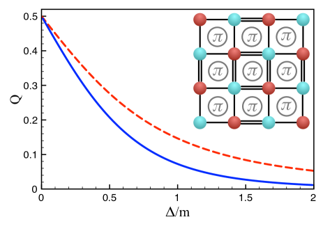
Figure 1: (color online). The total charge carried by the ferroelectric vortex domain wall $m(\bm{r})e^{i\theta}=m_{x}+im_{y}$ as a function of $\Delta/m$, where $\Delta$ is the staggered sublattice potential, and $m$ is the dimerization order parameter. As $\Delta$ increases, the difference between the result from the continuum limit (red dashed line) and that based on the band calculation (blue solid line) becomes significant. The insert shows the two-dimensional dimerized square lattice with $\pi$-flux per plaquette in the absence of the vortex. The hopping amplitude is $t(1\pm m_{x,y})$ along the $x,y$-direction.

Fractional charge.—To demonstrate our theory, we consider the problem of charge fractionalization in a recently proposed two-dimensional dimer model Seradjeh et al. ; Chamon et al. , shown schematically in the inset of Fig. 1. Introducing $\gamma_{i}=\sigma_{i}\otimes\sigma_{z}$, $\gamma_{4}=\openone\otimes\sigma_{x}$ and $\gamma_{5}=\openone\otimes\sigma_{y}$, we can write the Hamiltonian as $\mathcal{H}=h_{\alpha}\gamma_{a}$, where

$$\bm{h}=t(\cos k_{x},\cos k_{y},\Delta,m_{x}\sin k_{x},m_{y}\sin k_{y})\;,$$ (15)

$t\Delta$ is the staggered sublattice potential, $t(1\pm m_{x})$ and $t(1\pm m_{y})$ are the dimerized hopping amplitudes along $x$ and $y$ direction. We choose the Landau gauge so that the effect of the $\pi$ flux is represented by alternating signs of the hopping amplitudes along adjacent rows. It turns out that this model is a minimal one satisfying all our three conditions: (i) it is two-dimensional; (ii) the order parameter $\bm{m}=(m_{x},m_{y})$ has two components; and (iii) $\bm{h}$ (after scaling) can be mapped onto a unit sphere $S^{4}$ with four independent spherical angles.

It can be verified that the energy spectrum of this Hamiltonian consists of two doubly degenerate levels; therefore, the non-Abelian formalism is necessary. The Berry curvature has SU(2) symmetry Avron et al. (1988); Shankar and Mathur (1994); Demler and Zhang (1999); hence, $\bm{P}^{(0)}$ always vanishes since the non-Abelian version of Eq. (7) has vanishing trace. Thus, we will only consider $\bm{P}^{(1)}$ in what follows.

Suppose there is a vortex in the dimerization pattern: namely, $m_{x}+im_{y}=m(r)e^{in\theta}$. According to Eq. (12) together with the fact that $\rho(\bm{r})=-\bm{\nabla}\cdot\bm{P}$, this ferroelectric vortex domain wall will carry a polarization charge of $Q=\int d\bm{r}\rho(\bm{r})=nm^{2}\int_{0}^{2\pi}d\theta\,\chi$ Mostovoy (2006), which is in general fractional.

To compare with previous results, we shall first evaluate $\chi$ in the continuum limit. Expanding the Hamiltonian around the Dirac point $(\pi/2,\pi/2)$, we find, according to Eq. (11),

$$\chi=\frac{3}{2}n\int\frac{d\bm{k}}{(2\pi)^{2}}\int_{0}^{1}d\lambda\frac{\Delta\lambda}{(k^{2}+m^{2}\lambda^{2}+\Delta^{2})^{5/2}}\;.$$ (16)

Since at large $k$ the integrand decays as $k^{-5}$, we can extend the integration range of $\bm{k}$ to infinity and obtain

$$\chi=\frac{n}{4\pi m^{2}}(1-\frac{\Delta}{\sqrt{\Delta^{2}+m^{2}}})\;,$$ (17)

and the total charge carried by the vortex is given by

$$Q=n\frac{e}{2}(1-\frac{\Delta}{\sqrt{\Delta^{2}+m^{2}}})\;,$$ (18)

where $n$ is the winding number. This result agrees with the spectral analysis of the Dirac Hamiltonian Seradjeh et al. ; Chamon et al. .

The above derivation provides a simple picture of charge fractionalization in this type of system: it is a direct consequence of the ferroelectric domain wall, and the breaking of the sublattice symmetry ($\Delta$) allows it to be irrational. A detailed report including both 1D and 2D cases will be reported elsewhere. We also calculate the total charge based on a band calculation using Eq. (15), shown in Fig. 1. As $\Delta$ increases, the deviation between the band calculation and continuum limit becomes significant.

In summary, we have developed a general theory of polarization induced by inhomogeneity in crystals. Our result lays the foundation for quantitative studies of this type of problem. In connection to multiferroics, the minimal conditions for a finite $\bm{P}^{(1)}$ point to general directions to aid in the search for microscopic models. In addition, we have illustrated our theory by showing that the fractional charge in certain models can be understood as the polarization charge accompanying ferroelectric domain walls.

DX thanks D. Culcer for useful discussions. DX was supported by the NSF (DMR-0404252/0606485), JRS by the NSF of China (No. 10604063), DPC by DARPA (No. MDA0620110041), and QN by the Welch Foundation, DOE (DE-FG03-02ER45958), and the NSF of China (No. 10740420252).

References

- King-Smith and Vanderbilt (1993) R. D. King-Smith and D. Vanderbilt, Phys. Rev. B 47, 1651 (1993).
- Resta (1994) R. Resta, Rev. Mod. Phys. 66, 899 (1994).
- Ortiz and Martin (1994) G. Ortiz and R. M. Martin, Phys. Rev. B 49, 14202 (1994).
- Kimura et al. (2003) T. Kimura, T. Goto, H. Shintani, K. Ishizaka, T. Arima, and Y. Tokura, Nature 426, 55 (2003).
- Hur et al. (2004) N. Hur, S. Park, P. A. Sharma, J. S. Ahn, S. Guha, and S.-W. Cheong, Nature 429, 392 (2004).
- Lawes et al. (2005) G. Lawes, A. B. Harris, T. Kimura, N. Rogado, R. J. Cava, A. Aharony, O. Entin-Wohlman, T. Yildirim, M. Kenzelmann, C. Broholm, et al., Phys. Rev. Lett. 95, 087205 (2005).
- Mostovoy (2006) M. Mostovoy, Phys. Rev. Lett. 96, 067601 (2006).
- Katsura et al. (2005) H. Katsura, N. Nagaosa, and A. V. Balatsky, Phys. Rev. Lett. 95, 057205 (2005).
- Sergienko et al. (2006) I. A. Sergienko, C. Sen, and E. Dagotto, Phys. Rev. Lett. 97, 227204 (2006).
- (10) J. Hu, eprint arXiv:0705.0955.
- Sundaram and Niu (1999) G. Sundaram and Q. Niu, Phys. Rev. B 59, 14915 (1999).
- (12) B. Seradjeh, C. Weeks, and M. Franz, eprint arXiv:0706.1559.
- (13) C. Chamon, C.-Y. Hou, R. Jackiw, C. Mudry, S.-Y. Pi, and A. P. Schnyder, eprint arXiv:0707.0293.
- (14) Strictly speaking, there is still an ambiguity in the definition of given here because also contains a contribution from the magnetization current. As a result, is only defined up to a divergence-free field. One can of course fix the gauge by imposing that only have a longitudinal component. However, this is not a critical issue because the ambiguity can be removed by spatial averaging.
- Xiao et al. (2005) D. Xiao, J. Shi, and Q. Niu, Phys. Rev. Lett. 95, 137204 (2005).
- (16) The integral of terms that do not contain is given by . The integral of over the entire Brillouin zone obviously vanishes. After integration by parts and making use of the Bianchi identity , one can show that the integral of the last three terms contributes a divergence-free part, which can be discarded.
- (17) The formal derivation of Eq. (9) is lengthy and will be reported elsewhere. In the simplest case where is well-defined everywhere in , one can prove Eq. (9) by using Stokes’ theorem .
- Avron et al. (1988) J. E. Avron, L. Sadun, J. Segert, and B. Simon, Phys. Rev. Lett. 61, 1329 (1988).
- Harris (2007) A. B. Harris, Phys. Rev. B 76, 054447 (2007).
- Culcer et al. (2005) D. Culcer, Y. Yao, and Q. Niu, Phys. Rev. B 72, 085110 (2005).
- Shindou and Imura (2005) R. Shindou and K.-I. Imura, Nucl. Phys. B 720, 399 (2005).
- Shankar and Mathur (1994) R. Shankar and H. Mathur, Phys. Rev. Lett. 73, 1565 (1994).
- Demler and Zhang (1999) E. Demler and S.-C. Zhang, Ann. Phys. 271, 83 (1999).