When GRB afterglows get softer, hard components come into play

Abstract

Aims. We aim to investigate the ability of simple spectral models to describe the GRB early afterglow emission.

Methods. We performed a time resolved spectral analysis of a bright GRB sample detected by the Swift Burst Alert Telescope and promptly observed by the Swift X–ray Telescope,with spectroscopically measured redshift in the period April 2005 – January 2007. The sample consists of 22 GRBs and a total of 214 spectra. We restricted our analysis to the softest spectra sub–sample which consists of 13 spectra with photon index $>$ 3.

Results. In this sample we found that four spectra, belonging to GRB060502A, GRB060729, GRB060904B, GRB061110A prompt–afterglow transition phase, cannot be modeled neither by a single power law nor by the Band model. Instead we find that the data present high energy ($>$ 3 keV, in the observer frame) excesses with respect to these models. We estimated the joint statistical significance of these excesses at the level of 4.3 $\sigma$. In all four cases, the deviations can be modeled well by adding either a second power law or a blackbody component to the usual synchrotron power law spectrum. The additional power law would be explained by the emerging of the afterglow, while the blackbody could be interpreted as the photospheric emission from X–ray flares or as the shock breakout emission. In one case these models leave a 2.2$\sigma$ excess which can be fit by a Gaussian line at the energy the highly ionized Nickel recombination.

Conclusions. Although the data do not allow an unequivocal interpretation, the importance of this analysis consists in the fact that we show that a simple power law model or a Band model are insufficient to describe the X-ray spectra of a small homogeneous sample of GRBs at the end of their prompt phase.

1 Introduction

The X-ray telescope (XRT, Burrows et al., (2005)) on board the Swift satellite (Gehrels et al. (2004)) allows to perform time resolved spectroscopy of a large number of gamma ray burst (GRB) afterglows in the 0.3-10 keV energy band. The vast majority of the spectra can be modeled by a single absorbed power law (SPL) model. In most of the afterglows a strong spectral evolution is observed in the early phases with spectral indexes varying in the range 0.5-5 (O’Brien et al. (2006),Butler 2007a , Zhang et al. (2007)). These observations are consistent with the classical fireball model which describes the burst and afterglow emission due to synchrotron radiation.

Figure 1: The 13 very soft spectra are shown together with their best SPL fit. They are sorted in time from the top-left corner. The observed time interval and the photon index are indicated in the figures. The asterisks denote the four spectra for which we found significant departures from SPL model.

It is possible that detection of different spectral features, signature of other emission mechanisms, like thermal components or recombination lines might give some insight about GRB progenitors, chemical composition, physical conditions and geometry of the GRB environment. Before the Swift mission, several X–ray line detections were reported in GRB late ($>$ 10 hr) afterglow observations. The statistical significance of these detections has been questioned by Sako et al. (2005), who concluded that there were no credible X–ray features in any GRB afterglow. Butler et al. (2005), however, showed that for GRB011211 the different estimates of the statistical significance can be explained by the different approach in the continuum modelling.

In the Swift afterglow observations only a few deviations from SPL have been reported. Most of them have been explained by the curvature of the synchrotron spectrum and the presence of the $\nu F_{\nu}$ peak (E_peak) within the XRT band (Falcone et al. 2006, Butler & Kocevski 2007, Goad et al. 2007, Mangano et al. 2007, Godet 2007a).

Moreover Butler (2007) found anomalous soft X-ray emission in the spectra of four GRBs which can be interpreted as multiple emission lines due to K shell transition in light metals as well as thermal emission from a blackbody with temperature $\sim$0.1 keV. Grupe et al. (2007) and Godet et al. (2007a) found that early afterglow data of GRB060729 and GRB050822, respectively, can be fitted with a SPL plus a blackbody with decreasing temperature in the first few hundreds seconds from the beginning of the prompt emission. Campana et al. (2006) found a cooling thermal component in the spectrum of SN2006aj/XRF060218, interpreted as due to the supernova shock break-out (this interpretation has been subsequently questioned by Li 2007 and Ghisellini et al. 2007).

Starting from the idea that any deviation from a SPL spectral model, if present, would be a faint signal mostly covered by the high level “noise” of synchrotron emission, we searched for the best observational conditions to detect it. In particular, we searched for high energy excesses with respect to the SPL when the spectrum is steepest and, at least in the hard part of the energy band, could be the non dominating component.

Throughout this paper, all errors are quoted at 68% confidence level for one parameter of interest, unless otherwise specified. The reduced $\chi^{2}$ will be denoted as $\chi^{2}_{\nu}$ and the number of degrees of freedom with the abbreviation “d.o.f.”. We follow the convention $F_{\nu}(\nu,t)\propto t^{-\alpha}\nu^{-\beta}$, where $\alpha$ and $\beta$ are the temporal decay slope and the spectral index, respectively. As time origin, we will adopt the Burst Alert Telescope (BAT) trigger (T0). The photon index is $\Gamma=1+\beta$. Last, we adopt the standard “concordance” cosmology parameters, $\Omega_{\rm m}=0.27$, $\Omega_{\Lambda}=0.73$, $h_{0}=0.71$.

2 Data analysis and sample selection

We considered the GRB sample detected by BAT, promptly observed by XRT in the period April 2005–January 2007 which collected at least 800 photons. We restricted our analysis to the sample with spectroscopically measured redshift in order to separate the local contribution to the total absorbing column from the Galactic one. We excluded GRB060218 from our analysis because of its peculiarity (Campana et al. (2006)). For each burst, when possible, we split the XRT data in different time intervals in such a way that in each of them there are 2000 photons, before the background subtraction (the last spectrum collects the remaining photons). The final sample consists of 22 bursts for a total of 214 time intervals. The data reduction was performed using the standard software (HEADAS software, v6.1, CALDB version Jul07) and following the procedures reported in the instrument user guides. The spectral analysis was performed using XSPEC (v11.3). The 214 spectra were binned in order to ensure a minimum of 20 counts per energy bin, ignoring channels below 0.3 keV and above 10 keV. For the Galactic hydrogen column density $N_{\rm H,MW}$ we assumed the value reported in Dickey & Lockman (1990) along the GRB direction. We multiplied to the spectral models an extra neutral absorber at the source redshift letting the column density $N_{{\rm H},z}$ free to vary. SPL provided very good fits in most cases and we found that the photon index $\Gamma$ ranges from 0.5 to 3.9. In particular there are 13 spectra (6% of the total), belonging to 5 different bursts with $\Gamma>$3 . These are: one from GRB 060502A, GRB 060614 and GRB 060904B, three from GRB 061110A and seven from GRB 060729. They are all collected in Windowed Timing (WT) mode (see Hill et al. 2004 for a description of the different operational modes of the XRT) and belong to the prompt–afterglow transition phase, observed less than 500 seconds after the event triggers. In Fig. 1 the 13 very soft spectra are shown together with their best SPL fit. The mean $\chi^{2}_{\nu}$ value of this 13 spectra sub-sample is 1.20$\pm$0.07, significantly worse than the average of the entire sample that is 1.01$\pm$0.01 (chance probability $<$10^-4). In particular there are some evident departures from SPL model at high energies in four spectra from four bursts.

3 Excess statistical significance

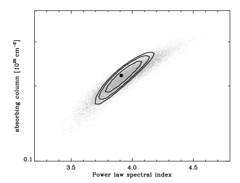
Figure 2: Black point and black contour are the best fit and 1,2,3 $\sigma$ confidence contour of the fit on one observed spectrum of GRB 060729. Grey dots are the best fit results on a sample of 20,000 simulated spectra.

Having in mind the rules of thumb given by Protassov et al. (2002), to determine if there are statistically significant departures from SPL, we followed step by step the method described by Rutledge & Sako (2003) which was used to calculate the significance of many X-ray features by Sako et al. (2005).

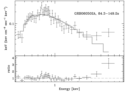
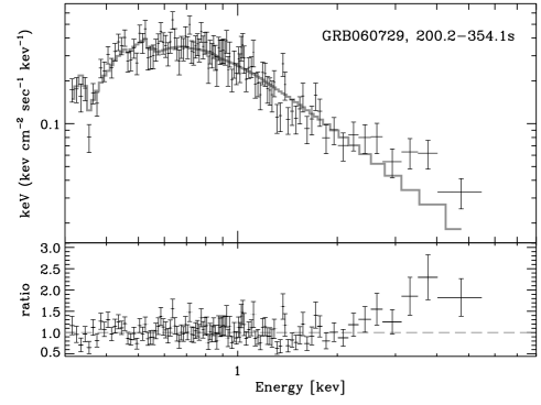
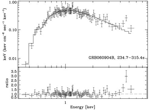
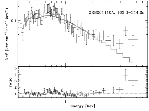
Figure 3: The spectra (in energy units) of the four GRB afterglows for which we detect significant departures from SPL model which is plotted in grey.

First, we considered the redistribution matrix (RMF=RMF(PI,E)) and we fitted each column of the matrix (2400 in total; see) by a Gaussian function. As done by Rutledge & Sako (2003) we built a new RMF with the 2400 columns replaced by the Gaussian fit of the original RMF. Because our features are broader than the instrumental spectral resolution (which is 0.11 keV at 4 keV) we also built four artificial RMFs with Gaussian functions 3,5,10,16 times wider than the best fit of the original RMF value. In practice, we built a set of 4 different RMF worsening the spectral resolution to look for the scale which maximizes the signal-to-noise ratio.

For each of the 13 spectra being tested, we convolved the PI count spectrum with the 5 (1 nominal, 4 smoothed) RMFs. Then, for each of the 13 observed spectra, we created 100,000 Montecarlo (MC) realizations of the raw pulse-invariant (PI) spectra based on the respective best-fit SPL models using a fixed number of source plus background photons. Background events were randomly selected from a background spectral model, derived from fits to spectra obtained from a source–free region of a deep exposure.

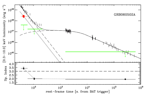
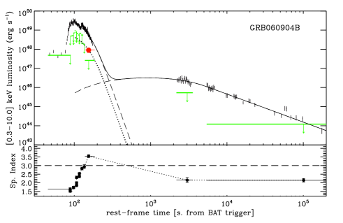
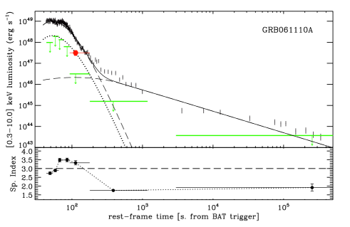
Figure 4: Upper panels: The luminosity (0.3-10 keV rest–frame energy band) curves of the four GRB afterglows for which we detect significant departures from SPL model. With the continuous lines we plot the best fit using the model described by Willingale et al. (2007), split in prompt and afterglow contributions (dashed lines). With the filled circles we plot the luminosity of the spectral excesses we detect. The upper limits to the detection of the extra components (see Section 4) in the different time slices are also reported as top-down arrows (for the clarity of the picture we report only the value calculated assuming a DPL model, see Section 4). With the dotted line we plot the fit of the prompt emission re-normalized to the luminosity of the extra component. Lower panels: The spectral indexes $\Gamma$ given by SPL fit, measured in the different time slices.

To check the accuracy of our MC simulations for each GRB we ran the XSPEC grouping and fit procedures on a sample of 20,000 simulated spectra. In Fig. 2 for one spectrum of GRB060729 we compare the results of the SPL model fit of the observed data, with the results of the fit on simulated data.

As we did for the observed data, we convolved all the 100,000 simulated PI spectra with the 5 matrices corresponding to the 5 filter scales. For each spectrum and each scale we counted the number of MC realizations exceeding the feature in the data and recording the energy and the scale for which this number is minimum. There are four spectra, in the sample of 13, for which we found excesses in the data that can be reproduced as statistical fluctuations of the SPL in less than 10 trials out of 100,000. This correspond to a single trial significance higher than 99.99% . These are the last WT spectra, coinciding with the last phase of the X–ray light curve steep decay, of GRB 060502A, 060729, 060904B and 061110A (Table 1 and Fig. 3, 4). In the rest of the paper we will limit our analysis to these four spectra.

Table 1: (I) GRB: Name of the GRB; (II) Rest–frame time interval; (III) Redshift; (IV) energy of the excess maximum (observer frame); (V) energy scale in times of instrumental resolution (VI) Single trial significance; (VII) Multi trial significance. Ref: ¹La Parola (2006); ²Cucchiara et al. (2006); ³Grupe et al. (2007); ⁴Thoene et al (2006a); ⁵Grupe et al. (2006); ⁶Fugazza et al. (2006); ⁷Fox et al. (2006); ⁸Thoene et al (2006b).

GRB	$\Delta$t	z	E	Sc.	s.t.	m.t.
	s		keV		(%)	(%)
060502A1	33-59	1.512	5.7	7	99.9932	99.4778
0607293	130-230	0.544	3.7	10	99.9875	99.0421
060904B5	138-185	0.7036	4.6	3	99.9993	99.9461
061110A7	93-179	0.7578	4.7	5	99.9997	99.9769

In order to improve the accuracy in the calculation of the excess statistical significance, for the sample of four spectra we enlarged the simulated sample to 1,000,000. Results are reported in Table 1 and illustrated in Fig. 5. We note that in the case of GRB 060729, with 1,000,000 MC tests we obtained a significance value slightly lower than the one we obtained with 100,000 tests and slightly lower than the 99.99% threshold (99.9875%). Because the two results are perfectly consistent (within $1\sigma$ errors) we kept GRB 060729 in our sample.

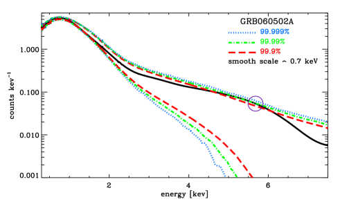
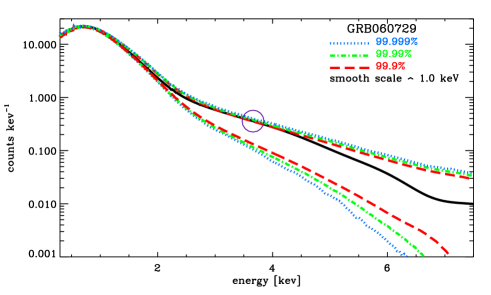
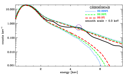
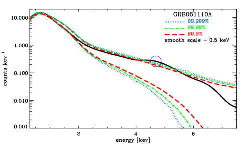
Figure 5: Data are compared with the single trial confidence contours as resulted from MC simulations (10⁶ tests for each GRB; see Tab.1). In the plot, data and simulations contours are both smoothed to the energy resolution scale which maximizes the spectral feature signal. These are 7, 10, 3 and 5 times the instrumental spectral resolution, approximately corresponding to 0.7, 1.0, 0.3, 0.5 keV respectively for the four afterglows (note that energy resolution varies within the XRT energy band so these are only rough estimates). The circles indicate where the most significant excess is detected.

To calculate the corresponding multi-trial significance, we took into account that we searched for excesses on a sample of 13 spectra on five different energy resolution scales. For each energy scale we considered a different number of energy resolution elements: 40,14,8,4,3 respectively for the 1,3,5,10,16 scales. The results are reported in Table 1. Because we searched for features on a homogeneous sample of 13 spectra, resulting in 4 successes, we can also estimate the joint statistical significance. In particular, we set a lower limit to the total joint probability using the binomial distribution and assuming that all the four spectra have the same multi-trial significance equal to the lowest (P=99.04%). Then we searched for the probability to have a rate of 4 successes out of 13 tests with mean probability P, resulting in a joint significance of 99.9994% ($4.3\sigma$) which ensures that the features we detected cannot be explained as statistical fluctuations beyond any reasonable doubt.

Table 2: (I)GRB: Name of the GRB; (II)Model: fitting model (see text); (III)$N_{{\rm H},z}$: neutral absorber column density at the source redshift; (IV)$\Gamma_{1}$, ($\Gamma_{2}$): photon index of the first (second, present if model is DPL) power law; second photon index is fixed to the value of the late afterglow; (V)E: rest frame blackbody temperature if Model is BB1, or BB2 or mean value of the Gaussian line if model is GAU; (VI)R_b: blackbody radius; (VII)$\sigma_{g}$: $\sigma$ of the Gaussian line; (VIII)L: unabsorbed luminosity of the extra component in the rest–frame [0.3-10] keV energy band; (IX)$\chi^{2}$(dof): reduced $\chi^{2}$ (degrees of freedom) in two different energy bands.

GRB	Mod	$N_{{\rm H},z}$	$\Gamma_{1}$, ($\Gamma_{2}$)	E	Rb	$\sigma_{g}$	L	$\chi^{2}$(dof)
		$10^{22}$cm-2		keV	cm	keV	1047erg s-1	0.3-10keV, 1-10keV
060502A	SPL	0.63${}_{-0.11}^{+0.12}$	3.39${}_{-0.16}^{+0.18}$	–	–	–	575.$\pm$33.0	1.29(36), 2.03(11)
	DPL	1.26${}_{-0.21}^{+0.23}$	4.97${}_{-0.42}^{+0.44}$, (1.99)	–	–	–	39.8$\pm$8.50	0.81(35), 0.61(10)
	BB1	0.41${}_{-0.16}^{+0.18}$	2.22${}_{-0.28}^{+0.28}$	0.33${}_{-0.03}^{+0.03}$	7.3${}_{-0.8}^{+2.1}$1012	–	83.1$\pm$11.1	0.72(34), 0.70(9)
	BB2	1.02${}_{-0.17}^{+0.19}$	4.16${}_{-0.30}^{+0.33}$	3.24${}_{-0.80}^{+2.27}$	2.2${}_{-0.7}^{+1.9}$1010	–	7.23$\pm$1.45	0.80(34), 0.72(9)
	GAU	1.04${}_{-0.18}^{+0.17}$	4.20${}_{-0.33}^{+0.27}$	1.03${}_{-1.03}^{+8.97}$	–	8.8${}_{-4.8}^{+0.2}$	7.88$\pm$1.61	0.82(33), 0.80(8)
060729	SPL	0.22${}_{-0.02}^{+0.02}$	3.91${}_{-0.10}^{+0.10}$	–	–	–	77.2$\pm$2.50	1.24(105), 1.60(38)
	DPL	0.32${}_{-0.03}^{+0.03}$	4.63${}_{-0.19}^{+0.20}$, (1.94)	–	–	–	2.28$\pm$0.39	1.05(104), 1.14(37)
	BB1	0.07${}_{-0.04}^{+0.04}$	2.94${}_{-0.20}^{+0.20}$	0.20${}_{-0.02}^{+0.02}$	6.4${}_{-0.8}^{+5.9}$1012	–	8.62$\pm$0.84	1.01(103), 1.08(36)
	BB2	0.32${}_{-0.03}^{+0.04}$	4.54${}_{-0.19}^{+0.21}$	1.25${}_{-0.15}^{+0.22}$	5.6${}_{-0.9}^{+1.2}$1010	–	1.01$\pm$0.16	1.03(103), 1.08(36)
	GAU	0.30${}_{-0.03}^{+0.04}$	4.40${}_{-0.19}^{+0.25}$	3.75${}_{-2.75}^{+1.07}$	–	2.0${}_{-0.6}^{+1.4}$	0.76$\pm$0.12	1.03(102), 1.09(35)
060904B	SPL	0.69${}_{-0.04}^{+0.04}$	3.55${}_{-0.08}^{+0.08}$	–	–	–	329.$\pm$0.08	1.00(103), 1.12(60)
	DPL	0.86${}_{-0.07}^{+0.08}$	4.22${}_{-0.23}^{+0.23}$, (2.15)	–	–	–	15.2$\pm$2.90	0.92(102), 0.98(59)
	BB1	0.50${}_{-0.09}^{+0.10}$	2.91${}_{-0.26}^{+0.24}$	0.30${}_{-0.03}^{+0.03}$	4.9${}_{-0.6}^{+0.6}$1012	–	25.2$\pm$3.50	0.93(101), 0.97(58)
	BB2	0.79${}_{-0.06}^{+0.06}$	3.84${}_{-0.14}^{+0.16}$	3.02${}_{-1.03}^{+5.98}$	1.4${}_{-0.6}^{+3.5}$1010	–	2.22$\pm$0.39	0.91(101), 0.96(58)
	GAU	0.74${}_{-0.05}^{+0.05}$	3.67${}_{-0.09}^{+0.10}$	7.85${}_{-0.25}^{+0.16}$	–	0.5${}_{-0.2}^{+0.3}$	1.10$\pm$0.18	0.87(100), 0.90(57)
061110A	SPL	0.13${}_{-0.03}^{+0.04}$	3.32${}_{-0.12}^{+0.13}$	–	–	–	40.6$\pm$1.60	1.74(77), 2.54(26)
	DPL	0.45${}_{-0.07}^{+0.07}$	4.99${}_{-0.29}^{+0.30}$, (1.75)	–	–	–	4.23$\pm$0.59	1.16(76), 0.99(25)
	BB1	0.03${}_{-0.03}^{+0.05}$	2.17${}_{-0.17}^{+0.17}$	0.23${}_{-0.02}^{+0.01}$	5.1${}_{-0.3}^{+0.6}$1012	–	9.49$\pm$0.82	1.07(75), 1.07(24)
	BB2	0.37${}_{-0.06}^{+0.06}$	4.40${}_{-0.25}^{+0.27}$	1.82${}_{-0.25}^{+0.36}$	3.6${}_{-0.6}^{+0.9}$1010	–	1.86$\pm$0.25	1.18(75), 1.24(24)
	GAU	0.34${}_{-0.04}^{+0.07}$	4.29${}_{-0.17}^{+0.26}$	1.00${}_{-0.25}^{+0.36}$	–	5.2${}_{-1.0}^{+0.8}$	1.89$\pm$0.26	1.20(74), 1.33(23)

3.1 Instrumental effects

We investigated the possibility that these features are produced by some instrumental effects such as pile–up. This cannot be the case, because the mean count rate in all the four cases is less than 33 counts s^-1 and it is always below 70 counts s^-1, a factor 3 below the pile–up threshold in WT ($\sim$ 200 counts s^-1, see Campana et al. 2008). We can also exclude that these features are produced by some anomalous hot pixels from the comparison with the expected point spread function (Moretti et al. (2005)).

We can also exclude that the excesses are due to uncertainties in the instrument response calibration. All the excesses are found at energies $>$ 3.5 keV (Table 1) in the central part of the CCD ($<$ 70 pixels, equivalent to $\sim$ 3 arcmin). In this position and energy range the systematics in the effective area, quantum efficiency and energy redistribution calibrations are less than 5%. (see and Godet et al. 2007b). In fact all the major instrumental edges are below 3.5 keV (Au for the mirror, Al for the filter, C, N, O and Si for the CCD) and there is no evidence of position dependence at energies higher than 0.5 keV.

The excesses cannot result from the background subtraction procedure. In fact, the expected background events, in the extraction region we considered, in 100 second exposure, is 1.2$\pm$0.2; among them 0.6 are expected with energy higher than 2 keV (Moretti et al. 2007). Moreover, we checked our data against uncovered anomalies performing our analysis with different background extraction regions and we found perfectly consistent results.

In the case of GRB060904B, a galaxy cluster with a core radius of 12 arcsec is present in foreground, at 2.3 arcminutes of projected distance from the GRB. By modeling the cluster surface brightness with a King profile in the extraction region of the afterglow we expect to find $<$1 photon (99.99% confidence) from the cluster in the 80 s exposure.

4 Modeling the data with an extra component

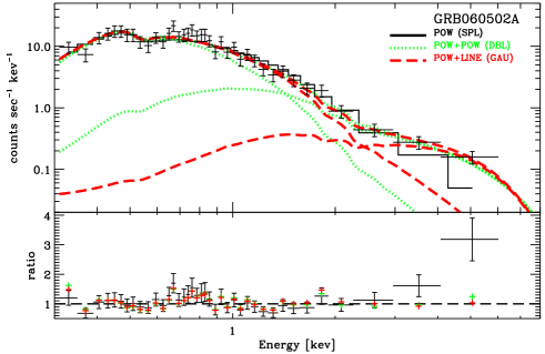
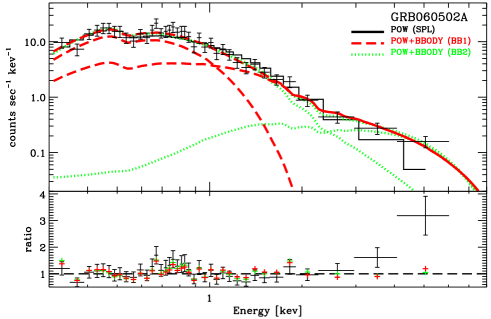
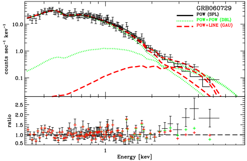
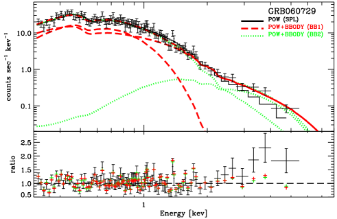
Figure 6: The anomalous spectra in the GRB 060502A and GRB060729 afterglows. For the sake of clarity, we use two plots for each spectrum: we plot DPL (dotted grey line) and GAU (dashed line) on the left plots and BB1 (dashed line) and BB2 (dotted grey line) on the right plots. In each plot we show the contribution of the single components and their sum, with the same line style and color. SPL best models are plotted with the continuous black step-line. In the lower panels of each plot we show the ratio between data and models with the same color code. For the sake of clarity we plot errors only for SPL models

As discussed in the previous section we found a sub-sample of four spectra, belonging to four different GRB which present highly significant deviations from the SPL models. In fact, if fitted with SPL, they all four present a clear excess at high energies.

As already said, most of the departures from SPL models found in time resolved spectral analysis of Swift observations of early afterglow have been explained so far by the curvature of the spectrum and the presence of the $\nu F_{\nu}$ peak (E_peak) within the XRT band (Falcone et al. 2006, Butler & Kocevski 2007, Goad et al. 2007, Mangano et al. 2007). The four spectra we are considering can be modeled neither by a Band model (Band et al. 1993) nor by a power law with an exponential cutoff. In the time intervals we are considering, the BAT signal is almost null. This prevented us from studying the spectrum in the combined energy band. However, any attempt at fitting the XRT spectra with a cutoff power law or with a Band model could not constrain the E_peak within the XRT band and therefore did not improve the SPL fit. We found that our analysis is consistent with previous papers. In particular Butler & Kocevski (2007) performed time resolved spectroscopic analysis of BAT and XRT simultaneous observations of a large sample of Swift GRBs. For GRB 060729 and GRB 060904B, in particular, they found that, during the early phases of the afterglow, the energy peak (E_peak) of the prompt emission spectrum transits in the X-ray band. The time intervals where we observe excesses in the spectrum of GRB 060904B (Table 1) roughly correspond to the last 5 temporal bins of their analysis (240-315 seconds in the observer frame). Although they do not explicitly report the best fit parameter and the $\chi^{2}$ values, it is clear from their Fig. 9 (third panel from the top on the right) that while the Band model is a good description of the data at the beginning of the XRT observation, in these five particular intervals, Band model gives a very poor description of the data, always leaving one parameter unconstrained. The same conclusion can be also drawn for GRB 060729, where our time interval corresponds to their last three time slices. We also note that for this GRB the same conclusion is also confirmed by Grupe et al. (2007) who found that cutoff power law model gives $\chi^{2}_{\nu}$ values larger than 1.5 in the same time interval.

Therefore we tried to fit the data adding three different components to the SPL: (i) a second power law component with the slope frozen to the value of the late afterglow spectrum letting only the normalization vary (DPL); (ii) a blackbody; (iii) a Gaussian line (GAU). As it will be explained later (Sect. 5.3), we found that, with the blackbody model, two equally good fits could be found with quite distinct parameter values. Therefore we considered a blackbody with temperature varying in the 0.1-10 keV energy band with initial guess kT=0.2 keV (BB1) and kT=2 keV (BB2). . The results are reported in Table 2 and shown in (Fig. 6-7).

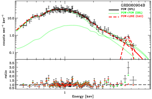
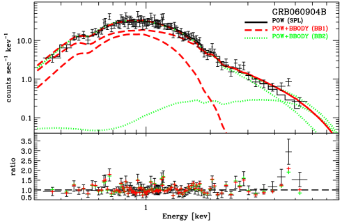
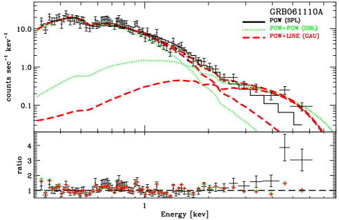
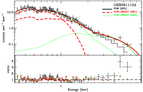
Figure 7: Same of Fig. 6, for GRB 060904B and GRB061110A afterglow anomalous spectra.

5 Discussion

5.1 Energetics and time variability of the spectral features

The DPL, BB2 provided an extra component to SPL which compensates the high energy residuals. In BB1 models, the blackbody component represents a significant fraction of the softer part of the spectrum, while the excesses at high energies are accounted for by the power law component. The (unabsorbed) luminosities of the additional components calculated in the [0.3-10] keV rest–frame energy band are typically 1–10% of the total, in DPL, BB2 and GAU models, while it is 10–20% of the total in BB2 models (Table 2 and (Fig. 6-7)). As illustrated in Fig. 4 for all the four afterglows we could perform time resolved spectroscopy. The time intervals from which we extracted the anomalous spectra correspond to the last WT spectrum, right before the canonical steep–shallow light–curve break (Nousek et al. (2006)). With the same criteria adopted for the original 13 very soft spectra we did not find any other significant deviation from SPL model in any of the time slices considered. In order to study the time variability of the spectral features, for each of the four GRBs, we estimated the detection upper limits. To do this, for each slice, we added an extra component (second power law, blackbody and Gaussian) with the parameter value set to the best DPL, BB1, BB2 and GAU values, letting the normalization free to vary. We set the upper limits for the detection when these additional components produce a factor of 3 worsening in terms of null hypothesis probability of the $\chi^{2}_{\nu}$ of the SPL fit. We note that this should be considered as a rough estimate of the upper limits; a rigorous calculation of all the upper limits would have required an unrealizable number of simulations. However we verified that, at least in one case, the upper limits roughly calculated differs by less than 30% from the one rigorously calculated.

The upper limits vary during the afterglow depending on the flux and on the softness of the spectrum. In particular, as shown in Fig. 4, the detection of the spectral features, in the last spectrum before the plateau phase, coincides with a drop of the detection threshold. This is due to the simultaneous flux decay and spectral softening which allow the detection of spectral features in the higher part of the energy band. We note that GRB 060904B did not show this component at early times, although the sensitivity was also good then. We also note that in at least three cases the extra components present in the last part of the light curve steep decay disappear in the shallow phase, although the upper limits in this time slices are very low (in the case of GRB 060904B, the observation stopped during the steep decay of a giant X–ray flares). Evidently, whatever its nature, the emission mechanism responsible for these spectral features varies on a time scale similar to the prompt emission.

5.2 Double power law (DPL)

In three cases DPL model provides the best improvement in the fit, taking into account that we add only one extra parameter to the SPL model. This model would provide a natural explanation to the excesses we observe. In fact, because the afterglow spectrum is significantly harder than the prompt tails, when the prompt flux decreases and softens, the afterglow emission becomes visible at higher energies. This would easily explain the fact that the excesses are detected just before the steep-shallow light–curve break and disappear in the following time slice. On the other hand, as shown in Fig. 4, the excess luminosity is much larger than the expected contribution of the afterglow forward shock component alone (e.g. Sari (1997), Willingale et al. 2007). But it might be explained by the radiation produced by an extreme reverse shock in the X–ray band (see Zhang et al. 2006, Kobayashi & Zhang 2007).

5.3 Power law plus blackbody (BB1, BB2)

Good fits are also provided by adding to the SPL a blackbody component (2 extra parameters). In all the four afterglows, with this model, the fit results depend on the blackbody temperature initial guess. As shown in Fig. 8, $\chi^{2}$ has two (and only two) different but equally significant minima. BB1, with initial guess kT=0.2 keV, gives good fits with (redshift-corrected) temperatures in the range 0.20–0.33 keV, radii in the range (4.9–7.3)$\times$10¹² cm and power law indexes in the range 2.2–2.9. BB2, with initial guess kT=2 keV gives good fits with red–shift corrected temperatures in the range 1.3–3.2 keV, radii in the range (1.4–5.6)$\times$10¹⁰ cm and power law indexes in the range 3.8–4.5. For GRB 060502A and GRB 061110A, BB1 fits provided slightly better $\chi^{2}$ as calculated on the whole energy band, while for GRB 060729 and GRB 060904B the fits yield equivalent results. Interestingly, in each of the four cases, the $\chi^{2}$ matrix projection on the photon index – temperature parameter plane has always two well defined minima which are split in two different regions of the plane (Fig. 8). This explains why fit results depend on the initial guess value of the blackbody temperature.

In the case of GRB 060729 our BB1 model is consistent with the results of Grupe et al. (2007) and Godet (2007a). They interpreted the thermal emission as due to the photospheric emission from X–ray flares. In fact, assuming that X–ray flares, in the early afterglow, are produced by the same mechanism of the prompt phase, a thermal component in the early afterglow spectra is expected in a similar way to the prompt emission (Ryde et al 2006). This interpretation can be easily extended to the other three GRBs that have very similar characteristics.

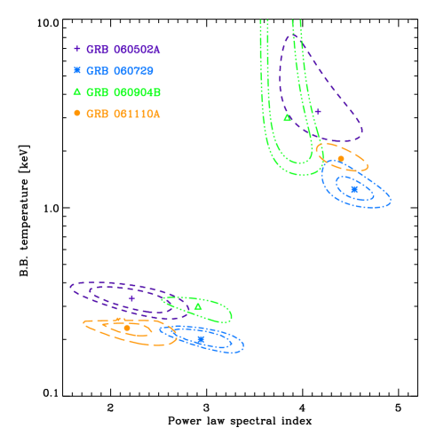
Figure 8: Confidence contours (68% and 90%) of the single power law+blackbody model for the four different GRBs.

The prompt thermal emission described by BB2 model can also be explained as a shock break–out. The shock–heated plasma would be at temperatures of (1.4–3.7) $\times$ 10⁷ K, with a luminosity of (1.0–7.0)$\times$10⁴⁷ erg s^-1 corresponding to a radius of (1.4–5.6)$\times$10¹⁰ cm. Assuming the duration of the time slice in which we extracted the spectrum as the duration of the emission, we obtain a total energy of (1.0–1.8)$\times$10⁴⁹ erg. The energy, variability, luminosity and temperature we observe in the detected excesses are consistent with the characteristics of the transient event from shock breakout in Type Ibc supernovae, produced by the core-collapse of WR stars surrounded by dense winds (Li (2007)).

5.4 Power law plus a Gaussian line (GAU)

Adding a Gaussian line to the SPL in three cases does not improve the fit with respect to BB2, although it uses one extra parameter. In fact, for GRB060502A, 060729 and 061110A the best fit is given by low energy and very broad lines (1-3 keV with $\sigma$ = 2-8 keV), with best fit values poorly constrained. The case of GRB060904B is different and much more intriguing: here the Gaussian fit provides very well constrained values for the line. In the rest frame the mean value is 7.85${}_{-0.25}^{+0.16}$ keV, the width 0.50${}_{-0.17}^{+0.35}$ keV and its luminosity is (1.10$\pm$0.18$)\times$ 10⁴⁷erg s^-1. Interestingly, the Gaussian component can be explained as a line emission of highly ionized Nickel (7.81 keV). We refer the reader to an accompanying paper (Margutti et al. 2007) for a detailed discussion of the theoretical implications of the possible detection of Nickel emission at $\sim$ 200 sec after the onset of the GRB.

5.5 A Nickel line in the GRB 060904B afterglow spectrum ?

As we saw in the previous sections, the DPL, BB1 and BB2 models provided significant improvement in the fits with respect to SPL model in all four cases. In the GRB 060904B afterglow spectrum these models left some residuals in the high energy part of the spectrum which can be fit well only by GAU model (Fig. 7). Since we cannot lean only on $\chi^{2}$ statistics to evaluate the goodness of the DPL, BB1, BB2 fits, we tested the probability that these residuals are statistical fluctuations of the DPL, BB1, BB2 models.

To this aim, we adopted the same procedure we previously used to test the hypothesis that the residuals were fluctuations of a SPL model (Sect. 3). We only replaced the SPL model with the DPL, BB1, BB2 as input model for the MC simulations. When we tested the GRB 060904B afterglow residual significance as a fluctuation of a SPL model, we found 4.2 $\sigma$ (i.e. 99.9993%) as a single trial, corresponding to 3.2 $\sigma$ (i.e. 99.9461%) as multi–trial (see Table 1). If we test, instead, the possibility that this is a statistical fluctuation of a more complex spectral model (DPL, BB1, BB2) the single (multi-) trial statistical significance of this detection is 2.7 (2.2) $\sigma$, with very small differences among the three models. This means that the deviation from SPL model that we observe in GRB 060904B can be described as a Gaussian deviation from a SPL model at 3.2$\sigma$ or from a two component model at 2.2$\sigma$.

6 Conclusion

Our most solid result is that we found a small homogeneous and fairly defined sample of afterglow spectra (the soft sample) for which deviations from the SPL spectral model are highly probable. We started from an homogeneous sample of bright GRB afterglows with known redshift and we studied their spectral evolution. We split the data in different time slices and we focused on the softest spectra. In this sub-sample at least 4 cases out of total of 13 present highly significant deviations from the SPL spectral model during the prompt–afterglow transition phase. We could firmly exclude that these excesses can be explained as statistical fluctuations of a SPL spectrum or some instrumental effects. We also excluded that data can be fitted by a Band or a cutoff power law model. We fitted these spectra adding one of three different trial components to the SPL model. We did not try to discriminate among these different models on a purely statistical basis, and we discussed them using the component time variability and energetics.

In a very recent paper Yonetoku et al. (2007) show that the very soft spectrum of the early afterglow of GRB 060904A presents a feature which is very similar to what we described in the present work. They selected and stacked the data in the time intervals of the GRB 060904A early afterglow, where the spectral photon index is larger than 4.0 (we note that this GRB is not included in our sample because its redshift is not known). In a very similar way to our results, they found that, in this spectrum, the data show a clear hardening break around 2 keV. This feature leaves a significant excess with respect to the double power law model above 2 keV. They conclude that this spectrum consists of two emission components, the second being consistent with the spectrum of the late afterglow (our DPL model). These two (independent) studies represent a direct piece of evidence that the emission observed in the early phases of the afterglow is composed by more than one component. Differently from Yonetoku et al. (2007), in our sample, we showed that, if the second component were the emerging afterglow emission, at early time this should be much more luminous than the expectation from the classical afterglow model. We showed that spectral studies of the prompt–afterglow transition phase can be the starting point to seperate different emitting components and could provide useful information in order to better understand the afterglow light curve complexity.