Solution-space structure of (some) optimization problems

Abstract

We study numerically the cluster structure of random ensembles of two NP-hard optimization problems originating in computational complexity, the vertex-cover problem and the number partitioning problem. We use branch-and-bound type algorithms to obtain exact solutions of these problems for moderate system sizes. Using two methods, direct neighborhood-based clustering and hierarchical clustering, we investigate the structure of the solution space. The main result is that the correspondence between solution structure and the phase diagrams of the problems is not unique. Namely, for vertex cover we observe a drastic change of the solution space from large single clusters to multiple nested levels of clusters. In contrast, for the number-partitioning problem, the phase space looks always very simple, similar to a random distribution of the lowest-energy configurations. This holds in the “easy”/solvable phase as well as in the “hard”/unsolvable phase.

1 Introduction

For NP-hard optimization problems [1] no algorithm is known which solves the problem in the worst case in a time which grows less than exponentially with the problem size. From a physical point of view, this implies the notion that the structure of the underlying solution space is probably organized in a complicated way, e.g. characterized by a hierarchical clustering. Such clustering has already been observed in statistical physics when studying spin glasses [2, 3, 4, 5]. For the mean-field Ising spin glass, also called Sherrington-Kirkpatrick (SK) model [6], the solution exhibits replica-symmetry breaking (RSB) [7, 8], which means that the state space is organized in an infinitely nested hierarchy of clusters of states, characterized by ultrametricity [9]. Also in numerical studies the clustering structure of the SK model has been observed, e.g. by calculating the distribution of overlaps [10, 11, 12], when studying the spectrum of spin-spin correlation matrices [13, 14] or when applying direct clustering [15]. On the other hand, for models like Ising ferromagnets it is clear that they do not exhibit RSB and all solutions are organized in one cluster (resp. two, when including spin-flip symmetry).

The use of notions and analytical tools from statistical mechanics enabled physicists recently to contribute to the analysis of these NP-hard problems that originate in theoretical computer science. Well known problems of this kind are the satisfiability (SAT) problem [16, 17, 18], number partitioning [19, 20], graph coloring [21], and vertex cover [22, 23, 24, 25, 26]. Analytically, the phase diagrams of these problems on suitably defined parametrized ensembles of random instances can be studied using some well-known techniques from statistical physics, like the replica trick [27, 28], or the cavity approach [18]. But full solutions have not been found in most cases, since these problems are usually not defined on complete graphs but on diluted graphs, which poses additional technical problems. Usually, one can only calculate the solution in the case of replica symmetry [27, 28, 16], or in the case of one-step replica symmetry breaking (1-RSB) [17, 18], and look for the stability of the solutions. For this reason, the relation between the solution and the clustering structure is not well established and it is far from being clear for most models how the clustering structure looks like. However, most statistical physicist believe that the failure of replica symmetry (RS) leads indeed to clustering [29, 30]. So far, only few analytical studies of the clustering properties of classical combinatorial optimization problems like SAT have been performed [16, 31]. These results depend or may depend on the specific assumptions one makes when applying certain analytical tools and when performing approximations. In particular, it is unlikely that the clustering of models on dilute graphs is exactly the same as it is found for the mean-field SK spin glass. So from the physicist’s point of view, it is quite interesting to study the organization of the phase space using numerical methods to understand better the meaning of “complex organization of phase space” for other, non-mean-field models, like combinatorial optimization problems. It is the aim of this paper to study numerically the clustering properties of two particular problems, the vertex-cover problem and the number partitioning problem.

The study of the solution structure is not only important for physicists, but also of interest for computer science. From an algorithmic point of view, especially the solution-space structure seems to play an important role. However, as we will see in this work, a direct one-to-one correspondence between cluster structure and hardness of the problem cannot be described at the moment.

2 Models

In this work, we deal with two classical problems [1] from computational complexity, the vertex-cover problem (VC) and the number partitioning problem (NPP).

VC is defined for an arbitrary given graph $G=(V,E)$, $V$ being a set of $N$ vertices and $E\subset V\times V$ a set of undirected edges. Let $V^{\prime}\subset V$ be a subset of all vertices. We call a vertex $v$ covered if $v\in V^{\prime}$, uncovered if $v\notin V^{\prime}$. Similarly an edge $\{i,j\}$ is covered if at least one of its endpoints $i,j$ is covered. If all edges of $G$ are covered, then we call $V^{\prime}$ a vertex cover $V_{VC}$. We denote $X\equiv|V^{\prime}|$ and $x\equiv X/N$. We describe each subset $V^{\prime}$ by a configuration vector ${\vec{x}}\in\{0,1\}^{N}$ with $x_{i}=1\,\leftrightarrow\,i\in V^{\prime}$. For a graph $G=(V,E)$ the minimal VC problem is the following optimization problem: Construct a vertex cover $V_{VC-min}\subset V$ of minimal cardinality and find its size $X_{\min}\equiv\left|V_{VC-min}\right|$. Usually there are many solutions of the same size, hence the solutions are degenerate.

Here we study VC on an ensemble of random graphs with $V=\{1,2,\dots N\}$ and $\frac{c}{2}N$ randomly drawn, undirected edges $\left\{i,j\right\}\in E$. In this notation $c$ is the connectivity, i. e. the average number of edges each vertex is contained in. For this ensemble, one can calculate the average fraction $X_{\min}/N$ of vertices that have to be covered for minimum vertex covers by using methods from statistical mechanics [22] like the replica approach [3, 4], the cavity approach [25] or by an analysis of a heuristic algorithm, called leaf-removal [32], which approximately solves the problem [33]. The main result is that for $c\leq e\approx 2.718$, $x_{\min}$ can be obtained exactly, while for $c>e$ only approximate solutions have been found so far. Within the statistical mechanics treatment [22], this means that the solutions for $c\leq e$ are RS, while for larger connectivities RSB appears. It has been found [34] that the onset of RSB can be seen numerically from analyzing the cluster structure of the solution space. Note that the leaf-removal heuristic [32] allows, in conjunction with an exact branch-and-bound approach [35], to solve VC on random graphs for $c\leq e$ typically in polynomial time. For $c>e$, one needs typically an exponential running time. Hence, in this case, the onset of a complex solution landscape, visible analytically [22] and numerically as presented in this work, coincides with an “easy-hard transition” of the typical computational complexity.

The NPP is defined for a given set ${\cal A}$ of $N$ natural positive $M$-bit numbers $0\leq a_{i}\leq 2^{M}-1$. The NPP is the optimization problem to find a partition of ${\cal A}$ into two subsets ${\cal A^{\prime}}$ and ${\cal A\setminus A^{\prime}}$ such that the difference (or energy) $E=|\sum_{a_{i}\in{\cal A^{\prime}}}a_{i}-\sum_{a_{i}\in{\cal A\setminus A^{\prime}}}a_{i}|$ is minimal. Similar to VC, a partition can also be described by a vector ${\vec{x}}\in\{0,1\}^{N}$ with, in this case, $x_{i}=1\,\leftrightarrow\,a_{i}\in{\cal A^{\prime}}$. Note that partitions with $E=0$ are called perfect.

Here we study NPP on an ensemble of random numbers, which are distributed equally in $[0,2^{M}-1]$. It has been observed numerically [36], within a statistical mechanics treatment [19] and also using an exact mathematical analysis [37], that for $\kappa\equiv M/N$ larger than a critical value $\kappa_{c}=\kappa_{c}(N)$ ($\kappa_{c}\to 1$ for $N\to\infty$) almost surely no perfect partitions exist, while for $\kappa<\kappa_{c}(N)$ there are typically exponentially many perfect partitions. This transition coincides with an “easy-hard transition” of an exact algorithm [38], i.e. for a fixed value $\kappa<\kappa_{c}$ perfect partitions can be found typically in a time polynomially increasing with $N$ , while for $\kappa>\kappa_{c}$, it takes an exponentially growing running time to find the minimum partition. Below, we will analyze the cluster structure of NPP. To study the behavior as a function of system size, since $\kappa_{c}$ depends somehow on $N$, we use $k=\kappa/\kappa_{c}(N)$ as parameter indicating the distance from the phase boundary. Our main result is that the behavior does not differ significantly below and above $k=1$, in contrast to the results for VC.

3 Algorithms

We apply exact algorithms, which guarantee to find the optimum solution. These algorithms are based on the branch-and-bound approach [39]. The basic idea is, as each variable $x_{i}$ of a configuration is either 0 or 1, there are $2^{N}$ possible configurations which can be arranged as leaves of a binary (branching) tree. At each node of the tree, the two subtrees represent the subproblems where the corresponding variable is either 0 or 1. The algorithm constructs this tree partially, while searching for a solution. A subtree will be omitted if its leaves can be proven to contain less favorable configurations than the best of all previously considered configurations, this is the so-called bound. The actual performance of a branch-and-bound algorithm depends strongly on the heuristic which is used to decide in which order the variables are assigned and on the bounds used. Both have to be chosen according to the problem under consideration.

For VC, we use the branch-and-bound algorithm presented in references [34, 35, 40], which is based on reference [41]. For NPP, we apply the Korf algorithm [38] with a bound described in reference [42].

4 Clustering Algorithms

We apply two methods to study the cluster structure of the solution landscape, neighborhood-based clustering and hierarchical clustering.

The neighborhood-based approach is based on the hamming distance between different solutions. The hamming distance $dist_{ham}({\vec{x}}^{(\alpha)},{\vec{x}}^{(\beta)})\equiv d_{\alpha\beta}$ of two solutions is the number of variables in which the two configurations differ, i.e. $d_{\alpha\beta}=\sum_{i}|x^{(\alpha)}_{i}-x^{(\beta)}_{i}|$. If for two optimal solutions their hamming distance is not larger than a given value $d_{\max}$, we will call them neighbors. For VC, we use $d_{\max}=2$ (the minimal possible distance of nonidentical configurations), while for the NPP, $d_{\max}$ will depend on the system size $N$, see below.

We define a cluster $\cal C$ as maximal set of solutions, that can be reached by repeatedly moving to neighboring solutions. States which belong to different clusters are separated by a hamming distance of at least $d_{\max}+2$ for VC resp. $d_{\max}+1$ for NPP. Similar definitions of clusters have been used e.g. for the analysis of random p-XOR-SAT [31] or finite-dimensional spin glasses [43].

To decide whether two arbitrary solutions ${\vec{x}}^{(\alpha)}$ and ${\vec{x}}^{(\beta)}$ belong to the same cluster or not, one needs to calculate the complete cluster ${\vec{x}}^{(\alpha)}$ (or ${\vec{x}}^{(\beta)}$) belongs to. Hence the clustering is very expensive.

The neighborhood-based algorithm is as follows, given a complete set $S$ of all solutions.

begin
	$i=0$ {number of so far detected clusters}
	while $S$ not empty do
	begin
		$i=i+1$
		remove an element ${\vec{x}}^{(\alpha)}$ from $S$
		set cluster $C_{i}=({\vec{x}}^{(\alpha)})$
		set pointer ${\vec{x}}^{(\beta)}$ to first element of $C_{i}$
		while ${\vec{x}}^{(\beta)}<>NULL$ do
		begin
			for all elements ${\vec{x}}^{(\gamma)}$ of $S$
				if $d_{ham}({\vec{x}}^{(\beta)},{\vec{x}}^{(\gamma)})\leq d_{\max}$ then
				begin
					remove ${\vec{x}}^{(\gamma)}$ from $S$
					put ${\vec{x}}^{(\gamma)}$ at the end of $C_{i}$
				end
			set pointer ${\vec{x}}^{(\beta)}$ to next element of $C_{i}$
			or to $NULL$ if there is no more
		end
	end
end

The crucial point is that one really needs to consider all solutions and not just a sample. The algorithm is quadratic in the number of solutions $\{\vec{x}^{(\alpha)}\}$, which makes the method applicable to system sizes, depending on the actual problem, of the order of $N\approx 100$.

As an alternative method, we will use a clustering approach that organizes the states in a hierarchical structure. Such clustering methods [44] are widely used in general data analysis, sometimes also used in statistical mechanics, see e.g. references [45, 46, 15]. The methods all start by assuming that all states belong to separate clusters. Similarity between clusters (and states) is defined by a measure called proximity matrix $\tilde{d}_{\alpha,\beta}$. At each step two very similar clusters are joined and so a hierarchical tree of clusters is formed. As proximity measure for two initial clusters, each containing only a single state, we naturally choose the hamming distance between these two states as defined above, divided by the number of vertices: $\tilde{d}_{\alpha,\beta}=d_{\alpha\beta}/N$. At each step the two clusters $C_{\alpha}$ and $C_{\beta}$ with the minimal distance are merged to form a new cluster $C_{\gamma}$. Then the proximity matrix is updated by deleting the distances involving $C_{\alpha}$ and $C_{\beta}$ and adding the distances between $C_{\gamma}$ and all other clusters $C_{\delta}$ in the system. So we need to extend the proximity measure to clusters with more than one state, based on some suitable update rule which is usually a function of the distances $\tilde{d}_{\alpha,\beta}$, $\tilde{d}_{\alpha,\delta}$ and $\tilde{d}_{\beta,\delta}$.

The choice of this function is a widely discussed field since it can have a great impact on the clustering obtained [44]. It should represent the natural organization present in the data and not some artificial structure induced from the choice of the update rule. Here we will use Ward’s method (also called minimum-variance method) [47]. The distance between the merged cluster $C_{\gamma}$ and some other cluster $C_{\delta}$ is given by

$$\tilde{d}_{\gamma,\delta}=\frac{(n_{\alpha}+n_{\delta})\tilde{d}_{\alpha,\delta}+(n_{\beta}+n_{\delta})\tilde{d}_{\beta,\delta}-n_{\delta}\tilde{d}_{\alpha,\beta}}{n_{\alpha}+n_{\beta}+n_{\delta}}\,,$$ (1)

where $n_{\alpha},n_{\beta},n_{\delta}$ are the number of elements in cluster $C_{\alpha},C_{\beta},C_{\delta}$, respectively. Heuristically Ward’s method seems to outperform other update rules. The choice guarantees that at each step the two clusters to be merged are chosen in a way that the variance inside each cluster summed over all clusters increases by the minimal possible amount.

The output of the clustering algorithm can be represented as a dendrogram. This is a tree with the configurations as leaves and each node representing one of the clusters at different levels of hierarchy, see the bottom half of the examples in figure 2. Note that Ward’s algorithm is able to cluster any data. Even if no structure were present, the data could always be displayed as a dendrogram. Hence, one has to perform additional checks. Here, we use a visual check, i.e. we plot the hamming distances as a matrix where the rows and columns are ordered according to the dendrogram.

5 Results

We first summarize our results [34] for the solution-space analysis for VC. Second, we present the data obtained for the NPP.

5.1 Vertex cover

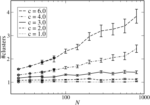
Figure 1: Average number of clusters in the solution space of the largest connected component as function of system size. The circle symbols for small system sizes have been obtained by clustering complete sets of solutions. For large systems we sampled solutions with a Monte Carlo algorithm at large but finite chemical potential $\mu$, for details see reference [34].

For every value of $N$ we sampled $10^{4}$ realizations. For each realization, we considered only the largest connected component of the given graph, since the solution-space structures of different connected components are independent of each other. The average number of clusters, as obtained from the neighborhood-based clustering using $d_{\max}=2$, as a function of the connectivity is shown as circles in figure 1. For larger system sizes, the number of cluster was estimated as described in reference [34].

For $c<e$ the number of clusters remains close to one. For larger values of $c$ the number of clusters increases with system size. Apparently the increase is compatible with a logarithmic growth as a function of system size. Hence, the change from simple to complex behavior, as expected from the analytical results [22] is visible through the cluster analysis.

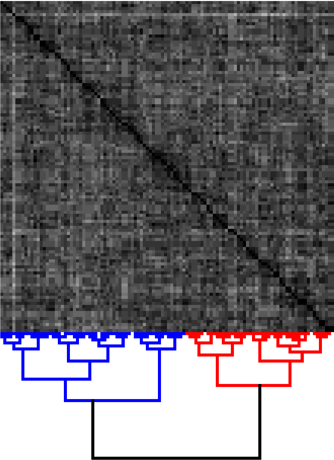
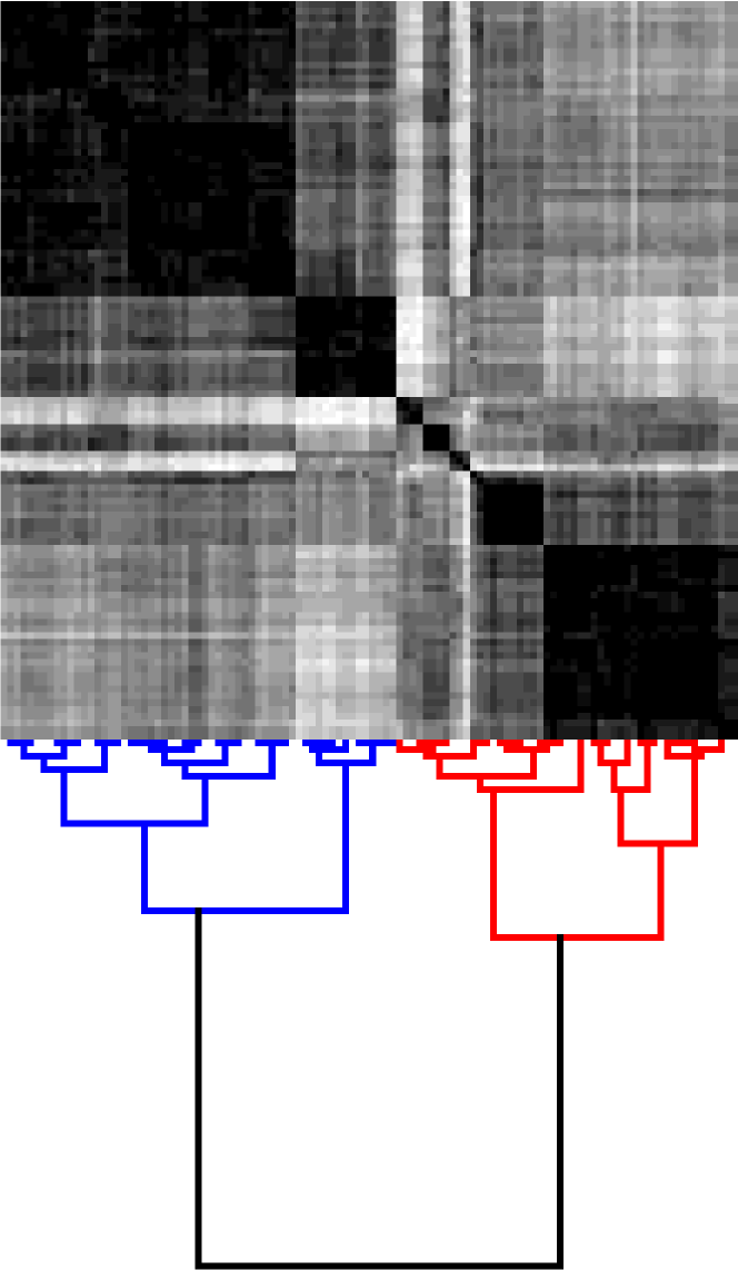
Figure 2: Sample dendrograms of 100 VC solutions for a graph with 400 vertices. Darker colors correspond to closer distances. The left one is at $c=2$, i. e. in the RS phase. There is no structure present. For $c=6$ the dendrogram provides a structure, where the solutions form clusters. The careful reader may recognize a second or third level of clustering in the right picture.

The results of the hierarchical clustering for VC are shown in figure 2. Darker colors correspond to smaller distances. The figure shows two different realizations: For small values of $c<e$, the system is in the RS phase, only a single cluster is present. For larger values of $c$, the ordering of the states obtained by the clustering algorithm reveals an underlying structure which can be seen in the right part of the figure. One can see that the states form groups where the hamming distance between the members is small (dark colors) while the distance to other states is large. Thus, our results are compatible with clustering being present for realizations with $c>e$. If you look carefully you can see more structure inside the clusters. Multiple levels of clustering indicate higher levels of RSB which we expect to be present for these values of $c$ [24, 25].

5.2 Number-partitioning problem

Next, we consider the NPP, to see whether similar clustering and coincidences can be found there as well. For all values of $k=\kappa/\kappa_{c}$ and all sizes $N$, the $Z=2\exp(0.2N)$ energetically lowest lying configurations were selected. In the solvable phase $k<1$, these are perfect partitions, while for $k>1$ we take the $Z$ configurations with the lowest values of $E$. In figure 3, the average number of clusters obtained using the neighbor-based clustering with $d_{\max}=\sqrt{N}$ is shown. In all cases, in the “easy” as well as in the “hard” phase, a basically exponential increase of the number of clusters is obtained. Note that if instead $d_{\max}=2$ had been chosen, like in the VC case, an even larger number of clusters would result, hence the large number of clusters is not an artifact of the choice of $d_{\max}$. Hence, from this result, one is tempted to conclude that the solution landscape is very complex.

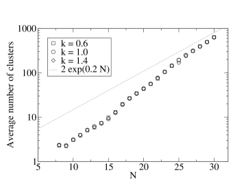
Figure 3: Average number of clusters in the solution space of the $K=2\exp(0.2N)$ energetically lowest-lying configurations as a function of the system size, for three different values of $k$. Note that $d_{\max}=\sqrt{N}$ has been used.

Nevertheless, when one performs the hierarchical clustering with a certain number (200) of randomly selected solutions ($\kappa<\kappa_{c}$) or the 200 energetically lowest lying configurations $(\kappa>\kappa_{c}$), one obtains a simple uniform distributions of the distances, without any structure visible, see figure 4. This shows, that in both regions of the phase space, the solution space basically consists of equally spaced configurations, which have a large distance from each other such that they appear as single-configuration clusters. Note that we have also studied larger systems using stochastic algorithms, and again no structure was found. Hence, the structure of the solution space is in fact simple everywhere, in contrast to the VC. This might coincide with the notion that the NPP can be seen [48] as a variant of the random-energy model [49], where each configuration is assigned a randomly and independently selected energy value.

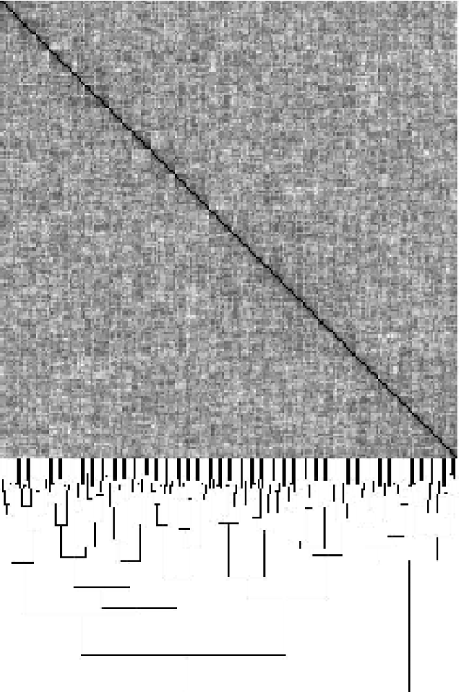
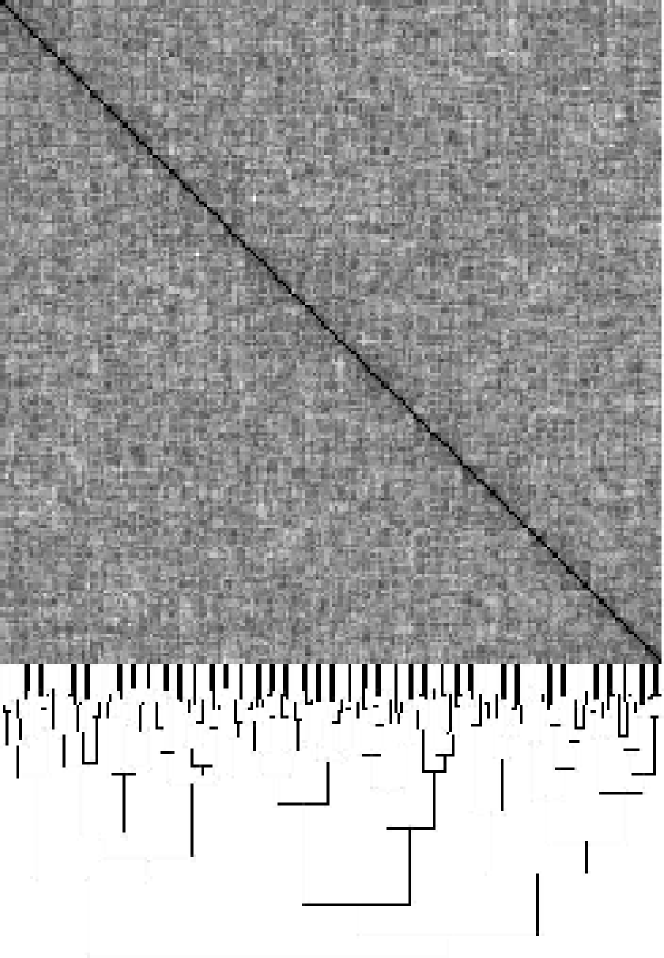
Figure 4: Sample dendrograms (bottom) and distance matrices (top) of 200 NPP solutions for systems with 35 numbers. Darker colors correspond to closer distances. The left one is at $k=1.5$, i. e. in the hard and unsolvable phase, while the right is for $k=0.6$, i.e. in the solvable phase, where perfect partitions exist. In both cases there is no structure present.

To support this finding, we have compared the solution-space structure of the NPP to a set of random bit strings (RBS), i.e. to a set of configurations with the least possible structure. For this purpose, we again use the neighborhood-based clustering with $d_{\max}=\sqrt{N}$ and measure the average number of clusters (averaged over 100 realizations) as a function of the number $Z$ of configurations included in the clustering. We do this for the NPP, for $k=1.2$, where the $Z$ energetically lowest lying configurations are considered. For the RBS case, we use $Z$ independent strings. For the RBS case, we expect that for small values of $Z$, the average number of clusters increases and is close to $Z$, because each configuration forms a single cluster. For large and even more increasing values of $Z$, the configurations are lying more dense in the configuration space, hence the number of configurations which have a neighbor within the distance $d_{\max}$ increases, leading to a decrease of the number of clusters. Finally, if $Z$ is large enough, all configurations are interconnected, hence one obtains just one single cluster. This behavior is exactly visible in figure 5. Interestingly, the resulting curves for the NPP are following very closely the curves for the RBS case, hence one can conclude that the NPP has a cluster structure which is almost indistinguishable from a random distribution, supporting the above results. Note that for VC, we find different results. The number of clusters first increases a bit, and then decreases to a value clearly above one, hence differs strongly from the RBS case.

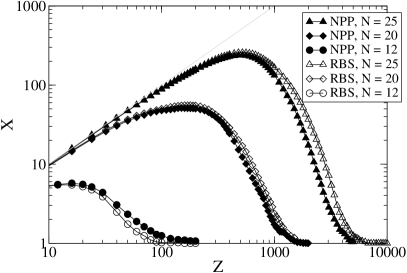
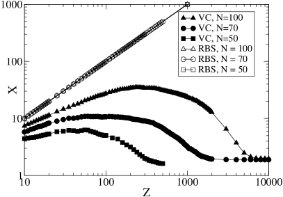
Figure 5: Average number of clusters from neighborhood-based clustering (full symbols) in the solution space of the $Z$ energetically lowest lying configurations as a function of $Z$, for different values of $N$. For comparison also the same number of clusters is shown, when instead $Z$ random bit strings are used (open symbols), i.e. the assumption of absolutely no order in the configuration space. Left: NPP for $k=1.2$, $d_{\max}=\sqrt{N}$. Right: VC for $c=4$, $d_{\max}=2$.

6 Summary and Outlook

We have studied the cluster structure of two combinatorial optimization problems, the vertex-cover problem and the number partitioning problem, on suitably defined random ensembles. In both cases, the existence of phase transitions which coincide with drastic changes of the computational complexity are analytically well established. For many of these problems, exact analytical solutions are at least currently out of reach; in particular the cluster structure of the solution landscape has been studied only very partially by analytical means. Hence, in this work, we analyze the cluster landscape numerically. We calculate exact solutions which we study using direct neighborhood clustering and via a hierarchical clustering approach. For VC, the “easy-hard” phase transition is visible also in the cluster structure of the solution space, the hard phase is dominated by a complicated hierarchy of solutions. Instead, for the NPP, the cluster structure is basically equivalent to a random distribution of the solutions in the “easy”/solvable as well as in the “hard”/unsolvable phase. Hence, a direct correspondence between the structure of the solution space, the solvability, and the hardness of finding a (best) solution does not seem to exist. Hence, the NPP seems to be hard in a different way than VC. The reason might be that the NPP is a pseudopolynomial problem, i.e. when fixing the number $M$ of bits, the problems becomes always quickly solvable for $N\to\infty$ .

To further elucidate possible relationships, other optimization problems should be studied in this way in the future. In particular the authors are currently working on the satisfiability problem, where several changes of the solution-space structure are expected from approximate analytical solutions [16, 30].

7 Acknowledgments

The authors have received financial support from the VolkswagenStiftung (Germany) within the program “Nachwuchsgruppen an Universitäten”, and from the European Community via the DYGLAGEMEM program.

References

- [1] Garey M R and Johnson D S 1979 Computers and intractability (San Francisco: W.H. Freemann)
- [2] Binder K and Young A 1986 Rev. Mod. Phys. 58 801
- [3] Mézard M, Parisi G and Virasoro M 1987 Spin glass theory and beyond (Singapore: World Scientific)
- [4] Fischer K and Hertz J 1991 Spin Glasses (Cambridge: Cambridge University Press)
- [5] Young A P (ed) 1998 Spin glasses and random fields (Singapore: World Scientific)
- [6] Sherrington D and Kirkpatrick S 1975 Phys. Rev. Lett. 35 1792
- [7] Parisi G 1979 Phys. Rev. Lett. 43 1754
- [8] Parisi G 1983 Phys. Rev. Lett. 50 1946
- [9] Rammal R, Toulouse G and Virasoro M A 1986 Rev. Mod. Phys. 58 765
- [10] Young A P 1983 Phys. Rev. Lett. 51 13
- [11] Parisi G, Ritort F and Slanina F 1993 J. Phys. A 26 3775
- [12] Billoire A, Franz S and Marinari E 2003 J. Phys. A 36 15
- [13] Sinova J, Canright G and MacDonald A H 2000 Phys. Rev. Lett. 85 2609
- [14] Sinova J, Canright G, Castillo H and MacDonald A H 2001 Phys. Rev. B 63 104427
- [15] Hed G, Young A P and Domany E 2004 Phys. Rev. Lett. 92 157201
- [16] Biroli G, Monasson R and Weigt M 2000 Eur. Phys. J. B 14 551
- [17] Mézard M, Parisi G and Zecchina R 2002 Science 297 812
- [18] Mézard M and Zecchina R 2002 Phys. Rev. E 66 056126
- [19] Mertens S 1998 Phys. Rev. Lett. 81 4281
- [20] Mertens S 2000 Phys. Rev. Lett. 84 1347
- [21] Mulet R, Pagnani A, Weigt M and Zecchina R 2002 Phys. Rev. Lett. 89 268701
- [22] Weigt M and Hartmann A K 2000 Phys. Rev. Lett. 84 6118
- [23] Hartmann A K and Weigt M 2001 Theor. Comp. Sci. 265 199
- [24] Weigt M and Hartmann A K 2001 Phys. Rev. E 63 056127
- [25] Zhou H 2003 Eur. Phys. J. B 32 265
- [26] Hartmann A K and Weigt M 2003 J. Phys. A 36 11069
- [27] Monasson R and Zecchina R 1996 Phys. Rev. Lett. 76 3881
- [28] Monasson R, Zecchina R, Kirkpatrick S, Selman B and Troyansky L 1999 Nature 400 133
- [29] Weigt M 2004 New Optimization Algorithms in Physics ed Hartmann A K and Rieger H (Weinheim: Wiley-VCH)
- [30] Zecchina R 2004 New Optimization Algorithms in Physics ed Hartmann A K and Rieger H (Weinheim: Wiley-VCH)
- [31] Mézard M, Ricci-Tersenghi F and Zecchina R 2003 J. Stat. Phys. 111 505
- [32] Bauer M and Golinelli O 2001 Eur. Phys. J. B 24 339
- [33] Bauer M and Golinelli O 2001 Phys. Rev. Lett. 86 2621
- [34] Barthel W and Hartmann A K 2004 Phys. Rev. E 70 066120
- [35] Hartmann A K and Rieger H 2001 Optimization Algorithms in Physics (Weinheim: Wiley-VCH)
- [36] Gent I P and Walsh T 1996 Proceedings of 12th European Conference on Artificial Intelligence. ECAI ’96 (Chichester: Wiley) p 170
- [37] Borgs C, Chayes J and Pittel B 2001 Rand. Struct. Alg. 19 247
- [38] Korf R E 1998 Artif. Intell. 106 181
- [39] Lawler E L and Wood D E 1966 Oper. Res. 14 699
- [40] Hartmann A K and Weigt M 2005 Phase Transitions in Combinatorial Optimization Problems (Weinheim: Wiley-VCH)
- [41] Tarjan R E and Trojanowski A E 1977 SIAM J. Comp. 6 537
- [42] Mertens S 2006 Computational Complexity and Statistical Physics ed Percus A G, Istrate G and Moore C (New York: Oxford University Press) p 125
- [43] Hartmann A K 2001 Phys. Rev. E 63 016106
- [44] Jain A K and Dubes R C 1988 Algorithms for Clustering Data (Englewood Cliffs, USA: Prentice-Hall)
- [45] Hed G, Hartmann A K, Stauffer D and Domany E 2001 Phys. Rev. Lett. 86 3148
- [46] Ciliberti S and Marinari E 2004 J. Stat. Phys. 115 557
- [47] Ward J 1963 J. of the Am. Stat. Association 58 236
- [48] Bauke H, Franz S and Mertens S 2004 JSTAT 4 P04003
- [49] Derrida B 1991 Phys. Rev. B 24 2613