Residual Coulomb interaction fluctuations in chaotic systems: the boundary, random plane waves, and semiclassical theory

Abstract

New fluctuation properties arise in problems where both spatial integration and energy summation are necessary ingredients. The quintessential example is given by the short-range approximation to the first order ground state contribution of the residual Coulomb interaction. The dominant features come from the region near the boundary where there is an interplay between Friedel oscillations and fluctuations in the eigenstates. Quite naturally, the fluctuation scale is significantly enhanced for Neumann boundary conditions as compared to Dirichlet. Elements missing from random plane wave modeling of chaotic eigenstates lead surprisingly to significant errors, which can be corrected within a purely semiclassical approach.

The characterization of quantum systems with any of a variety of underlying classical dynamics, ranging from diffusive to chaotic to regular, has often demonstrated that the study of their statistical properties is of primary importance. Spectral fluctuations are a principle example as they gave the first support to one of the main results linking classical chaos and random matrix theory Mehta (2004), the Bohigas-Giannoni-Schmit conjecture Bohigas et al. (1984); Bohigas (1991). Needless to say, the statistical properties of eigenfunctions are also a subject of paramount interest Berry (1977); Voros (1979); McDonald and Kaufman (1979); McDonald (1983); Heller (1984, 1991); Srednicki (1996); Hortikar and Srednicki (1998); Mirlin (2000).

For chaotic systems, a widely accepted starting point for the treatment of eigenfunction fluctuations locally, such as the amplitude distribution or the two-point correlation function $c(|{\bf r}-{\bf r}^{\prime}|)=\langle\psi({\bf r})\psi({\bf r}^{\prime})\rangle$ of a given eigenfunction $\psi$, is a modeling in terms of a random superposition of plane waves (RPW) Berry (1977); Voros (1979). For two-degree-of-freedom systems, $c(r)$ can be understood as being given approximately by a Bessel function. For distances $|{\bf r}-{\bf r}^{\prime}|$ short compared to the system size, and in the absence of effects related to classical dynamics Heller (1984, 1991); Bohigas et al. (1993), this is roughly observed in numerical McDonald (1983); McDonald and Kaufman (1988); Bäcker and Schubert (2002) and experimental Kim et al. (2003) studies. Our interest here is in statistical properties of eigenfunctions going beyond local quantities such as $c(r)$.

One motivation for the introduction of these new statistical measures is to study the interplay between interferences and interactions in mesoscopic systems. For typical electronic densities, the screening length is close to the Fermi wavelength $\lambda_{\scriptscriptstyle F}$, and the screened Coulomb interaction can be approximated by the short range expression $V_{\rm sc}({\bf r}-{\bf r}^{\prime})=({2\nu})^{-1}{F_{0}^{a}}\delta({\bf r}-{\bf r}^{\prime})$ with $2\nu$ the mean local density of states, including spin degeneracy, ($\nu\!=\!m/2\pi\hbar^{2}$ for $d\!=\!2$) and $F_{0}^{a}$ the dimensionless Fermi liquid parameter Pines and Nozières (1966), a constant of order one.

To this level of approximation, the first order ground state energy contribution of the residual interactions can be expressed in the form $\delta E^{\rm RI}=(2\nu)^{-1}{F_{0}^{a}}\int d{\bf r}\,N_{\uparrow}({\bf r})N_{\downarrow}({\bf r}),$ with $N_{\sigma}$ the unperturbed ground state density of particles with spin $\sigma$. From this expression, it is seen that the increase of interaction energy associated with the addition of an extra electron is related to

$${{\cal S}_{i}}={\cal A}\int{\rm d}{\bf r}\ \left|\Psi_{i}({\bf r})\right|^{2}N({\bf r};E_{i}^{+})\;,$$ (1)

with $N({\bf r};E)\equiv\sum_{i=1}^{\infty}\left|\Psi_{i}({\bf r})\right|^{2}\theta\left(E-E_{i}\right)$ and the understanding that $E_{i}<E_{i}^{+}<E_{i+1}$. Our goal in this letter is to study the fluctuation properties of the ${{\cal S}_{i}}$, concentrating on the case of two dimensional billiards with either Dirichlet or Neumann boundary conditions. For them, $\cal A$ is the billiard area.

The dominant contributions to ${\cal S}_{i}$ (and its fluctuations) originate from the Friedel oscillations of the density of particles near the boundary. For billiards systems, they can be expressed as $N_{\rm Friedel}({\bf r};E)=\frac{N_{W}(E)}{{\cal A}}\left[1\pm\frac{J_{1}(2kx)}{kx}\right]$ Bäcker et al. (1998), with $x$ the distance from the boundary, the $+$ and $-$ sign corresponding respectively to Neumann and Dirichlet boundary conditions, and $N_{W}(E)$ refers to leading term of the Weyl formula, $N_{W}(E)=\nu{\cal A}E$. To leading order we can therefore use the approximation

$${\cal S}_{i}=i\pm i\int{\rm d}{\bf r}\ \left[\frac{J_{1}(2k_{\scriptscriptstyle F}x)}{k_{\scriptscriptstyle F}x}|\Psi_{i}({\bf r})|^{2}\right]\;.$$ (2)

To proceed, a description of the fluctuations of $\left|\Psi_{i}({\bf r})\right|^{2}$ is also required. These are obtained ahead using a semiclassical approach closely related to the Gutzwiller trace formula. However, it is useful first to consider the oft-employed RPW description, which very interestingly turns out to lack a couple of crucial ingredients. Nevertheless, it sheds light on the mechanism governing the fluctuations under study.

Within RPW Berry (1977); Voros (1979) eigenstates are represented, in the absence of any symmetry, by a random superposition of plane waves $\sum_{l}a_{l}\exp(i{\bf k}_{l}\cdot{\bf r})$ with wave-vectors of fixed modulus $|{\bf k}_{l}|=k_{\scriptscriptstyle F}$ distributed isotropically. Time reversal invariance introduces a correlation between time reversed plane waves such that the eigenfunctions are real. Similarly, the presence of a planar boundary imposes a constraint between the coefficients of plane waves related by a sign change of the normal component of the wave-vector ${\bf k}_{l}$ Berry (2002); Urbina and Richter (2004). Near a boundary, and using a system of coordinates ${\bf r}=\hat{\bf x}+\hat{\bf y}$ with ($\hat{\bf x}$,$\hat{\bf y}$) the vectors respectively parallel and perpendicular to the boundary, eigenfunctions are mimicked statistically by a superposition,

$$\psi_{i}({\bf r})=\frac{1}{N_{\rm eff}}\sum_{l=1}^{N_{\rm eff}}a_{l}{\bf cs}\left({\bf k}_{l}\cdot\hat{\bf x}\right)\cos\left({\bf k}_{l}\cdot\hat{\bf y}+\varphi_{l}\right)$$ (3)

where ${\bf cs}(\cdot)\stackrel{{\scriptstyle\rm def}}{{=}}\sin(\cdot)$ for Dirichlet and $\cos(\cdot)$ for Neumann boundary conditions. The phase angle $\varphi_{l}$, the orientation of the wave vector ${\bf k}_{l}$, and the real amplitude $a_{l}$ with $\langle a_{l}a_{l^{\prime}}\rangle=\delta_{l{l^{\prime}}}\sigma^{2}$ are all chosen randomly. Normalization of the wave-functions fixes the variance $\sigma^{2}$ through the relation

$$1=\int d{\bf r}\,\left<\left|\psi_{i}({\bf r})\right|^{2}\right>=\frac{{\cal A}\sigma^{2}}{4N_{\rm eff}}\left(1\pm\frac{{\cal L}}{2k_{\scriptscriptstyle F}{\cal A}}\right)\;,$$ (4)

where $\cal L$ is the perimeter.

The variance is a natural measure of the fluctuations. To leading order

$$\begin{split}{\rm Var}&\left({\cal S}_{i}\right)=\frac{i^{2}}{{\cal A}^{2}}\int{\rm d}{\bf r}_{1}{\rm d}{\bf r}_{2}\ \frac{J_{1}(2k_{\scriptscriptstyle F}x_{1})}{k_{\scriptscriptstyle F}x_{1}}\frac{J_{1}(2k_{\scriptscriptstyle F}x_{2})}{k_{\scriptscriptstyle F}x_{2}}\\ \times&\left[\left<|\Psi_{i}({\bf r}_{1})|^{2}|\Psi_{i}({\bf r}_{2})|^{2}\right>-\left<|\Psi_{i}({\bf r}_{1})|^{2}\right>\left<|\Psi_{i}({\bf r}_{2})|^{2}\right>\right]\;.\end{split}$$

The fluctuations are thus given by pair-wise correlating the random plane wave coefficients $a_{n}$ such that $\langle a_{l}a_{l^{\prime}}a_{m}a_{m^{\prime}}\rangle=\langle a_{l}a_{l^{\prime}}\rangle\langle a_{m}a_{m^{\prime}}\rangle+\langle a_{l}a_{m}\rangle\langle a_{l^{\prime}}a_{m^{\prime}}\rangle+\langle a_{l}a_{m^{\prime}}\rangle\langle a_{l^{\prime}}a_{m}\rangle=\sigma^{4}\left(\delta_{ll^{\prime}}\delta_{mm^{\prime}}+\delta_{lm}\delta_{l^{\prime}m^{\prime}}+\delta_{lm^{\prime}}\delta_{l^{\prime}m}\right)$. One obtains in this way

$$\begin{split}{\rm Var}&\left[{\cal S}_{i}\right]=\frac{8i^{2}}{{\cal A}^{2}}\frac{1}{N_{\rm eff}^{2}}\sum^{N_{\rm eff}}_{l,m=1}\int d{\bf r}_{1}d{\bf r}_{2}\frac{J_{1}(2k_{\scriptscriptstyle F}x_{1})}{k_{\scriptscriptstyle F}x_{1}}\frac{J_{1}(2k_{\scriptscriptstyle F}x_{2})}{k_{\scriptscriptstyle F}x_{2}}\\ &{\bf cs}({\bf k}_{l}\cdot{\bf x}_{1}){\bf cs}({\bf k}_{l}\cdot{\bf x}_{2}){\bf cs}({\bf k}_{m}\cdot{\bf x}_{1}){\bf cs}({\bf k}_{m}\cdot{\bf x}_{2})\\ &\cos\left[{\bf k}_{l}\cdot({\bf y}_{1}-{\bf y}_{2})\right]\cos\left[{\bf k}_{m}\cdot({\bf y}_{1}-{\bf y}_{2})\right]\;.\end{split}$$ (5)

Performing the integral gives

$${\rm Var}[{\cal S}_{i}]=\frac{k_{\scriptscriptstyle F}{\cal L}}{4\pi^{3}}\langle\lambda^{2}(\theta)\rangle_{\theta}$$ (6)

where we have introduced the function $\lambda(\theta)\stackrel{{\scriptstyle\rm def}}{{=}}\left[{1\pm|\sin(\bar{\theta})|}\right]/|\cos(\bar{\theta})|$ and the expression for $\langle\lambda^{2}(\theta)\rangle_{\theta}\equiv\int_{0}^{1}d(\sin\theta)\lambda^{2}(\theta)$ is given ahead in Eq. (15).

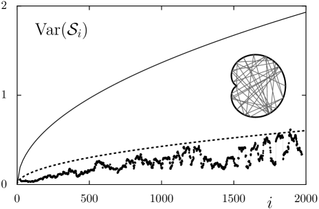
Figure 1: Variance of ${\cal S}_{i}$ for the cardioid billiard with Dirichlet boundary conditions. The solid line is the RPW expression, Eq. (6), the dashed line is the semiclassical prediction, Eq. (14), and the discrete points are for the cardioid billiard (shown in inset).

In Fig. 1, the variance of ${{\cal S}_{i}}$ as a function of $i$ is represented for a chaotic system, the cardioid billiard with Dirichlet boundary conditions Robnik (1984); Bäcker et al. (1995). In this case, quite surprisingly given the history of modeling chaotic eigenstates within the RPW framework, its predictions significantly overestimate the fluctuations. In fact, two important elements are missing from this approach, both of which are addressed properly within a purely semiclassical approach.

One difficulty immediately encountered with a semiclassical treatment of the ${{\cal S}_{i}}$ is that their computation implies addressing the fluctuations of individual wave-functions, whereas the semiclassical approximations valid for chaotic systems of use here converge only for (locally) smoothed quantities. This difficulty may be overcome by following the spirit of Bogomolny’s calculation Bogomolny (1988), and introducing a local energy averaging,

$$\langle{\cal S}\rangle_{\Delta N}\stackrel{{\scriptstyle\rm def}}{{=}}\frac{1}{\Delta N}\sum_{E-\frac{\Delta E}{2}<E_{i}<E+\frac{\Delta E}{2}}{{\cal S}_{i}}\;,$$ (7)

with $\Delta N\stackrel{{\scriptstyle\rm def}}{{=}}N(E\!+\!\frac{\Delta E}{2})\!-\!N(E\!-\!\frac{\Delta E}{2})$. This generates the relation

$${\rm Var}[\langle{\cal S}\rangle_{\Delta N}]\stackrel{{\scriptstyle\rm def}}{{=}}\overline{\left({\langle{\cal S}\rangle_{\Delta N}}-\overline{\cal S}\right)^{2}}$$ (8)

$$= \frac{1}{\Delta N}{{\rm Var}[{\cal S}_{i}]}+\left(1-\frac{1}{\Delta N}\right){\rm Covar}\left[{\cal S}_{i}{\cal S}_{i+j}\right].$$

assuming that there is translational invariance (smooth, uniform behavior) locally in indices ($i,j$). See Ullmo et al. for further discussion for the relevance of this assumption. Computing the smoothed quantity ${\langle{\cal S}\rangle_{\Delta N}}$, for which semiclassical approximations are convergent, one can therefore extract the variance of the ${{\cal S}_{i}}$ from the scaling in $\Delta N$ of ${\rm Var}[\langle{\cal S}\rangle_{\Delta N}]$.

Our starting point for this calculation is

$${\cal A}\langle|\Psi_{i}({\bf r})|^{2}\rangle_{\Delta N} = 1\pm J_{0}(2k_{\scriptscriptstyle F}x)-\frac{1}{\nu}\frac{1}{\pi}{\rm Im}\langle\tilde{G}^{\rm osc}({\bf r},{\bf r},E)\rangle_{\Delta E}$$ (9)

$$-\frac{1\pm J_{0}(2k_{\scriptscriptstyle F}x)}{{\cal A}\nu}\langle\rho^{\rm osc}\rangle_{\Delta E}\;,$$

valid near the boundary, which differs from the expression given by Bogomolny Bogomolny (1988) only through the inclusion of the Bessel function $J_{0}(2k_{\scriptscriptstyle F}x)$ accounting for the Friedel oscillations. Here, the energy smoothing indicated is similar to above except normalized by the energy range, and $\rho^{\rm osc}$ is the oscillating part of the density of states, given semiclassically as a sum over periodic orbits

$$\rho^{\rm osc}(E)=\frac{1}{\pi\hbar}\sum_{\gamma={\rm p.\,o.}}\tau_{\gamma}\frac{\cos\left(\frac{S_{\gamma}(E^{+}_{i})}{\hbar}-\sigma_{\gamma}\frac{\pi}{2}\right)}{\left|\operatorname{Det}\left(M_{\gamma}-{\bf 1}\right)\right|^{1/2}}\;.$$ (10)

Similarly, the diagonal part of the Green’s function $G^{R}({\bf r},{\bf r},E)$ is expressed as a sum over closed (not necessarily periodic) orbits

$$\begin{split}G^{\rm osc}({\bf r},{\bf r},E)&\simeq\frac{1}{i\hbar}\frac{1}{\sqrt{2i\pi\hbar}}\sum_{\mu:{\bf r}\to{\bf r}}\frac{1}{\sqrt{|\dot{x}\dot{x}^{\prime}m_{12,\mu}|}}\\ &\times\exp\left[\frac{i}{\hbar}S_{\mu}({\bf r},{\bf r},E)-i\frac{\pi}{2}\eta_{\mu}\right]\;.\end{split}$$ (11)

In the above expressions, $S$ is the action integral along the orbit, $\tau$ the period, $m_{12}\equiv\partial y^{\rm final}/\partial p_{y}^{\rm initial}$, $M_{\gamma}$ the monodromy matrix, and $\sigma_{\gamma}$, $\eta_{\mu}$ are Maslov indices. The tilde on the Green’s function in Eq. (9) furthermore indicates that the short orbit giving rise to Friedel oscillations, namely the one bouncing off the boundary and returning directly to its initial location, is excluded from the semiclassical sum (as in Eq. (9) it is already taken into account by the Bessel function).

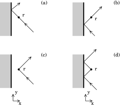
Figure 2: In the semiclassical sums, the four orbits which, as $x\to 0$, coalesce into the same [nearly] periodic orbit, need to be aggregated. The top row correspond to two (nearly) periodic orbits. The bottom row correspond to two non periodic orbits ($p^{\prime}_{x}=-p_{x})$.

Inserting Eq. (9) into Eq. (2), and performing the integral over space, it is important to note that the range of integration in the direction perpendicular to the boundary is short, even on the quantum scale, and that therefore a stationary phase condition should be imposed only on the parallel direction. Gathering however the four orbits shown in Fig 2, and labelling their total contribution with the index $\gamma$ of the periodic orbit to which they converge as $x\to 0$, one obtains, following the usual steps of the derivation of the Gutzwiller trace formula,

$$\langle{\cal S}\rangle_{\Delta N}-\overline{\cal S} =\pm\frac{1}{\pi}\sum_{\gamma={\rm p.\,o.}}\frac{\cos\left[\frac{S_{\gamma}(E)}{\hbar}-\bar{\nu}_{\gamma}\frac{\pi}{2}\right]}{\sqrt{|\operatorname{Det}(M_{\gamma}-1)|}}\times$$ (12)

$${\rm sinc}\left(\frac{\tau_{\gamma}\Delta E}{2\hbar}\right)\sum_{l\in\gamma}\left(\lambda(\theta_{l})-\tilde{\lambda}_{\gamma}\right),$$

where $\lambda(\theta_{l})$ is the function introduced in Eq. (6) evaluated at the angle at which the periodic orbit $\gamma$ strikes the boundary on the $l^{th}$ bounce, and $\tilde{\lambda}_{\gamma}\stackrel{{\scriptstyle\rm def}}{{=}}\frac{{\cal L}\ell_{\gamma}}{2{\cal A}n_{\gamma}}\left(1\pm\frac{2}{\pi}\right)$, with $\ell_{\gamma}$ the total length and $n_{\gamma}$ the number of bounces of the orbit $\gamma$.

Eq. (12) can be used directly to compute the Fourier transform of the ${{\cal S}_{i}}$, yielding a structure very similar to that of the density of states Eq. (10). Both Fourier transforms can be done so as to have peaks with the same shape and positions, but different amplitudes. Eq. (12) can be furthermore used to compute the variance of $\langle{\cal S}\rangle_{\Delta N}$. To begin, square Eq. (10), use the diagonal approximation in which orbits are paired only with themselves or their time reverse symmetric partner, and apply the Hannay Ozorio de Almeida sum rule Ozorio de Almeida (1988)

$$\sum_{\gamma={\rm p.o.}}\frac{n}{|\operatorname{Det}(M_{l}-1)|}=1\;,$$

where only periodic orbits of $n$ bounces from the boundary are included. Then for the long orbits relevant here, replace the mean length $\ell_{\gamma}/n_{\gamma}$ between two successive bounces for a specific orbit $\gamma$ by $\bar{d}={\pi{\cal A}}/{\cal L}$, the mean length between bounces averaged for all initial conditions on the boundary. Noting $\left\langle\lambda(\theta)-\tilde{\lambda}\right\rangle=0$, this gives

$$\overline{\left(\langle{\cal S}\rangle_{\Delta N}-\overline{\cal S}\right)^{2}}=\frac{k_{\scriptscriptstyle F}{\cal L}}{2\pi^{3}}\left\langle\left(\lambda(\theta)-\tilde{\lambda}\right)^{2}\right\rangle_{\theta}\,\frac{1}{\Delta N}\;.$$ (13)

As before, angle average $\langle\cdot\rangle_{\theta}$ is over the measure $d\sin\theta$.

The structure of this result is quite interesting. The surviving contribution comes from what may be called the “diagonal-diagonal” terms, i.e. pairing not only of the same orbit but of the same bounce from the boundary. This term contributes only to the variance as it scales as $1/\Delta N$; see Eq. (8). The terms that would be called “diagonal-off-diagonal” give a vanishing contribution. In addition, note the absence of a constant term. It implies that the covariance vanishes, which is consistent with our cardioid billiard calculations (not shown here).

Thus, from Eq. (8) and the above considerations

$$\mbox{Var}({\cal S}_{i})=\frac{k_{\scriptscriptstyle F}{\cal L}}{2\pi^{3}}\times\left\langle\left(\lambda(\theta)-\langle\lambda\right\rangle_{\theta}\right)^{2}\rangle_{\theta}$$ (14)

where

$$\begin{split}&\left\langle\left(\lambda(\theta)-\langle\lambda\right\rangle_{\theta}\right)^{2}\rangle_{\theta}\\ &=\left\{\begin{array}[]{ll}(2\ln 2-1)-\left(\frac{\pi}{2}-1\right)^{2}\simeq 0.06&\mbox{Dirichlet }\\ (2\ln 2-1)-\left(\frac{\pi}{2}-1\right)^{2}+4\left(\ln\frac{\pi k_{\scriptscriptstyle F}{\cal A}}{2{\cal L}}-\frac{\pi}{2}\right)&\mbox{Neumann}\end{array}\right.\end{split}$$ (15)

Comparing this expression with Eq. (6), we see that the semiclassical approach and the random plane wave model lead to the same result, except for two differences. First, a factor two in the prefactor can be traced to dynamical correlations missed by RPW. The nature of these correlations, which are somewhat subtle, will be discussed in Ullmo et al. . Second, the mean square $\langle\lambda^{2}(\theta)\rangle_{\theta}$ has been replaced by the variance of $\lambda(\theta)$, giving now a much better agreement with the numerically evaluated ${\cal S}_{i}$ (see Fig. 1).

In Eq. (12), the term proportional to $\lambda(\theta_{\gamma})$ can be seen to arise from $G^{\rm osc}$ in Eq. (9), while the one proportional to $\tilde{\lambda}_{\gamma}$ originates from $\rho^{\rm osc}$. The random plane wave result is thus, in some sense, ignoring the latter contribution. As $\rho^{\rm osc}$ has no spatial dependence, its role is not to describe the variations of the wave-function, but rather to ensure their normalization (as can be seen readily by integrating Eq. (9) over space). Therefore the main reason of the failure of the RPW approach is due to the lack of individually normalized wavefunctions, and more precisely to the fact that Eq. (4) imposes the normalization of the wavefunctions only on average Urbina and Richter (2007).

Equation (14) emphasizes the importance of the boundary conditions. Indeed, the variance of $\lambda(\theta)$ is extremely small for Dirichlet boundary conditions, which has to be expected since the wave-functions are zero near the boundary. As a consequence, and as seen in Fig. 1, the fluctuations remain smaller than one even for a relatively large number of particles, in spite of the linear $(k_{\scriptscriptstyle F}{\cal L})$ dependence of the variance. On the other hand, Neumann boundary conditions yield a logarithmic divergence which can be considered in practice as a constant somewhat larger than one. Fluctuations in this case are greatly enhanced with respect to the Dirichlet case.

To conclude, “integrated” wavefunction statistics are introduced, in part motivated by the need to understand the effect of interactions on ground state properties in quantum dots. A significant part of their fluctuation properties can be understood with basic RPW modeling. However, a semiclassical framework is developed here, which indicates missing ingredients of RPW, and in particular that lack of individual state normalization leads to a significant overestimate of the fluctuations. It turns out furthermore that boundary conditions, which are often not discussed in the context of mesoscopic systems, play an important role.

We stress finally that only the extreme limit of strongly chaotic systems has been treated here. For less developed chaos, or systems with some regular dynamics, where some eigenstate localization exists, there may be significant enhancements in the fluctuations and correspondingly greater effects on ground state properties Ullmo et al. (2003). The consequences for experimentally realizable systems and for such systems with some form of eigenstate localization is left for future study.

One of us (ST) gratefully acknowledges support from US National Science Foundation grant PHY-0555301.

References

- Mehta (2004) M. L. Mehta, Random Matrices (Third Edition) (Elsevier, Amsterdam, 2004).
- Bohigas et al. (1984) O. Bohigas, M. J. Giannoni, and C. Schmit, Phys. Rev. Lett. 52, 1 (1984).
- Bohigas (1991) O. Bohigas, in Chaos and Quantum Physics, edited by M. J. Giannoni, A. Voros, and J. Jinn-Justin (North-Holland, Amsterdam, 1991), pp. 87–199.
- Berry (1977) M. V. Berry, J. Phys. A 10, 2083 (1977).
- Voros (1979) A. Voros, in Stochastic Behaviour in Classical and Quantum Hamiltonian Systems, edited by G. Casati and G. Ford (Springer-Verlag, Berlin, 1979), p. 334.
- McDonald and Kaufman (1979) S. W. McDonald and A. N. Kaufman, Phys. Rev. Lett. 42, 1189 (1979).
- McDonald (1983) S. W. McDonald, Ph.D. thesis, University of California, Lawrence Berkeley Laboratory (1983), [Report No. LBL-14837].
- Heller (1984) E. J. Heller, Phys. Rev. Lett. 53, 1515 (1984).
- Heller (1991) R. Heller, in Chaos and Quantum Physics, edited by M. J. Giannoni, A. Voros, and J. Jinn-Justin (North-Holland, Amsterdam, 1991).
- Srednicki (1996) M. Srednicki, Phys. Rev. E 54, 954 (1996).
- Hortikar and Srednicki (1998) S. Hortikar and M. Srednicki, Phys. Rev. Lett. 80, 1646 (1998).
- Mirlin (2000) A. D. Mirlin, Phys. Rep. 326, 259 (2000).
- Bohigas et al. (1993) O. Bohigas, S. Tomsovic, and D. Ullmo, Phys. Rep. 223, 43 (1993).
- McDonald and Kaufman (1988) S. W. McDonald and A. N. Kaufman, Phys. Rev. A 37, 3067 (1988).
- Bäcker and Schubert (2002) A. Bäcker and R. Schubert, J. Phys. A: Math. Gen. 35, 539 (2002).
- Kim et al. (2003) Y.-H. Kim, M. Barth, U. Kuhl, and H.-J. Stöckmann, Prog. Theor. Phys. Suppl. 150, 105 (2003).
- Pines and Nozières (1966) D. Pines and P. Nozières, Theory of Quantum Liquids Vol. I. (W. A. Benjamin, New York, 1966).
- Bäcker et al. (1998) A. Bäcker, R. Schubert, and P. Stifter, Phys. Rev. E 57, 5425 (1998), erratum ibid. 58, 5192 (1998).
- Berry (2002) M. V. Berry, J. Phys. A 35, 3025 (2002).
- Urbina and Richter (2004) J. D. Urbina and K. Richter, Phys. Rev. E 70, 015201 (2004).
- Robnik (1984) M. Robnik, J. Phys. A: Math. Gen. 17, 1049 (1984).
- Bäcker et al. (1995) A. Bäcker, F. Steiner, and P. Stifter, Phys. Rev. E 52, 2463 (1995).
- Bogomolny (1988) E. Bogomolny, Physica D 31, 169 (1988).
- (24) D. Ullmo, S. Tomsovic, and A. Bäcker, in preparation.
- Ozorio de Almeida (1988) A. M. Ozorio de Almeida, Hamiltonian systems: Chaos and quantization (Cambridge University Press, Cambridge, 1988).
- Urbina and Richter (2007) J. D. Urbina and K. Richter, Eur. Phys. J. ST 145, 255 (2007).
- Ullmo et al. (2003) D. Ullmo, T. Nagano, and S. Tomsovic, Phys. Rev. Lett. 90, 176801 (2003).