Mass, Metal, and Energy Feedback in Cosmological Simulations

Abstract

Using Gadget-2 cosmological hydrodynamic simulations including an observationally-constrained model for galactic outflows, we investigate how feedback from star formation distributes mass, metals, and energy on cosmic scales from $z=6\rightarrow 0$. We include instantaneous enrichment from Type II supernovae (SNe), as well as delayed enrichment from Type Ia SNe and stellar (AGB) mass loss, and we individually track carbon, oxygen, silicon, and iron using the latest yields. Following on the successes of the momentum-driven wind scalings (e.g. Oppenheimer & Davé 2006), we improve our implementation by using an on-the-fly galaxy finder to derive wind properties based on host galaxy masses. By tracking wind particles in a suite of simulations, we find: (1) Wind material reaccretes onto a galaxy (usually the same one it left) on a recycling timescale that varies inversely with galaxy mass (e.g. $<1$ Gyr for $L^{*}$ galaxies at $z=0$). Hence metals driven into the IGM by galactic superwinds cannot be assumed to leave their galaxy forever. Wind material is typically recycled several times; the median number of ejections for a given wind particle is 3, so by $z=0$ the total mass ejected in winds exceeds $0.5\Omega_{b}$. (2) The physical distance winds travel is fairly independent of redshift and galaxy mass ($\sim 60-100$ physical kpc, with a mild increase to lower masses and redshifts). For sizable galaxies at later epochs, winds typically do not escape the galaxy halo, and rain back down in a halo fountain. High-$z$ galaxies enrich a significantly larger comoving volume of the IGM, with metals migrating back into galaxies to lower $z$. (3) The stellar mass of the typical galaxy responsible for every form of feedback (mass, metal, & energy) grows by $\sim 30\times$ between $z=6\rightarrow 2$, but only $\sim 2-3\times$ between $z=2\rightarrow 0$, and is around or below $L^{*}$ at all epochs. (4) The energy imparted into winds scales with $M_{\rm gal}^{1/3}$, and is roughly near the supernova energy. Given radiative losses, energy from another source (such as photons from young stars) may be required to distribute cosmic metals as observed. (5) The production of all four metals tracked is globally dominated by Type II SNe at all epochs. However, intracluster gas iron content triples as a result of non-Type II sources, and the low-$z$ IGM carbon content is boosted significantly by AGB feedback. This is mostly because gas is returned into the ISM to form one-third more stars by $z=0$, appreciably enhancing cosmic star formation at $z\la 1$.

1 Introduction

Galactic-scale feedback appears to play a central role in the evolution of galaxies and the intergalactic medium (IGM) over the history of the Universe. Mass feedback in the form of galactic outflows curtails star formation (e.g. , 2003b, hereafter SH03b) by removing baryons from sites of star formation, thereby solving the overcooling problem where too many baryons condense into stars (e.g. , 2001). The energy in these winds carry metal-enriched galactic interstellar medium (ISM) gas out to large distances, where the metals are observed in quasar-absorption line spectra tracing the IGM (e.g. , 1998). Galactic outflows appear to be the only viable method to enrich the IGM to the observed levels as simulations show that tidal stripping only is not sufficient (, 2001, 2006, hereafter OD06). Hence understanding galactic outflows is a key requirement for developing a complete picture of how baryons in all cosmic phases evolve over time.

Modeling galactic outflows in a cosmological context has now become possible thanks to increasingly sophisticated algorithms and improving computational power. The detailed physics in distributing the feedback energy from supernovae and massive stars to surrounding gas still remains far below the resolution limit in such simulations, so must be incorporated heuristically. There are two varieties of approaches of feedback: thermal and kinetic. (2004) injects energy from galactic superwinds and supernovae thermally into a number of surrounding gas particles in a Smoothed Particle Hydrodynamic (SPH) simulation, and find that hypernovae with 10$\times$ the typical supernova energy are needed to enrich the IGM to observed levels while matching the stellar baryonic content of the local Universe (, 2007). (2003a) (hereafter SH03a) introduced kinetic feedback in SPH cosmological simulations where individual gas particles are given a velocity kick and their hydrodynamic forces are shut off for a period of 30 Myr or until they reach 1/10 the star formation density threshold. By converting all the energy from supernovae into kinetic outflows with constant velocity, SH03b are able to match the star formation history of the Universe while enriching the IGM. (2006) introduce a kinetic wind model in grid-based hydrodynamic simulations, and are able to match the observed IGM O vi lines in the local Universe (, 2006).

In OD06 we took the approach of scaling outflow properties with galaxy properties, and explored a variety of wind models winds in Gadget-2 simulations. We found that the scalings predicted by momentum-driven galactic superwinds (e.g. , 2005, hereafter MQT05) provide the best fit to a variety of quasar absorption line observations in the IGM, while also reproducing the observed cosmic star formation history between $z=6\rightarrow 1.5$. In the momentum-driven wind scenario, radiation pressure from UV photons generated by massive stars accelerates dust, which is collisionally coupled to the gas, thereby driving galactic-scale winds. MQT05 formulated the analytical dependence of momentum-driven winds on the velocity dispersion of a galaxy, $\sigma$, deriving the relations for wind velocity, ${v_{\rm wind}}\propto\sigma$, and the mass loading factor (i.e. the mass loss rate in winds relative to the star formation rate), $\eta\propto\sigma^{-1}$. Observations by (2005a) and (2005) indicate ${v_{\rm wind}}$ is proportional to circular velocity (where $v_{\rm circ}\sim\sigma$) over a wide range of galaxies ranging from dwarf starbursts to ULIRG’s. Mass outflow rates are difficult to measure owing to the multiphase nature of galactic outflows (, 2002, 2005b), but at least at high-$z$ there are suggestions that the mass outflow rate is of the order of the star formation rate in Lyman break galaxies (, 2006). A theoretical advantage of momentum-driven winds is that they do not have the same energy budget limitations as do supernova (SN) energy-driven winds, where the maximum is $\sim 10^{51}$ ergs per SN, because the UV photon energy generated over the main sequence lifetime of massive stars is $\sim 100\times$ greater (, 2003). OD06 found that transforming all SN energy into kinetic wind energy often is not enough to drive the required winds, particularly at lower redshifts. Moreover, galactic-scale simulations find that in practice only a small fraction of SN energy is transferred to galactic-scale winds (, 1999, 2004, 2008, 2008). In short, the momentum-driven wind scenario seems to match observations of large-scale enrichment, is broadly consistent with available direct observations of outflows, and relieves some tension regarding wind energetics.

Still, for the purposes of studying the cosmic metal distribution, the exact nature of the wind-driving mechanism is not relevant; in our models, what is relevant is how the wind properties scale with properties of the host galaxy. The inverse $\sigma$ dependence of the mass loading factor appears to be necessary to sufficiently curtail star formation in high-$z$ galaxies (, 2006, 2007). At the same time, they enrich the IGM to the observed levels through moderate wind velocities that do not overheat the IGM (OD06). Continual enrichment via momentum-driven wind scalings reproduces the relative constancy of $\Omega(\hbox{C\,{\sc iv}})$ from $z\approx 6\rightarrow 1.5$ (OD06) and the approximate amount of metals in the various baryonic phases at all redshifts (, 2007, hereafter DO07). The observed slope, amplitude, and scatter of the galaxy mass-metallicity relation at $z=2$ (, 2006) is reproduced by momentum-driven wind scalings (, 2008). While only a modest range of outflow models were explored in OD06, the success of a single set of outflow scalings for matching a broad range of observations is compelling. This suggest that simulations implementing these scalings approximately capture the correct cosmic distribution of metals. Hence such simulations can be employed to study an important question that has not previously been explored in cosmological simulations: How do outflows distribute mass, metals, and energy on cosmic scales?

In this paper, we explore mass, metallicity, and energy feedback from star formation-driven galactic outflows over cosmic time. We use an improved version of the cosmological hydrodynamic code Gadget-2 (, 2005) employing momentum-driven wind scaling relations, with two major improvements over what was used in OD06: (1) A more sophisticated metallicity yield model tracking individual metal species from Type II SNe, Type Ia SNe, and AGB stars; and (2) An on-the-fly galaxy finder to derive momentum-driven wind parameters based directly on a galaxy properties. The OD06 simulations only tracked one metallicity variable from one source, Type II SNe, and used the local gravitational potential as a proxy for $\sigma$ in order to determine outflow parameters. These approximations turn out to be reasonable down to $z\sim 2$, but at lower redshifts they become increasingly inaccurate; this was the primary reason why most of our previous work focused on $z\ga 1.5$ IGM and galaxy properties. By low-$z$, Type Ia SNe and AGB stars contribute significantly to cosmic enrichment (, 2005, 1998), and these sources have yields that depend on metallicity (, 1995, 2005). Our new simulations account for these contributions. Next, using the gravitational potential wrongly estimates $\sigma$ especially at low-$z$, when galaxies more often live in groups and clusters and the locally computed potential does not reflect the galaxy properties alone (as assumed in MQT05). This tends to overestimate ${v_{\rm wind}}$ and underestimate $\eta$, resulting in unphysically large wind speeds and insufficient suppression of star formation at low redshifts. Our new simulations identify individual galaxies during the simulation run, hence allowing wind properties to be derived in a manner more closely following MQT05.

The paper progresses as follows. In §2 we describe in detail our modifications to Gadget-2, emphasizing the use of observables in determining our outflow prescription and metallicity modifications. §3 examines the energy balance from momentum-driven feedback between galaxies and the IGM using the new group finder-derived winds. We follow the metallicity budget over the history of the Universe in §4 first by source (§4.1), and then by location (§4.2), briefly comparing our simulations to observables including C iv in the IGM and the iron content of the intracluster medium (ICM). §5.1 examines the three forms of feedback (mass, metallicity, and energy) as a function of galaxy baryonic mass. We determine the typical galaxy mass dominating each type of feedback (§5.2). We then consider the cycle of material between galaxies and the IGM, introducing the key concept of wind recycling (§5.3) to differentiate between outflows that leave a galaxy reaching the IGM and halo fountains – winds that never leave a galactic halo. We examine wind recycling as a function of galaxy mass in §5.4. §6 summarizes our results. We use (1989) for solar abundances throughout; although newer references exist, these abundances are more easily comparable to previous works in the literature, and we leave the reader to scale the abundances to their favored values.

2 Simulations

We employ a modified version of the N-body+hydrodynamic code Gadget-2, which uses a tree-particle-mesh algorithm to compute gravitational forces on a set of particles, and an entropy-conserving formulation of SPH (, 2002) to simulate pressure forces and shocks in the baryonic gaseous particles. This Lagrangian code is fully adaptive in space and time, allowing simulations with a large dynamic range necessary to study both high-density regions harboring galaxies and the low-density IGM.

Gadget-2 also includes physical processes involved in the formation and evolution of galaxies. Star-forming gas particles have a subgrid recipe containing cold clouds embedded in a warm ionized medium to simulate the processes of evaporation and condensation seen in our own galaxy (, 1977). Feedback of mass, energy, and metals from Type II SNe are returned to a gas particle’s warm ISM every timestep it satisfies the star formation density threshold. In other words, gas particles that are eligible for star formation undergo instantaneous self-enrichment from Type II SNe. The instantaneous recycling approximation of Type II SNe energy to the warm ISM phase self-regulates star formation resulting in convergence in star formation rates when looking at higher resolutions (SH03a).

Star formation below 10 $M_{\odot}$ is decoupled from their high mass counterparts using a Monte Carlo algorithm that spawns star particles. In Gadget-2 a star particle is an adjustable fraction of the mass of a gas particle; we set this fraction to 1/2 meaning that each gas particle can spawn two star particles. The metallicity of a star particle remains fixed once formed; however, since Type II SNe enrichment is continuous while stars are formed stochastically, every star particle invariably has a non-zero metallicity. The total star formation rate is scaled to fit the disk-surface density-star formation rate observed by (1998), where a single free parameter, the star formation timescale, is set to 2 Gyr for a (1955) initial mass function (SH03a).

Even with self-regulation via the subgrid 2-phase ISM, global star formation rates were found to be too high, meaning another form of star formation regulation is required. SH03b added galactic-scale feedback in the form of kinetic energy added to gas particles at a proportion relative to their star formation rates. They set the wind energy equal to the Type II SNe energy, thereby curtailing the star formation in order to broadly match the observed global cosmic star formation history. SH03b assumed a constant mass loading factor for the winds, which resulted in a constant wind velocity of 484 km/s emanating from all galaxies. OD06 found that scaling the velocities and mass-loading factors as prescribed by the momentum-driven wind model did a better job of enriching the high-$z$ IGM as observed, while better matching the cosmic star formation history.

We have performed a number of modifications to Gadget-2 since OD06. These include (1) the tracking of individual metal species, (2) metallicity-dependent supernova yields, (3) energy and metallicity feedback from Type Ia SNe, (4) metallicity and mass feedback from AGB stars at delayed times, (5) a particle group finder to identify galaxies in situ with Gadget-2 runs so that wind properties can depend on their parent galaxies, and (6) a slightly modified implementation of momentum-driven winds. We describe each in turn in the upcoming subsections.

Table 1: Simulation parameters

Namea	$L^{b}$	$\epsilon^{c}$	$m_{\rm SPH}^{d}$	$m_{\rm dark}^{d}$	$M_{\rm gal,min}^{d,e}$	$z_{\rm end}$	AGB Feedback?	Wind Derivation
Test Simulations
l8n128vzw-$\Phi$	8	1.25	4.72	29.5	151	0.0	Y	$\Phi$
l8n128vzw-$\sigma$	8	1.25	4.72	29.5	151	0.0	Y	$\sigma$
l8n128vzw-$\sigma$-nagb	8	1.25	4.72	29.5	151	0.0	N	$\sigma$
l32n128vzw-$\Phi$	32	5.0	302	1890	9660	0.0	Y	$\Phi$
l32n128vzw-$\sigma$	32	5.0	302	1890	9660	0.0	Y	$\sigma$
l32n128vzw-$\sigma$-nagb	32	5.0	302	1890	9660	0.0	N	$\sigma$
High-Resolution Simulations
l8n256vzw-$\sigma$	8	0.625	0.590	3.69	18.8	3.0	Y	$\sigma$
l16n256vzw-$\sigma$	16	1.25	4.72	29.5	151	1.5	Y	$\sigma$
l32n256vzw-$\sigma$	32	2.5	37.7	236	1210	0.0	Y	$\sigma$
l64n256vzw-$\sigma$	64	5.0	302	1890	9660	0.0	Y	$\sigma$
l64n256vzw-$\sigma$-nagb	64	5.0	302	1890	9660	0.0	N	$\sigma$

^aThe ’vzw’ suffix refers to the momentum-driven winds with $L_{\rm f}$ varying between 1.05-2.0, metallicity-dependent ${v_{\rm wind}}$, and an extra kick to get out of the potential.

^bBox length of cubic volume, in comoving $h^{-1}{\rm Mpc}$.

^cEquivalent Plummer gravitational softening length, in comoving $h^{-1}{\rm kpc}$.

^dAll masses quoted in units of $10^{6}M_{\odot}$.

^eMinimum resolved galaxy stellar mass.

All simulations used here are run with cosmological parameters consistent with the 3-year WMAP results (, 2007). The parameters are $\Omega_{0}=0.30$, $\Omega_{\Lambda}=0.70$, $\Omega_{b}=0.048$, $H_{0}=69$ km s^-1 Mpc^-1, $\sigma_{8}=0.83$, and $n=0.95$; we refer to this as the $l$-series. Note that $\sigma_{8}$ is somewhat higher than the WMAP3-favored value of 0.75, owing to observations suggesting that it may be as high as 0.9 (e.g. , 2007, 2008). Our general naming convention, similar to OD06, is l(boxsize)n(particles/side)vzw-(suffix) where boxsize is in $h^{-1}{\rm Mpc}$ and the suffix specifies how the winds are derived (“$\sigma$” from the on-the-fly group finder, or “$\Phi$” from the local gravitational potential) and whether AGB feedback was not included (“nagb”).

Table 1 lists parameters for our runs presented in this paper. We ran a series of test simulations with $2\times 128^{3}$ particles in 8 and 32 $h^{-1}{\rm Mpc}$ boxes to explore the effect of turning off the AGB feedback and using the old prescription of using potential-derived ${v_{\rm wind}}$. The $2\times 256^{3}$ simulations are our high-resolution simulations and range in gas particle mass from $0.59-302\times 10^{6}M_{\odot}$. The l32n256vzw-$\sigma$ simulation was by far the most computationally expensive simulation taking in excess of 50,000 CPU hours on an SGI Altix machine. The l16n256vzw-$\sigma$ simulation contains the minimum resolution needed to resolve C iv IGM absorbers (OD06), however it is prohibitively expensive to run this to $z=0$. We will use the l8n128vzw simulations at the same resolution but a smaller box to explore these absorbers; this box appears to converge with the l16n256vzw simulation at $z=1.5$, despite containing a smaller volume unable to build larger structures.

2.1 Metal Yields

In previous Gadget-2 simulations including SH03b and OD06, metal enrichment was tracked with only one variable per SPH particle representing the sum of all metals and was assumed to arise from only one source, Type II SNe, which enriched instantaneously. While this is reasonably accurate when considering oxygen abundances, the abundances of other species can be significantly affected by alternate sources of metals.

We have implemented a new yield model that tracks four species (carbon, oxygen, silicon, and iron) from three sources (Type II SNe, Type Ia SNe, and AGB stars) all with metallicity-dependent yields. These sources have quite different yields that depend significantly on metallicity, and inject their metals at different times accompanied by a large range in energy feedback. A more sophisticated yield model is required to model metal production from the earliest stars, abundance variations within and among galaxies, abundance gradients within the IGM, and abundances in the ICM.

The four species chosen not only make up 78% of all metals in the sun (, 1989), but are the species most often observed in quasar absorption line spectra probing the IGM, X-ray spectra of the ICM, and the ISM of galaxies used to determine the galaxy mass-metallicity relationship. Furthermore, because these metals are among the most abundant, they are also often the most dynamically important when considering metal production in stars, the multi-phase ISM, and metal-line cooling of the IGM. We have not implemented metal-line cooling per individual species, but this may be straightforwardly incorporated in the future.

2.1.1 Type II Supernovae

Type II SNe enrichment follows that presented in SH03a, namely their equation 40 where gas particles are self-enriched instantaneously via

$$\Delta Z_{\rm species}=(1-f_{\rm SN})y_{\rm species}(Z)x\frac{\delta t}{t_{*}}$$ (1)

where $f_{\rm SN}$ is the fraction of the stellar initial mass function (IMF) that goes supernova, $x$ is the fraction of an SPH gas particle in the cold ISM phase, and $t_{*}$ is the star formation timescale. Our modification is that we follow the yield of each species individually using metallicity-dependent yields, $y_{\rm species}(Z)$, from the nucleosynthetic calculations by (2005) instead of assuming $y=Z_{\odot}=0.02$ as SH03b and OD06 did. Their grid of models include SNe ranging from 13 to 35 $M_{\odot}$ and metallicities ranging from $Z=0-0.02$. Using the total metallicity of a gas particle (i.e. the sum of the four species divided by 0.78 to account for other species), we employ a lookup table indexed by metallicity to obtain the $y_{\rm species}(Z)$. The (2005) yields are the most complete set of metallicity-dependent yields since (1995). Both papers find similar yields for carbon and oxygen, the two species most important for IGM observations.

We use the (2003) IMF, although it is quite possible to modify the IMF in the future so as to have a top-heavy IMF under different conditions (e.g. , 2008). We assume all stars between 10-100 $M_{\odot}$ go supernova, comprising $f_{\rm SN}=0.198$ (i.e. 19.8% of the total stellar mass in the IMF). We use the yields of (2005) comprising $13-35M_{\odot}$ over this larger mass range, thus assuming the similar yields from stars between $10-13M_{\odot}$ and $35-100M_{\odot}$. Other supernova yield models that include more massive stars (, 1998, 2005) show higher carbon and oxygen yields from stars over 40 $M_{\odot}$ at solar metallicity, but do not cover the range of metallicities of (2005). The fraction of stars going supernova, $f_{\rm SN}$, is nearly twice as high since SH03a assumes a Salpeter IMF ($f_{\rm SN}=0.1$), because there is a turnover at masses less than 1 $M_{\odot}$. The remaining 80.2% form star particles from which AGB feedback arises at later times.

2.1.2 Type Ia Supernovae

Type Ia SNe are believed to arise from mass accretion from a companion star that increases the mass beyond the Chandrasekhar limit, causing an explosion. Recently, the Type Ia SNe rate was measured by (2005), and the resulting data was parameterized by (2005) with a two-component model, where one component is proportional to the stellar mass (“slow” component), and the other to the star formation rate (“rapid” component):

$$SNR_{\rm Ia}=AM_{\star}+B\dot{M_{\star}}\;\;\;M_{\odot}/{\rm yr}$$ (2)

(2005) determined that the best fit to the (2005) data was provided by $A=4.4\times 10^{-14}$ yr^-1 and $B=2.6\times 10^{-3}$, with a time delay of 0.7 Gyr in the slow component for the onset of Type Ia SNe production.

To implement this in Gadget-2, we calculate the number of Type Ia SNe formed at each timestep for every gas particle (from the first part of eqn. 2) and every star particle where the star was formed more than 0.7 Gyr ago (from the second term in eqn. 2). Each Type Ia SN is assumed to add $10^{51}$ ergs of energy, which is added directly to the gas particle or, in the case of star particles, added to the nearest gas particle. Each Type Ia is also assumed to produce $0.05M_{\odot}$ of carbon, $0.143M_{\odot}$ of oxygen, $0.150M_{\odot}$ of silicon, and $0.613M_{\odot}$ of iron with these four species making up 78% of all metals made by Type Ia SNe (, 1986, 1995).

2.1.3 AGB Stars

Feedback from AGB stars comprise at least half of the total mass returned to the ISM (, 1998). AGB stars copiously produce carbon, referred to as carbon stars, and other isotopes of carbon, nitrogen, and oxygen (, 1981) on a delayed timescale compared to the relatively instantaneous enrichment of Type II SNe. Heavier elements such as silicon and iron that remain unprocessed by low-mass stars can now be returned back into the ISM instead of being trapped in stars. The mass and metallicity feedback from AGB stars is considerable and in some regions even dominant over supernovae. However, relative to supernovae, the energy feedback can be considered negligible, since most of the mass leaves AGB stars at far less than 100 $\;{\rm km}\,{\rm s}^{-1}$.

First we consider the mass feedback as a function of time for a star particle. We use the (2003) stellar synthesis models using the Padova 1994 (, 1993) libraries of stellar evolution tracks to determine the mass loss rate from non-supernova stars as a function of age given a Chabrier IMF. Mass loss rates are calculated at an age resolution of 0.02 dex for six different metallicities ($Z$=0.0001, 0.0004, 0.004, 0.008, 0.02, and 0.05) covering stellar ages from $log(t)=7.18-10.14$ (i.e. the age of the death of the most massive AGB stars to the age of the Universe). We interpolate in age and metallicity.

To implement this in Gadget-2 we use each star particle’s age and metallicity to determine the mass loss rate from a lookup table generated from the (2003) population synthesis models. This is performed for every star particle each timestep with the total amount of mass lost being the product of the timestep and the mass loss rate. This mass is then transferred to the 3 nearest gas particle neighbors using a neighbor search.

To illustrate the importance of mass feedback from low-mass stars consider a stellar population at $Z=0.02$, which by $log(t)=7.34$ yrs has returned about 17.5% of its mass via supernova feedback. By 100 Myr another 10.3% of the mass is returned to the ISM, and another 12.0% is returned by 1 Gyr. More mass is returned to the ISM in the first Gyr from AGB stars than SNe. Another 9.7% is returned between 1 and 10 Gyr. Overall, slightly greater than 50% of the mass of a Chabrier IMF is returned to the ISM with more than 30% coming from low and intermediate mass stars.

To model the return of metals into the ISM, we use the stellar yield models of (2004) ($Z=0.0001$), (2001) ($Z=$0.008), and (2005) ($Z=$0.0126, 0.0200, 0.0317) for a variety of stellar masses. We take the age at which a given stellar mass ends its life, from which we generate an interpolated lookup table of yields for a given species analogous to the mass loss lookup table. The incremental parcel of mass lost during each time step for each star particle is given a yield corresponding to the mass of a star dying at the star particle’s age. This assumes that only one specific stellar mass is contributing to the entire mass loss from a stellar population at a given age, which is not a bad assumption considering that intermediate mass stars lose most of their mass during the short-lived AGB stage.

We calculate AGB yield lookup tables for carbon and oxygen only. Silicon and iron remain almost completely unprocessed in low and intermediate mass stars, so therefore we simply take their yields to be the original abundances of the star particle when it formed. To illustrate the yields, Figure 1 plots the carbon yield as a function of age for a variety of metallicities. The dashed line is the relation between the Zero-age Main Sequence mass and the age of death. Carbon stars enrich copiously between $\sim$200 Myr and 1 Gyr corresponding to stars of masses 2-4 $M_{\odot}$ going through the AGB stage. The reason for this is that third dredge-up becomes efficient above 2 $M_{\odot}$ transporting the products of double shell burning into the envelope (i.e. C¹²) until hot-bottom burning becomes efficient above 4-5 $M_{\odot}$ transforming carbon into nitrogen. (2002) also added delayed AGB feedback into SPH simulations, although they do not extract yields directly from models; instead they use a time-dependent yield function without metallicity dependence for carbon.

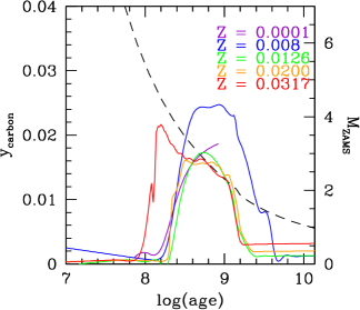
Figure 1: Carbon yields of gas lost from AGB stars for several metallicities calculated by (2004), (2001) and (2005) converted from a function of stellar mass to a function of age by using a star’s lifetime (dashed line). In Gadget-2, we take a star particle’s age and assign the yield from these curves to the fractional amount of mass lost from the star particle and added to the 3 nearest SPH neighbors. The carbon yields jump between $\sim 200$ Myr and 1 Gyr when AGB stars in the range of 2-4 $M_{\odot}$ are dying as carbon stars; AGB yields are highly dependent on age as well as metallicity. The $Z=0.008$ yields show the strongest yields, especially toward lower mass, while by $Z=0.0317$ the strongest yields come from $5M_{\odot}$ stars.

It is worth pointing out that our simulation do not track the metals in stellar remnants. The metal products arising from nucleosynthesis in AGB stars for the most part remain in the white dwarf remnant once it has blown its envelope off, and we do not track the creation of these metals in the star particles. The same is true for neutron stars and stellar black holes. Fortunately these metals remain locked in their stellar remnants on timescales far beyond the age of the Universe, hence we can ignore them as a component of observable metals. When we talk about the global metal budgets in §4, we do not include metals trapped in stellar remnants.

2.2 Group Finder

A group finder added to Gadget-2 allows us to add new dynamics based on the properties of a gas or star particle’s parent galaxy. This is especially important for momentum-driven winds, which MQT05 argued depend on the properties of a galaxy as a whole (specifically a galaxy’s $\sigma$). We will show in §2.3 that winds derived from the group finder more accurately determine wind speeds for the momentum-driven wind model versus using the potential well depth of a particle as a proxy of galaxy mass as was done in OD06 and DO07.

Our group finder is based on the friends-of-friends (FOF) group finder kindly provided to us by V. Springel, which we modified and parallelized to run in situ with Gadget-2. Gas and star particles within a specified search radius are grouped together and cataloged if they are above a certain mass limit, which we set to be 16 gas particle masses. The search radius is set to 0.04 of the mean interparticle spacing corresponding to an overdensity of $(1/0.04)^{3}=15625$. We chose this value after numerous comparisons with the more sophisticated (but far more computationally expensive) Spline Kernel Interpolative DENMAX (SKID) group finder performed on snapshot outputs.

The FOF group finder is run every third domain decomposition, which corresponds to an interval usually between 2 and 10 Myr depending on the dynamical time-stepping for the given simulation (i.e. smaller timesteps for higher resolution). This timestep was chosen to be smaller than the dynamical timescales of most if not all galaxies resolved in a particular simulation. The galaxy properties output include gas and stellar mass and metallicities, star formation rate, and fraction of gas undergoing star formation. The additional CPU cost ranges from 7-10% for a 64-processor run to less than 5% for a 16-processor run. Once the FOF group finder is run, each particle in a galaxy is assigned an ID so that it can be easily linked to all the properties of its parent galaxy.

A comparison plot of the two group finders in Figure 2 for the l32n256vzw-$\sigma$ simulation at $z=0$ shows very good but not perfect agreement for total baryonic galaxy mass ($M_{\rm gal}$, Panel (a)). Galaxies are matched up by requiring a $<5h^{-1}{\rm kpc}$ difference between SKID and FOF positions. Stellar masses ($M_{*}$, lower left panel) are nearly identical, but the associated gas mass ($M_{\rm gas}$, upper right) shows more scatter. Note that there is no explicit density or temperature threshold for including gas in the FOF case, but in the SKID case only gas with overdensities $>1000$ compared to the cosmic mean are included; this may contribute to some of the scatter. FOF group finders have the tendency to group too many things together in dense environments, and this is most noticeable in the associated gas masses. There are significantly better agreements in gas masses at higher redshift, where dense group/cluster environments are less common and gas fractions are greater.

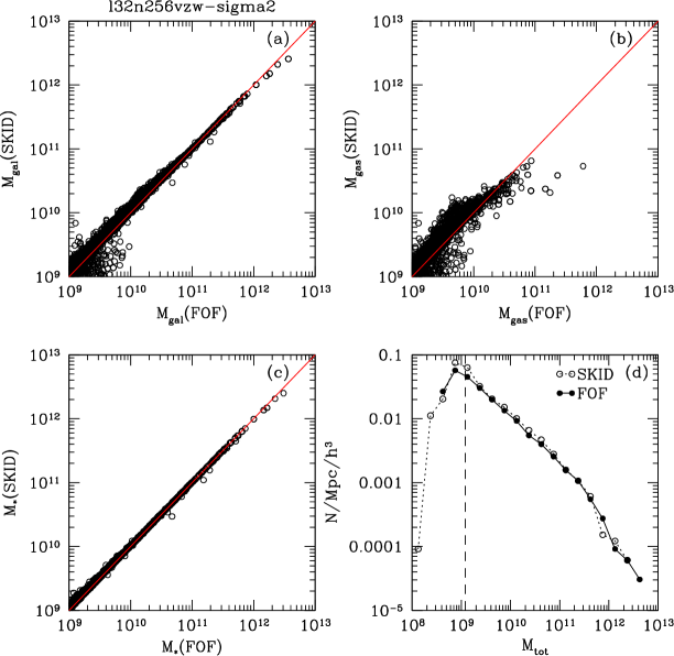
Figure 2: The comparison of two group finders run on a 32 $h^{-1}{\rm Mpc}$ $2\times 256^{3}$ simulation at $z=0$. FOF is the much faster algorithm run in situ with Gadget-2 at frequent intervals to determine galaxy properties on the fly, while SKID is a post-processing DENMAX algorithm run on simulation snapshots. Panels (a), (b), and (c) compare the masses (total, gas, and stellar mass respectively) of groups found within 5 kpc of each other by the two group finders. Stellar masses agree very well while the gas masses (a smaller component by $z=0$) show more scatter. The total mass functions (Panel (d)) of both group finders lie nearly on top of each other above the resolution limit (dashed line), although FOF tends to group some satellites found by SKID with the largest few galaxies. The $M_{\rm gal}$ functions do not resemble a Schechter function, although when one plots $M_{*}$ there is a more pronounced turnover below $M_{*}=10^{10}M_{\odot}$.

The mass functions of both group finders when all galaxies are included show very good agreement (lower right panel of Figure 2). SKID and FOF each find 6 galaxies with $M_{\rm gal}>10^{12}M_{\odot}$, 112 and 113 galaxies with $10^{12}>M_{\rm gal}>10^{11}M_{\odot}$, 793 and 719 galaxies with $10^{11}>M_{\rm gal}>10^{10}M_{\odot}$, and 4296 and 3596 $10^{10}>M_{\rm gal}>10^{9}M_{\odot}$ respectively. $1.2\times 10^{9}M_{\odot}$ is the galaxy mass resolution limit defined as the mass of 64 SPH particles (, 2006). Owing for the tendency of FOF to over-group satellite galaxies with central galaxies in dense environments, there is a deficiency of small satellite galaxies in the FOF case. The total amount of mass in all resolved galaxies is within 0.2% between the two group finders, however there is 24% more mass grouped to the 6 largest galaxies in the FOF finder.

As a side note, our group finder has the flexibility to enable modeling of merger-driven or mass-threshold processes such as AGN feedback. Although our simulations implicitly include both hot and cold-mode accretion (, 2005), (2006) suggests AGN feedback affects only hot mode accretion, and hence there exists a threshold halo mass above which AGN feedback is effective. Our group finder can identify galaxies where AGN feedback may be necessary to curtail star formation and drive AGN winds. Conversely, if AGN feedback is driven by the onset of a merger (, 2005), our group finder can identify mergers and add merger-driven AGN feedback that curtails star formation. We leave such implementations of AGN feedback for future work, though we note that the heating of gas may transport a non-trivial amount of energy and metals into the IGM.

Frequent outputs of the group finder allow us to track the formation history of galaxies to see how galaxies build their mass (e.g. through accretion or mergers). We can trace the star formation rate during individual mergers to see if our simulations are producing bursts of star formation. Outputting group finder statistics during a run allows us to immediately look at integrated properties such as the galaxy mass function, the mass-metallicity relationship, and the specific star formation rate as a function of mass just to name a few. This is valuable as these relations may exhibit changes on timescales shorter than the simulation snapshot output frequency.

2.3 Wind Model Modifications

We use the same kinetic wind implementation of SH03a, whereby particles enter the wind at a probability $\eta$, the mass loading factor relative to the star formation rate. Wind particles are given a velocity kick, ${v_{\rm wind}}$, in a direction given by ${\bf v}\times{\bf a}$ (ie. perpendicular to the disk in a disk galaxy). These particles are not allowed to interact hydrodynamically until either they reach a SPH density less than 10% of the star formation density threshold or the time it takes to travel 30 kpc at ${v_{\rm wind}}$; the first case overwhelms the instances of the second case in our simulations. We admit that this phenomenological wind implementation insufficiently accounts for the true physics of driving superwinds as well as the multi-phase aspect of winds (, 2002, 2005b); see (2008) for an in-depth discussion of some of the insufficiencies of such winds in simulations. However we want to stress that while we cannot hope to model the complexities of the outflows, the focus of this paper primarily depends on the much longer period of subsequent evolution. We use the momentum-driven wind model with variable ${v_{\rm wind}}$ and $\eta$, due to its successes in previous publications mentioned earlier.

In the momentum-driven wind model analytically derived by MQT05, ${v_{\rm wind}}$ scales linearly with the galaxy velocity dispersion, $\sigma$, and $\eta$ scales inversely linearly with $\sigma$. We again use the following relations:

$${v_{\rm wind}} = 3\sigma\sqrt{f_{L}-1},$$ (3)

$$\eta = {\sigma_{0}\over\sigma},$$ (4)

where $f_{L}$ is the luminosity factor in units of the galactic Eddington luminosity (i.e. the critical luminosity necessary to expel gas from the galaxy), and $\sigma_{0}$ is the normalization of the mass loading factor. The outflow models used in this paper are all of the ’vzw’ variety described in §2.4 of OD06, in which we randomly select luminosity factors between $f_{\rm L}=1.05-2.00$, include a metallicity dependence for $f_{\rm L}$ owing to more UV photons output by lower-metallicity stellar populations

$$f_{L}=f_{\rm{L},\odot}\times 10^{-0.0029*(\log{Z}+9)^{2.5}+0.417694},$$ (5)

and add an extra kick to get out of the potential of the galaxy in order to simulate continuous pumping of gas until it is well into the galactic halo (as argued by MQT05).

One difference is that we use $\sigma_{0}=150\;{\rm km}\,{\rm s}^{-1}$ instead of 300 $\;{\rm km}\,{\rm s}^{-1}$ in the equation for $\eta=\sigma_{0}/\sigma\times$SFR. Since our assumed WMAP-3 cosmology produces less early structure that the WMAP-1 cosmology used in OD06, it requires less suppression of early star formation and hence lower mass loading factors (DO07). We find that $\sigma_{0}=150\;{\rm km}\,{\rm s}^{-1}$ with the WMAP-3 cosmology generally reproduces the successes of $\sigma_{0}=300\;{\rm km}\,{\rm s}^{-1}$ with the WMAP-1 cosmology.

The main modification we make to the outflow implementation is how $\sigma$ is derived. Putting the wind parameters in terms of $\sigma$ is the most natural, because the fundamental quantity MQT05 use to derive momentum-driven winds is $\sqrt{GM\over r}$, which equals $\sqrt{2}\sigma$ for an isothermal sphere. In previous runs without a group finder, we derived $\sigma$ using the virial theorem where $\sigma=\sqrt{-{1\over 2}\Phi}$, with $\Phi$ being the gravitational potential at the initial launch position of the wind particle. We will call this old form of the wind model $\Phi$-derived winds. While this derivation of $\sigma$ should adequately work for an isothermal sphere, the $\Phi$ calculated by Gadget-2 is the entire potential: the galaxy potential on top of any group/cluster potential. As galaxies live in groups and clusters more often low redshift, the wind speeds from $\Phi$-derived winds become overestimated. To counteract this trend, we artificially implemented a limit of $\sigma=266$ $\;{\rm km}\,{\rm s}^{-1}$, which corresponds to a $M_{\rm gal}\sim 2.7\times 10^{12}$ $M_{\odot}$, the mass of a giant elliptical galaxy at $z=0$. In the deep potential of a cluster, all galaxies no matter what size would drive winds at the speed of this upper limit. The overestimate of ${v_{\rm wind}}$ prevented us from trusting our wind model at lower redshifts; therefore we usually stopped our simulations in OD06 at $z=1.5$.

We now introduce $\sigma$-derived winds, where $\sigma$ is calculated from $M_{\rm gal}$ as determined by the group finder. We use the same relation as MQT05 (their equation 6) from (1998) assuming the virial theorem for an isothermal sphere:

$$\sigma=200\left(\frac{M_{\rm gal}}{5\times 10^{12}}\frac{\Omega_{m}}{\Omega_{b}}h\frac{H(z)}{H_{0}}\right)^{1/3}\;{\rm km}\,{\rm s}^{-1}.$$ (6)

Since our group finder links only baryonic mass, we multiply $M_{\rm gal}$ by ${\Omega_{m}}/{\Omega_{b}}$ to convert to a dynamical mass. The wind properties are hence estimated from the galaxy alone. We do not calculate $\sigma$ from the velocity dispersion of star and/or gas particles in the galaxy, since our tests show the resolution is insufficient to derive a meaningful $\sigma$.

The $H(z)/H_{0}$ factor in equation 6 increases $\sigma$ for a given mass as $H(z)$ increases at higher redshift. For example, $H(z=6)=10.2\times H_{0}$ resulting in winds being $2.17\times$ as fast being driven from the same mass galaxy at $z=6$ versus $z=0$. Physically, galaxies that form out of density perturbations at higher $z$ have overcome faster Hubble expansion, and therefore their $\sigma$ is higher. The same mass galaxy formed at higher redshift with a higher $\sigma$ means the higher redshift galaxy must be more compact. Such a scenario is supported by the observations by (2006) and (2007) showing a trend of galaxies becoming smaller from $z=0\rightarrow 2$, in general agreement with (1998). A more compact galaxy drives a faster wind in the momentum-driven wind model, because ${v_{\rm wind}}$ is a function of $M_{\rm gal}/r$, not just $M_{\rm gal}$; there is more UV photon flux impinging each dust particle. We will show that increasing ${v_{\rm wind}}$ emanating from the same mass galaxy toward higher $z$ has important consequences in enriching the IGM at high-$z$ while not overheating it at low-$z$.

Another modification to the wind model we add are new ${v_{\rm wind}}$ speed limits. The first depends on the star formation timescale, $\tau_{\rm SFR}$. The momentum-driven wind equation derived by MQT05 and used in OD06 and DO07 assumes a starburst occurs on the order of a dynamical timescale, $\tau_{D}$, which is often the case in a merger-driven starburst. However, MQT05 also derive a maximum $\sigma$, $\sigma_{\rm max}$, above which a starburst cannot achieve the luminosity needed to expel the gas in an optically thick case. Although it is not clear how $\sigma_{\rm max}$ varies with the $\tau_{\rm SFR}$, we modify their equation 23 to have an inverse linear dependence on the star formation timescale

$$\sigma_{\rm max}=4000\times\frac{\tau_{\rm D}}{\tau_{\rm SFR}}\;{\rm km}\,{\rm s}^{-1}$$ (7)

and assume a $\tau_{D}$ of 50 Myr. The end result is a reduction of 5-10% in the average ${v_{\rm wind}}$ out of $M_{\rm gal}\sim 10^{12}$ at $z<1$.

A second speed limit we impose allows no more than $2\times$ the total SN energy to be deposited into the wind. This does not violate the energetics as the energy for these winds is coming from momentum deposition over the entire lifetime of a star, which is of the order $100\times$ the SN energy (, 2003). This limit was instituted to disallow extreme values of ${v_{\rm wind}}$ (i.e. $>1500\;{\rm km}\,{\rm s}^{-1}$) emanating from the most massive haloes, reducing ${v_{\rm wind}}$ at most 30-50% in the most massive galaxies at $z<1$.

In Figure 3, we plot the average wind speed, $\langle{v_{\rm wind}}\rangle$, as a function of galaxy mass at four redshifts for a variety of box sizes ranging from 8 to 64 $h^{-1}{\rm Mpc}$ along. Dotted lines show the predicted $\langle{v_{\rm wind}}\rangle$ for solar metallicity, assuming no speed limits. As with every plot in this paper, $M_{\rm gal}$ is the SKID-derived baryonic mass, not the FOF-derived mass from which ${v_{\rm wind}}$ is calculated. The simulations reproduce the predicted trend ${v_{\rm wind}}\propto M_{\rm gal}^{1/3}$. Divergences at low mass result from faster winds being driven by low-mass, low-metallicity galaxies as well as some satellites being grouped with a central galaxy in groups/clusters by FOF. The latter effect appears to be sub-dominant though as evidenced by the overlap of the relation among simulations at different redshifts. The deviations at the high-mass end at all redshifts are dominated by the second wind speed limit discussed above.

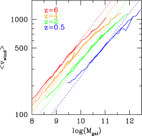
Figure 3: Average launch wind speed as a function of $M_{\rm gal}$ (derived using SKID) versus dotted lines for the predicted $\langle{v_{\rm wind}}\rangle$ assuming no speed limits. The wind speeds, which are derived using the FOF finder during a run, agree very well with the masses determined by SKID in the post-processing stage. The decline in $\langle{v_{\rm wind}}\rangle$ with redshift for a given $M_{\rm gal}$ is a result of the $H(z)$ dependence in equation 6. This trend loosely matches observations of faster winds for a given mass galaxy at high redshift.

The reduction in ${v_{\rm wind}}$ for a given mass galaxy due to the $H(z)$ dependence in equation 6 is the reverse of the trend in the $\Phi$-derived models, and are in better agreement with low-$z$ observations. In the new $\sigma$-derived wind model, a $10^{11}M_{\odot}$ galaxy (such as the Milky Way) launches an average wind particle at 790 $\;{\rm km}\,{\rm s}^{-1}$ wind at $z=3$ and 450 $\;{\rm km}\,{\rm s}^{-1}$ at $z=0$ while the corresponding values for the $\Phi$-derived winds without any speed limits are 1040 $\;{\rm km}\,{\rm s}^{-1}$ and 1220 $\;{\rm km}\,{\rm s}^{-1}$ respectively. The latter are far above the values observed in the local Universe. (2005a) found the relation $v_{\rm term}\propto 2.1\times v_{\rm circ}$ fit her observations best, where $v_{\rm term}$ is the terminal velocity of the wind. For a $10^{11}M_{\odot}$ galaxy, this corresponds to $v_{\rm circ}\sim 125$ $\;{\rm km}\,{\rm s}^{-1}$ leading to $v_{\rm term}\sim 265$ $\;{\rm km}\,{\rm s}^{-1}$. This is much nearer our $\sigma$-derived value once the extra velocity boost to leave the potential of the galaxy is subtracted. High-velocity clouds (HVC’s) may be material that is blown into the halo from the Milky Way (, 1997), and these have velocities that are $\ll 1000\;\;{\rm km}\,{\rm s}^{-1}$, in better agreement with velocities expected in the $\sigma$-derived model. Of course the Milky Way is not a star-bursting galaxy driving a powerful wind; however, it is still possible that it is kicking up a significant amount of gas into the halo. Indeed, as we will discuss later (§5.4), the outflows in our simulations don’t always reach the IGM, but particularly at low-$z$ may be more aptly described as “halo fountains”, where the outflows only propagate out to distances comparable to the galactic halo.

It remains very difficult to determine from observations whether wind speeds increase for a given mass galaxy at high-$z$ as the $\sigma$-derived winds predict. Observing asymmetric Lyman-$\alpha$ profiles,(2005) find what they interpret as 290 $\;{\rm km}\,{\rm s}^{-1}$ outflows around a LBG with $10^{11}M_{\odot}$ baryons at $z=3.09$. More recently (2007) observe outflows up to 500 $\;{\rm km}\,{\rm s}^{-1}$ at $z=4.88$ around a lensed galaxy with a dynamical mass as low as $10^{10}M_{\odot}$. These observed outflows appear to be beyond the virial radius in both cases and correspond to our velocities once we have subtracted the extra velocity boost we add to get out of the potential well. Our $v_{\rm term}$ for the (2005) $z=3$ galaxy would be closer to $500\;{\rm km}\,{\rm s}^{-1}$, somewhat above their observed values. We expect ${v_{\rm wind}}\sim 300\;{\rm km}\,{\rm s}^{-1}$ ($v_{\rm term}\sim 200$ $\;{\rm km}\,{\rm s}^{-1}$) for the (2007) object, but their mass is only a lower limit. If this object is a $10^{10}M_{\odot}$ baryonic-mass galaxy, we would derive $v_{\rm term}\sim 400\;{\rm km}\,{\rm s}^{-1}$. Overall, the $\sigma$-derived winds predict velocities that are at least in the ballpark of observed values. Additionally, surveys of LBG’s at$z\sim 3$ (, 2001, 2003) find outflows of several hundred $\;{\rm km}\,{\rm s}^{-1}$ to be ubiquitous, often driving an amount of mass comparable to the star forming mas (i.e. $\eta\sim 1$)

3 The Universal Energy Balance

Armed with these new simulations, we can now investigate how outflows move mass, metals, and energy around the Universe. In this section we focus on the energetics of outflows, and its impact on cosmic star formation and temperature. We will compare the new $\sigma$-derived wind model’s behavior versus the old $\Phi$-derived wind model, and study the impact of AGB feedback. Specifically, $\sigma$-derived winds inject much less energy at late times making a cooler and less-enriched IGM while leading to more star formation. The inclusion of AGB feedback does not really affect the global energy balance, but does increase the number of stars formed and more significantly affects the amount and location of metals, as we discuss in §4.

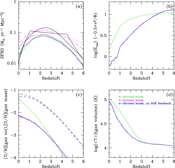
Figure 4: Three 32 $h^{-1}{\rm Mpc}$ $2\times 128^{3}$ simulations: $\Phi$-derived winds including AGB feedback (green), $\sigma$-derived winds with AGB feedback (magenta), and $\sigma$-derived winds without AGB feedback (blue) demonstrate how global quantities evolve as a result of energetic interactions between star formation-driven feedback from galaxies and the state of the IGM. Panel (a) shows the star formation density histories compared to the (2006) compilation averages (black lines for segmented and non-segmented fit, scaled to a Chabrier IMF). Panel (b) shows the average virial ratio with which wind particles are launched. Solid/dashed lines in Panel (c) trace the volume/mass-weighted average gas oxygen content, and Panel (d) shows the volume-weighted temperature. The new $\sigma$-derived winds do not inject as much energy or metals into the IGM while increasing the star formation. AGB feedback has a relatively minor effect in the energetic balance between galaxies and the IGM. The lower resolution l32n128 simulation misses about half of all star formation, therefore we also show the l32n256 (dash-dotted line) and the l16n256 (dotted line) simulations in Panel (a), which both agree better with observations.

The history of the cosmic star formation rate density (SFRD; , 1996, 1996) is a key observable that has received much attention in recent years (e.g. , 2006, 2007). The SFRD plot in the upper left panel of Figure 4 shows how our models compare to the (2006) compilation (black lines, two different fits). It should be noted that we are resolving galaxies down to $\approx 10^{10}M_{\odot}$ in the models shown with solid lines, and hence the star formation density at $z\ga 3$ is increasingly underestimated (see e.g. SH03b). Hence this should be considered as an illustrative comparison, whose main point is to highlight the differences between various models. A more complete SF history at early times is shown by the dashed and dotted magenta lines from our higher resolution $2\times 256^{3}$ particle simulations with $\sigma$-derived winds with AGB feedback. The metal enrichment of the IGM at early times is significantly higher when the star formation from smaller galaxies is included; therefore we use only higher resolution models to explore the IGM enrichment at $z>2$. Also, our models suggest an overestimated SFRD at the lowest redshifts. This indicates that some other form of feedback is needed to suppress star formation in massive galaxies at late times (such as AGN feedback; e.g. , 2007).

The three models shown, the $\Phi$-derived winds and the $\sigma$-derived winds with and without AGB feedback, are indistinguishable in their global SFRD’s above $z=4$ because the mass loading factor and not wind speed is the largest determinant of star formation (OD06). As explained in OD06, the earliest wind particles have not had time to be re-accreted by galaxies, therefore the SFR is regulated purely by how much mass is ejected ($\eta$). The faster wind velocities of the $\Phi$-derived model at $z<2$ decrease star formation relative to the $\sigma$-derived model, because wind particles are sent further away from galaxies making this gas harder to re-accrete while also heating the IGM more and further curtailing star formation. We will quantify this recycling of winds in §5.

The average virial ratio of winds ($E_{\rm rat}$), defined as the ratio of the kinetic energy to the potential at the launch position ($0.5\times{v_{\rm wind}}^{2}/-\Phi$), in the upper right panel shows how $\sigma$-derived winds inject progressively less energy into their surroundings with time. $E_{\rm rat}$ should be invariant across time for $\Phi$-derived winds in its simplest form, but falls sharply below $z=1$ due to our wind speed limits, and rises slightly at high-$z$ due to the metal dependent ${v_{\rm wind}}$. The faster $\Phi$-derived winds spatially distribute more metals (solid lines in lower left panel) and heat the IGM (lower right panel) to a greater extent than the $\sigma$-derived winds. We will show in §4.2 that the cooler, less-enriched IGM of the $\sigma$-derived wind models makes a significant difference in metals seen in quasar absorption line spectra. The gaseous metallicity (dashed lines in lower left panel) is slightly higher in the $\Phi$-derived wind model despite fewer overall stars formed, because fewer metals end up in stars.

Finally, we consider the impact of AGB feedback. AGB stars do not add any appreciable energy feedback, as demonstrated by the invariance in the $E_{\rm rat}$ and volume-averaged temperature in the models with (magenta lines) and without (blue) AGB feedback. However, AGB stars provide feedback in the form of returning gas mass to the ISM, which is now available to create further generations of stars. For instance, with AGB feedback the SFRD at $z=0$ is increased by nearly a factor of two compared to without. Hence models that do not include such stellar evolutionary processes may not be correctly predicting the SFRD history.

4 The Universal Metal Budget

In this section, we will investigate what the sources of cosmic metals are, and where these metals end up. To do so, we examine quantities summed over our entire simulation volumes, with special attention to the three different sources of metals: Type II SNe, Type Ia SNe, and AGB stars. We also discuss the impact of AGB feedback and $\sigma$-derived winds.

4.1 Sources of Metals

4.1.1 The Stellar Baryonic Content

Since stars produce metals, we first examine the evolution of the stellar baryonic content. The key aspect for metal evolution is that stellar recycling provides new fuel for star formation. For the Chabrier IMF assumed in our simulations, supernovae return $\sim 20\%$ of stellar mass instantaneously back into the ISM (which is double that for a Salpeter IMF), and delayed feedback will eventually return another $\sim 30\%$ over a Hubble timescale. With half the gas being returned to the ISM, most of it ($\sim 80\%$) on timescales of less than a Gyr, subsequent generations of stars can form, leading to greater metal enrichment. The difference between $\sigma$-derived wind models with and without AGB feedback in the SFRD plot (upper left panel of Figure 4) demonstrates how AGB feedback makes available more gas for star formation at later times.

Despite more star formation in the l64n256vzw-$\sigma$ model with AGB feedback, slightly more mass is in stars at $z=0$ in the no-AGB feedback model by $z=0$ ($\Omega_{*}(z=0)/\Omega_{b}=0.081$ vs. 0.071) since there is no mass loss from long-lived stars. However, if we count all stars (including short-lived stars undergoing SNe) formed over the lifetimes of our simulated universes, the AGB feedback model forms 37% more stars ($\Omega_{*}(all)/\Omega_{b}=0.138$ vs. 0.101). This is the more relevant quantity when considering the metal budget of the local Universe. Another way to think of this is that the stars in today’s local Universe account for ($\Omega_{*}(z=0)/\Omega_{*}(all)$=) 52% of all the stars that have ever existed, assuming the mass in short-lived stars is negligible (a safe assumption in the low-activity local Universe).

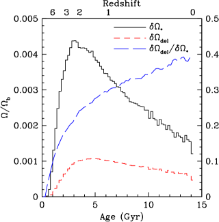
Figure 5: Global quantities binned in 200 Myr bin of stars formed ($\delta\Omega_{*}$, solid black line) and mass lost via delayed feedback ($\delta\Omega_{\rm del}$, dashed red line) relative to $\Omega_{b}$ in the 32 $h^{-1}{\rm Mpc}$ $2\times 256^{3}$ simulation. The ratio of the two is the long-dashed blue line.

Figure 5 shows the amount of baryons formed into stars, $\delta\Omega_{*}$ (i.e. the star formation rate), and the amount of stellar mass lost via delayed feedback, $\delta\Omega_{\rm del}$, as a function of time. The ratio $\delta\Omega_{\rm del}/\delta\Omega_{*}$ increases as more generations of stars are continuously formed with each generation contributing to $\delta\Omega_{\rm del}$. The quantity $\delta\Omega_{\rm del}/\delta\Omega_{*}$ should approach 0.3 for a steady star formation rate in a Hubble time, because 30% of the stellar mass is returned via delayed feedback, but this is actually exceeded since the star formation is declining at late times. The amount of material lost via delayed feedback over the history of the Universe is found by subtracting the stars at $z=0$ from the number of long-lived stars formed over the history of the Universe.

$$\Omega_{\rm del}=\int_{0{\rm Gyr}}^{14{\rm Gyr}}\delta\Omega_{*}(t)(1-f_{\rm SN})dt-\Omega_{*}(z=0)$$ (8)

where we assume $\Omega_{*}(z=0)$, the stars in today’s Universe, has a negligible quantity of short-lived stars. The amount of delayed feedback is $\Omega_{\rm del}=0.039$ or 55% of the stellar baryons in today’s Universe, which is a significant quantity.

4.1.2 The Metal Content

We segue into our discussion of metals by plotting the global production of the 4 species tracked by their source (Type II SNe, Type Ia SNe, or AGB stars) in the left panels of Figure 6. Metals produced by Type II SNe depend on the current star formation rate ($\delta\Omega_{*}$), which is apparent by the fact that the solid lines in the left panels have roughly the similar shape to the global stellar mass accumulation rate (Figure 5). Type II SNe dominate the enrichment for all four elements at all redshifts, hence global chemical enrichment is reasonably approximated by current star formation alone.

Dividing the amount of each type of metal formed via Type II SNe by $\Omega_{*}$ gives the SN yield of that element shown as solid lines in the right panels of Figure 6. These yields should and do match the Type II SNe yield tables that are an input to the simulations. The yields do not evolve significantly because there is only weak metallicity dependence in the (2005) yields employed here. Note that previous work has generally assumed no metallicity dependence. Above $z=6$, the yields are slightly lower due to less metals injected by low-metallicity stars. A slight upturn is noticeable at lower redshift for carbon and silicon as their yields increase with metallicity.

Turning to metals injected via AGB feedback (dashed red lines in Figure 6), we find more complex behavior that varies among the species. The left panels show that AGB feedback is an important source of carbon ($\sim 30\%$ by $z=0$), iron and silicon (both $\sim 25\%$ by $z=0$), but is a negligible contributor for oxygen. Dividing these values by $\Omega_{\rm del}$ results in the global AGB yields as a function of redshift in the right panels. For carbon and oxygen, these are a summation of the yield values in our input tables for all stars of various ages and metallicities undergoing AGB feedback.

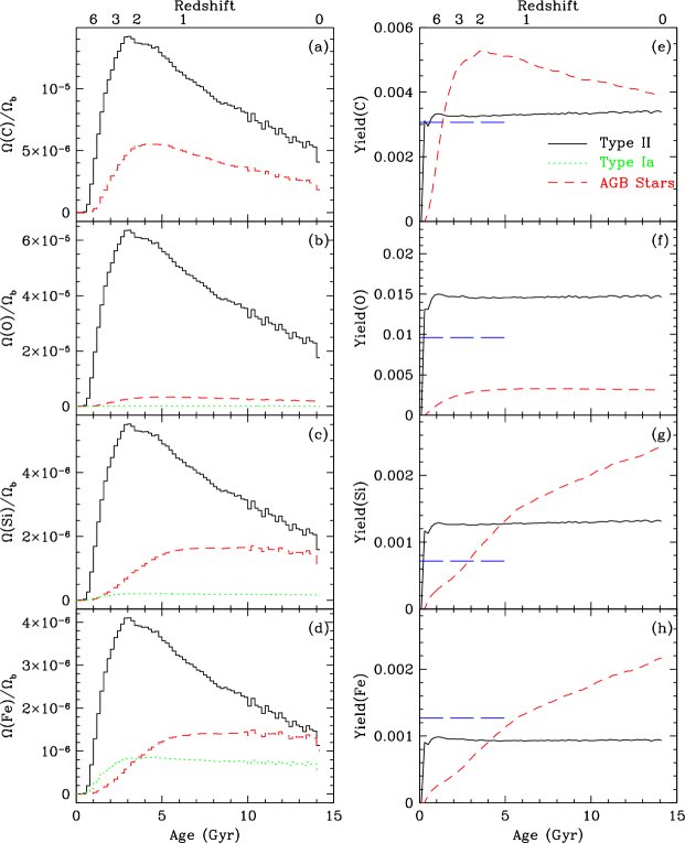
Figure 6: Metal production by species relative to $\Omega_{b}$ along with their yields plotted in 200 Myr bins in the 32 $h^{-1}{\rm Mpc}$ $2\times 256^{3}$ simulation. Panels (a-d) trace the amount of carbon, oxygen, silicon, and iron respectively returned to the gas phase by Type II SNe (black solid lines), Type Ia SNe (green dotted lines), and AGB stars (red dashed lines). The yields for the various species are calculated in Panels (e-h) by taking lines in Panels (a-d) and dividing by the matching line types in Figure 5; long dashed lines on the left indicate (1989) solar values. Type II SNe yields remain relatively constant despite metallicity-dependent yields. The AGB carbon yields strongly depend on $z$ and peak when 2-4 $M_{\odot}$ die. AGB silicon and iron yields are simply reprocessed metals formed in SNe and reflect the ensemble metallicities of all stars undergoing AGB feedback at a given redshift.

The carbon yields shows the most interesting evolution, which are indicative of the underlying processes of stellar evolution in different stars. As explained in §2.1.3 and shown in Figure 1, the most massive and short-lived AGB stars (4-8 $M_{\odot}$) have hot-bottom burning that destroys carbon; these are the stars losing mass via AGB feedback the most at very high-$z$. Between 2-4 $M_{\odot}$, the third dredge-up makes AGB stars into carbon stars with very high carbon yields from stars dying 200 Myr to 1 Gyr after their formation. At $z\sim 2$, carbon stars dominate the carbon yields, but then less massive stars ($<2M_{\odot}$) without the third dredge-up begin to reach the AGB phase, and the ensemble AGB carbon yield begins to decline.

Oxygen is burned in AGB stars, resulting in a net decrease in its overall content as a result of delayed feedback. Accounting for a minor contribution from Type Ia SNe, the vast majority of gaseous oxygen is synthesized in Type II SNe. Hence oxygen is the ideal species to trace the cosmic evolution of Type II SNe.

The AGB yields of silicon and iron may at first be surprising considering that AGB stars do not process these elements. These yields reflect the ensemble metallicities of mass loss from AGB stars, since they neither create nor destroy heavier elements at any significant rate, but instead simply regurgitate them. Most surprising is that more iron is ejected from AGB stars than Type Ia SNe. The difference between these two forms of feedback associated with stars is that the iron yield of Type Ia SNe is nearly a half (i.e. 0.6 $M_{\odot}$ formed per 1.4 $M_{\odot}$ SNe) and should significantly enrich its local environment, while the iron lost from AGB stars should have a slightly lower yield than the surrounding gas metallicity since these stars are older and hence less enriched.

It is curious and probably not correct that iron and silicon AGB yields exceed solar metallicities by as much a factor of $2-3$ by $z=0$. This means that at $z=0$, the average AGB star is at least $2-3\times Z_{\odot}$, which is almost definitely too high when stars younger than the Sun in the Milky Way disk are $\sim Z_{\odot}$ (, 1980). Even though most $z=0$ AGB mass loss comes from stars younger than the Sun since most AGB feedback occurs within 1 Gyr for a Chabrier IMF, the extremely super-solar metallicities are indicative of too much late star formation. Reasons for this include too much star formation in massive systems in our simulations, as well as our slightly high value of $\Omega_{b}=0.048$ (instead of the currently more canonical $\Omega_{b}=0.044$).

Table 2 summarizes the sources of metals at $z=2$ (roughly $10^{10}$ years ago) and $z=0$ for the l32n256vzw-$\sigma$ simulation. These can be compared to available observational constraints. Using oxygen, the global metallicity averaged over all baryons is $\langle Z_{b}\rangle(z=2)\sim 0.064Z_{\odot}$ rising to $\langle Z_{b}\rangle(z=0)\sim 0.23Z_{\odot}$. These values are remarkably similar to those derived by (2007) (hereafter B07) ($\langle Z_{b}\rangle(z=2)\sim 0.056$ and $\langle Z_{b}\rangle(z=0)\sim 0.20Z_{\odot}$) where they assumed a Salpeter IMF-weighted metallicity yield of 0.024 and integrated over the star formation history of the Universe from (2001). While encouraging, this comparison is highly preliminary owing to many systematics, such as the fact that our simulations produce too many stars overall, and the assumption of a Salpeter IMF at all times is probably not consistent with observations (see e.g. , 2008, and discussions therein). It is hoped that improving observations will enable more interesting constraints on cosmic chemical evolution models.

Table 2: Sources of Feedback

Species	$\Omega/\Omega_{b}$	% Type II	% Type Ia	% AGB Stars	% AGB Processing
$z=2$
Baryons	–	0.87	.0016	0.83	–
Carbon	1.677e-04	85.70	0.0a	23.25	+14.30
Oxygen	6.123e-04	105.4	0.32	3.48	-5.75
Silicon	5.642e-05	96.50	3.57	9.30	+0.00
Iron	5.013e-05	83.49	16.51	9.23	+0.00
$z=0$
Baryons	–	3.74	.0098	5.42	–
Carbon	6.566e-04	95.35	0.0a	38.29	+4.65
Oxygen	2.194e-03	126.1	0.52	7.68	-26.60
Silicon	2.549e-04	95.29	4.72	33.89	+0.00
Iron	2.265e-04	78.32	21.68	33.16	+0.00

^aThese models were run with no Type Ia yields for carbon. These carbon yields are fractionally insignificant anyway.

While it is well-known that Type II SNe dominate carbon, oxygen, and silicon production, it may be somewhat surprising for iron, considering that Type Ia SNe are often assumed to be the primary producers of iron; however, this is actually only true in environments dominated by older stars. Long-lived stars also destroy oxygen, eliminating 20% of the oxygen formed by Type II SNe. Processing of oxygen by AGB stars helps to move oxygen abundances from alpha-enhanced levels to solar levels. Of course, long-lived stars do make a net surplus of both carbon and oxygen in post-Main Sequence nucleosynthesis, however most of these metals remain locked in stellar remnants, which we do not track in our simulations and are not included in this table. (2004) estimate a $\langle Z_{b}\rangle(z=0)\sim 0.68Z_{\odot}$ for all metals including those in remnants, which exceeds the metals not locked up (i.e. the ones we track) by a factor of a few.

Even though AGB feedback injects an appreciable amount of carbon into surrounding gas ($\sim 40$% of carbon injected via Type II SNe), the net surplus of carbon resulting from AGB feedback is only $\sim 5$% of Type II SNe by $z=0$, because much of this carbon is coming from stars with high metallicity already. Carbon stars ($\sim 2-4M_{\odot}$) add to the overall cosmic carbon abundance while higher and lower mass AGB stars reduce the amount of carbon. A larger impact on carbon production comes from recycled gas that enables more Type II SNe; as noted before, 37% more stars form in simulations that include AGB feedback. Stars also lose mass via AGB feedback when they have moved away from the sites of their formation, and can directly enrich metal-poorer areas such as the ICM and intra-group medium. Hence the location of feedback from AGB stars and Type Ia SNe turns out to be important for understanding enrichment in various environments. We consider this topic next.

4.2 The Location of Metals

B07 calculated from observations that metals migrated from gas to stars between $z=2\rightarrow 0$ as metals fall back into the deeper potential wells of growing galaxies, and are more likely to remain there as star formation-driven winds decline at low-$z$. Our new simulations generally agree with the results of B07 that about one-third of metals are in stars at $z=2$, increasing to two-thirds by $z=0$.

In Figure 7 we subdivide mass and metals further by their baryonic phases. The top panel shows the baryonic fraction in diffuse gas ($T<10^{5}$), warm-hot intergalactic medium (WHIM) gas ($10^{5}<T<10^{7}$), hot gas in clusters ($T>10^{7}$), and galaxies (stars and ISM) for both the l64n256vzw-$\sigma$, l64n256vzw-$\sigma$-nagb, l32n128vzw-$\Phi$ models as a function of redshift. The steady transfer of gas from diffuse to WHIM and hot IGM between $z=3\rightarrow 0$ was first noted by (1999) and (1999), and our current results are similar to those from (2006) using nearly the same cosmology. The addition of AGB feedback does not appreciably change any of these values.

$\sigma$-derived winds have 5% fewer baryons in the WHIM than $\Phi$-derived winds at $z=0$ due to weaker winds at late times. (2006) find that their baryon fraction in the WHIM increases by about 10% owing to galactic superwinds, which matches our results (not shown). The metal fraction in the WHIM is basically constant in the $\sigma$-derived winds, in stark contrast to the $\Phi$-derived wind model (green lines; also see Figure 1 of DO07), which shows that fraction of metals in WHIM grow steadily from $z=4\rightarrow 0$, reaching 25% today. The much slower $\sigma$-derived wind velocities at late epochs are mostly unable to shock-heat metals above temperatures where metal-line cooling dominates, and instead the gas cools efficiently. Although the addition of AGN feedback is unlikely to change the metal content of baryons by more than a few percent (B07), the effect of $>1000$ $\;{\rm km}\,{\rm s}^{-1}$ winds from QSO’s such as those observed by (2007) could be appreciable for metals in the WHIM and hot phases.

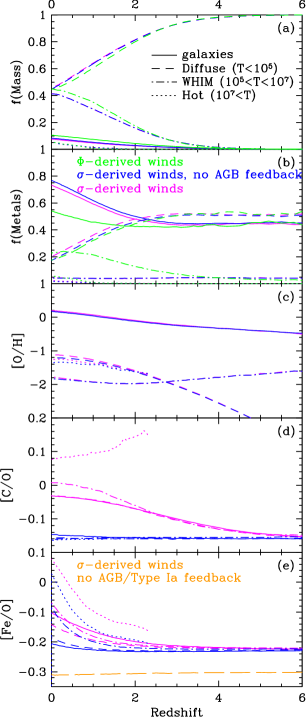
Figure 7: The evolution of of mass and metals by baryonic phase in the 64$h^{-1}{\rm Mpc}$, $2\times 256^{3}$ simulations with and without AGB feedback, and the 32$h^{-1}{\rm Mpc}$, $2\times 128^{3}$ simulation with the old potential-derived winds (shown only in top two panels). The slower $\sigma$-derived winds at low redshift do not inject nearly as many metals into the WHIM. The addition of AGB feedback does not change the baryonic mass fractions (Panel a) and increases slightly the amount of metals in galaxies (Panel b). Oxygen metallicity (Panel c), which traces Type II SNe, remains nearly unchanged, but delayed feedback boosts carbon relative to oxygen (Panel d), and iron is increases at late times relative to oxygen (Panel e) in hot gas mostly due to Type Ia SNe. The global [Fe/O] in a test simulation without any delayed feedback is shown as the long dashed orange line in Panel (e).

The total metal budget by baryonic phase in the second panel shows a minor change owing to AGB feedback, namely that 5% less metals are found in the galaxies, with those metals instead being located in the diffuse IGM. This is because increased star formation from gas made available via delayed feedback results in more winds that expel metals.

4.2.1 Oxygen in the WHIM

The third panel of Figure 7 shows the oxygen metallicity in various baryonic phases. Overall, oxygen metallicities ([O/H]) remain nearly identical (within 0.1 dex) with the addition of AGB feedback. The 37% increase in star formation and therefore oxygen production from Type II SNe is counterbalanced by a 20% decrease due to the AGB processing of oxygen. Galactic baryons show slightly super-solar oxygen abundance, while the abundances in diffuse and hot phases are nearly one-tenth solar.

The WHIM oxygen abundance is relatively constant with redshift, and shows [O/H]=$-1.76$ at $z=0$. Our simulations produce two distinct types of WHIM: (1) the unenriched majority formed via the shock heating resulting from structural growth, and (2) the WHIM formed by feedback, which is significantly enriched. The weaker $\sigma$-derived winds form very little of the latter. While simulations suggest, by comparison with observed O vi absorbers, that the WHIM metallicity should be around one-tenth solar (, 2001, 2003), it remains to be seen whether the $\sigma$-derived winds are in conflict with O vi observations. Since O vi arises in both photoionized and collisionally-ionized gas, it could be that enough O vi is present in photoionized gas to explain the observed number density of such systems. Moreover, non-equilibrium ionization effects could be important (, 2006). A careful comparison with O vi observations is planned, but is beyond the scope of this paper.

For now, we note that the oxygen abundance in the WHIM may be an interesting probe of feedback strength. (2008) come to the same conclusion at $z=3$ when tracing oxygen content by temperature, noting that the stronger feedback by a top-heavy IMF produces significantly greater amounts of oxygen in the WHIM. Extremely fast winds (${v_{\rm wind}}>1000\;{\rm km}\,{\rm s}^{-1}$) emanating from AGN (, 2007) will also create more enriched WHIM.

4.2.2 Carbon in the IGM

In the bottom two panels of Figure 7 we show the carbon and iron abundance relative to oxygen, a tracer of Type II SNe enrichment, to emphasize the differences in these two species influenced by delayed feedback. For carbon especially, AGB feedback has a significant impact. [C/O] evolution shows an obvious increase even at high-$z$, because the timescale for mass loss from carbon stars is $0.2-1$ Gyr. Every phase appears to evolve similarly with their lines sometimes blending in Figure 7 except the hot phase, which has at least 50% more carbon at $z>2$ . Carbon stars lose their mass near sites of star formation, and this carbon is then blown out and shock-heated by a second generation of supernovae. The net effect of AGB feedback on the $z=0$ carbon metallicity is +0.22, +0.25, and +0.33 dex for diffuse, WHIM, and hot IGM respectively. This results in abundance ratios close to solar in all phases.

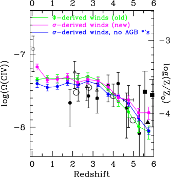
Figure 8: Evolution of $\Omega$(C iv) from $z=6\rightarrow 0$ for the $\Phi$-derived wind model with AGB feedback (green) and the $\sigma$-derived wind model with and without AGB feedback (magenta and blue). Our models are compared to observations from (2001) (black circles), (2003) (small filled black squares), (2003) (open triangles), (2003) (open square), (2005) (large open dots), (2006) (large black squares), and (2006) (black triangle is a lower limit). While all models appear to fit the majority of the data, there are subtle differences that we highlight between our models. The new $\sigma$-derived winds distribute metals more broadly boosting $\Omega$(C iv) at $z>5$, while more carbon resulting from AGB feedback enriches the IGM in the local Universe. The three data points below $z=1.5$ are calculated from 8 $h^{-1}{\rm Mpc}$ $2\times 128^{3}$ simulations and from 16 $h^{-1}{\rm Mpc}$ $2\times 256^{3}$ elsewhere, except in the case of the $\sigma$-derived winds without AGB feedback in which case only the small box is used.

A basic observational test of IGM enrichment models is the evolution of $\Omega$(C iv), i.e. the mass density in C iv systems seen in quasar absorption lines. In Figure 8 we plot $\Omega$(C iv) from $z=6\rightarrow 0$ (see OD06 for exact method of computing $\Omega$(C iv)) to see the effect of $\sigma$-derived winds and AGB feedback. In OD06 we reproduced the relative invariance in the observed trend of $\Omega$(C iv) between $z=5\rightarrow 2$ by counterbalancing the increasing IGM carbon content by a similarly lowering C iv ionization factor; the new $\sigma$-derived models also match the observed trend quite well, for a similar reason. The addition of AGB feedback increases $\Omega$(C iv) by 70% (+0.23 dex) at $z\la 0.5$, leading to a value consistent within the error bars of $z\approx 0$ measurement by (2003).

The main reason is that AGB feedback adds new fuel for star formation, resulting in more C iv expelled into the IGM at late times. Compared to the $\Phi$-derived winds, the $\sigma$-derived winds push out more metals early better matching the high-$z$ C iv observations of (2006) and (2006). The faster $\Phi$-derived winds at low-$z$ raise the temperature of the metal-enriched IGM while pushing the metals to lower overdensities and lowering the C iv ionization fraction.

The $\sigma$-derived wind model with AGB feedback is the first model we have explored that is able to fit the entire range of $\Omega$(C iv) observations from $z\sim 6\rightarrow 0$.

The $\sigma$-derived wind model with AGB feedback achieves higher $\Omega$(C iv) at $z>5$ and $z<1$ that at face value improves agreement with observations. While these data are uncertain and hence one should not over-interpret this improved agreement, the main point of this exercise is to show how our newly incorporated physical processes could have observational consequences. Furthermore, the results are to be taken with caution, owing to the small box size of our simulations (8 $h^{-1}{\rm Mpc}$ $2\times 128^{3}$) below $z=1.5$; this volume is not nearly large enough to form the large-scale structures in the local Universe. It is encouraging that the values derived from this small box agree within the error bars with the larger l16n256vzw-$\sigma$ simulations above $z=1.5$. Future observations at low-$z$ by the Cosmic Origins Spectrograph, and at high-$z$ with advances in near-IR spectroscopy will allow more relevant and detailed comparisons.

4.2.3 Iron in the ICM

The [Fe/O] evolution (bottom panel of Figure 7) is dominated by Type II SNe until $z\sim 2$, at which point delayed feedback processes of Type Ia SNe and AGB stars become important. The instantaneous component of the Type Ia SNe adds 19% of the Type II SNe iron yield, which raises the [Fe/O] everywhere from -0.30 to -0.23 (compare to global [Fe/O] in a simulation without any Type Ia’s or AGB feedback). The delayed component of Type Ia SNe adds only 9% more of the Type II SNe iron content generated over the lifetime of the Universe. However, the combination of the high iron yield (0.43) and the location of enrichment often being low-metallicity regions away from the sites of star formation meas delayed Type Ia’s can have a significant observational signature in a low-density medium such as the ICM. The net increase of all Type Ia SNe (delayed and instantaneous) on the $z=0$ iron content is +0.32 dex in the hot component and +0.21 dex in the WHIM. AGB feedback increases iron content by allowing 37% more stars to form; this extra iron primarily remains in galaxies, but increases iron in the hot component by +0.15 dex and the WHIM by +0.07 dex. Overall, the hot iron metallicity increases by nearly 3$\times$ with the addition of Type Ia and AGB feedback.

To demonstrate the effect on observables, we calculate the free-free emission-weighted [Fe/H] of the ICM in clusters/groups with temperatures in excess of 0.316 keV at $z=0$ in the l64n256vzw models to simulate the X-ray observations. We identify large bound systems in the simulations using a spherical overdensity algorithm (see , 2006, for description). The average of over 130 clusters/groups is -1.11 without any delayed feedback, -0.78 with Type Ia SNe included, and -0.57 with AGB feedback also included. Hence the addition of delayed forms of feedback increases the ICM [Fe/H] by $3.4\times$. This is now in the range for the canonical ICM metallicities of around 0.3 solar, as well as for groups between 0.316 and 3.16 keV as observed by (2000) (they found $-0.60<$[Fe/H]$<-0.36$). Of course, X-ray emission at $\sim 1$ keV has a significant contribution from metal lines, and observations can be subject to surface brightness effects (e.g. , 2000), so this comparison is only preliminary. A more thorough comparison of simulations to ICM X-ray observations is in preparation (, 2008).

To summarize this section, we showed that Type II SNe remain the dominant mode of global production for each species we track, usually by a large margin. When considering metals not locked up in stellar remnants (i.e. observable metals), Type Ia SNe only produce 22% of the cosmic iron and AGB stars only contribute 5% to the cosmic carbon abundance. Mass feedback from long-lived stars allows metals to be recycled and form new generations of stars, increasing late-time star formation by $\sim 30-40\%$. More importantly, the location of metals injected by delayed modes of feedback can significantly impact metallicities in specific environments. The IGM carbon content, probably the best current tracer of IGM metallicity, increases by 70% by $z=0$ when AGB feedback is included. The iron content observed in the ICM at least triples, primarily due to Type Ia SNe. Delayed metallicity enrichment appears to heavily affect the enrichment patterns of the low density gas of the IGM and ICM where there are relative few metals, compared to galaxies where we find the metallicity signatures of Type II SNe dominate. Although our simulations do not produce large passive systems at the present epoch, it is likely that delayed modes of feedback will be important for setting the metallicity in and around such systems as well. Hence incorporating delayed feedback is necessary for properly understanding how metals trace star formation in many well-studied environments.

5 Galaxies and Feedback

Thus far we have examined energy balance and metallicity budget from a global perspective. In this section we investigate such issues from the perspective of individual galaxies. We will answer such questions as: What galaxies are dominating each type of feedback (mass, energy, and metallicity)? How does this evolves with redshift? Do winds actually leave galaxy haloes and reach the IGM? What types of galaxies are enriching the IGM at various epochs? The key concept from this section is wind recycling; i.e. the products of feedback do not remain in the IGM, but instead are either constantly cycled between the IGM and galaxies or never escape their parent haloes in the first place, and are better described as halo fountains.

During each simulation, all particles entering a wind are output to a file. The originating galaxy is identified, and the eventual reaccretion into star-forming gas is tracked. In this way wind recycling can be quantified in galaxy mass and environment. Throughout this section we will use SKID-derived galaxy masses, which match our on-the-fly FOF galaxy finder for the vast majority of cases (cf. §2.2). We use our favored $\sigma$-derived wind simulations in our following analysis, unless otherwise mentioned.

5.1 Feedback as a Function of Galaxy Mass

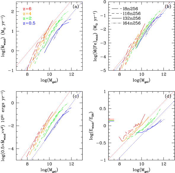
Figure 9: Feedback properties are shown as a function of galaxy mass (derived by SKID) for 4 redshifts for our $\sigma$-derived wind simulations at various box sizes. Red and blue dotted lines are our “toy models” calculated using momentum-driven wind relations and assuming specific star formation rates of 0.1 and 1.0 Gyr^-1, and metallicities of $Z=0.3Z_{\odot}$ and 1.0 for $z=6$ and 0.5 respectively. Mass and metal feedback (Panels (a) and (b)) are predicted to go as $M_{\rm gal}^{2/3}$, although metallicity feedback additionally depends on the gas mass-metallicity of galaxies, where $Z\propto M_{\rm gal}^{0.3}$. Energy feedback, in $10^{51}$ erg units (Panel (c)) follows the predicted $M_{\rm gal}^{4/3}$ relation very closely, and the ratio wind energy efficiency, $E_{\rm wind}/E_{\rm SN}$, (Panel (d)) rises nearly as $M_{\rm gal}^{1/3}$ for most redshifts. The lines on the left of Panel (d) show the average $E_{\rm wind}/E_{\rm SN}$ efficiency in the l32n256 box is declining slightly, although these values may be lower when lower mass galaxies not resolved in this box are included.

Figure 9 quantifies mass (upper left), metal (upper right) and energy (lower panels) feedback, as a function of galaxy mass in our $\sigma$-derived wind simulations at four chosen redshifts ($z=6,4,2,0.5$). We choose $z=0.5$ to represent the local Universe rather than $z=0$, because we want to follow the evolution of wind materials after they are launched and consider 5 Gyr a compromise as enough time for the winds cycle to play out, but not too much such that the cosmological evolution is overly significant. The upper left panel shows the mass loss rate in outflows as a function of galaxy baryonic mass. At a given galaxy mass, the outflow rate goes down with time, by roughly a factor of 10 from $z=6\rightarrow 0.5$. Remember that this is the rate of mass being driven from the galaxy’s star-forming region; whether the material makes it to the IGM or remains trapped within the galactic halo will be examined later.

Along with the results of our simulations, we plot two simple ”toy models” of feedback behavior corresponding to galaxies forming stars at constant specific star formation rates (i.e. star formation rate per unit stellar mass) of 1.0 and 0.1 Gyr^-1; these roughly correspond to typical star forming galaxies at $z=6$ and $z=0.5$ respectively. The momentum-driven wind model predicts that mass feedback should go as $\dot{M}_{\rm wind}\propto$ SFR$/\sigma\propto$ SFR$\times M_{\rm gal}^{-1/3}H(z)^{-1/3}$. Making the reasonable assumption that SFR$\propto M_{\rm gal}$ as typically found in simulations (e.g. , 2008), then this simple model would predict $\dot{M}_{\rm wind}\propto M_{\rm gal}^{2/3}H(z)^{-1/3}$. The dotted lines in Figure 9 show these relations for our toy models. The red dotted line fits well to $z=6$ at $M_{\rm gal}=10^{9.5-10}M_{\odot}$ showing these galaxies efficiently doubling their mass every 1.0 Gyr, while the doubling time is around 10 Gyr for galaxies at $z=0.5$.

The typical mass outflow rate reduces with time for two reasons: First, the star formation rates are lower owing to lower accretion rates from the IGM, as discussed in SH03b and OD06 and as observed by (2005, 2006, 2006). Second, galaxies grow larger with time and the mass loading factors drop; this even despite the $H(z)^{-1/3}$ factor that actually increases $\eta$ for a galaxy of the same mass at lower redshift. Hence the outflow rates qualitatively follow the trend seen in observations that at high redshifts, outflows are ubiquitous and strong, while at the present epoch it is rare to find galaxies that are expelling significant amounts of mass.

Figure 9, upper right panel, shows the mass of metals launched as wind particles, which is $\dot{M}(Z)_{\rm wind}\propto M_{\rm gal}^{2/3}H(z)^{-1/3}Z_{\rm gal}$. For concreteness we follow the iron mass, although other species show similar trends; recall that even at $z=0$ 93% of iron is produced in Type II SNe, and the fraction is higher at higher redshifts. This relation can be thought of as the $M_{\rm gal}-\dot{M}_{\rm wind}$ relation shown in the upper left panel convolved with the star formation-weighted gas mass-metallicity relations of galaxies at the chosen redshifts, since it is this gas that is being driven out in outflows. (2008) showed how our ’vzw’ model reproduces the slope and scatter of the mass-metallicity relationship of galaxies as observed by (2006) for $z=2$ Lyman break galaxies. Again, we plot two dotted lines corresponding to our toy models with a $Z\propto M_{\rm gal}^{0.3}$ dependence accounting for the mass-metallicity relationship normalized to $z=0.3$ and $1.0Z_{\odot}$ at $10^{11}M_{\odot}$ for $z=6.0$ and 0.5 respectively. The two toys models show little evolution (0.18 dex decline from $z=6\rightarrow 0.5$, because the declining $\dot{M}_{\rm wind}$ is counter-balanced by an increasing metallicity for a given mass galaxy toward lower redshift. In the l32n256vzw-$\sigma$ simulation, a $10^{10}M_{\odot}yr^{-1}$ galaxy injects $7.7\times 10^{-3}M_{\odot}yr^{-1}$ of iron at $z=6$ and $2.2\times 10^{-3}M_{\odot}yr^{-1}$ at $z=0.5$.

In the lower left panel we plot the total feedback energy per time (i.e. feedback power) imparted into wind particles as a function of galaxy mass. This power is $\dot{E}_{\rm wind}=0.5\dot{M}_{\rm wind}\times{v_{\rm wind}}^{2}\propto$ SFR$\times\sigma H(z)^{1/3}\propto M_{\rm gal}^{4/3}H(z)^{1/3}$, using the same assumption of SFR $\propto M_{\rm gal}$. The feedback power is shown in units of $10^{51}$ ergs yr^-1, which can be thought of as the number of SNe per year. Our simulations follow the trend of the toy models in terms of redshift evolution, and show an even tighter agreement at the low mass end versus $M_{\rm gal}$ than the mass feedback; the metallicity dependence gives greater energies to winds from lower mass, less metal-rich galaxies. Energy feedback is an even stronger function of galaxy mass than mass or metallicity feedback.

The bottom right panel in Figure 9 shows feedback energy relative to supernova energy ($E_{\rm wind}/E_{\rm SN}$). This quantity decreases with time, and increases with galaxy mass. The toy models shown represent $E_{\rm SN}\propto$ SFR $\propto M_{\rm gal}$, or $E_{\rm wind}/E_{\rm SN}\propto M_{\rm gal}^{1/3}H(z)^{1/3}$. At the low-mass end, the simulations rise above the toy model and show more scatter due to uncertainties in the the star formation rates of the smallest galaxies, but the slope at most redshifts is correct. At the high-mass end, momentum-driven wind energy exceed the supernova energy, which is physically allowed since the UV photons produced during the entire lifetimes of massive stars drive winds in this scenario (see OD06, Figure 4). Summing this ratio globally over all galaxies at each redshift, we obtain the values shown by the tick marks on the left side of the panel. Globally, the average $E_{\rm wind}/E_{\rm SN}$ ratio exceeds unity at all redshifts (being around 1.2), and is surprisingly constant, declining less than 0.1 dex from $z=6\rightarrow 0.5$ in the new $\sigma$-derived formulation of the winds. The decline of wind energy feedback for a given mass galaxy toward lower redshift is mostly counterbalanced by more massive galaxies driving more energetic winds at these redshifts. Less massive galaxies unresolved in the l32n256 box are likely to lower this value somewhat, so we only want to conclude that the wind energy is similar to the supernova energy and stays remarkably unchanged with redshift in the $\sigma$-derived momentum driven wind model.

To summarize, the momentum-driven wind simulations follow trends expected from the input momentum-driven outflow scalings. This is of course not surprising, and at one level this is merely a consistency check that the new wind prescription and the group finder are working correctly. But this also gives some intuition regarding outflow properties as a function of galaxy mass required to achieve the successes enjoyed by the momentum-driven wind scenario. For example, mass outflow rates should correlate with galaxy mass, and outflow energy in typical galaxies is comparable to, and perhaps exceeds, the total available supernova energy. These trends provide constraints on wind driving mechanisms and inputs to heuristic galaxy formation models such as semi-analytic models.

5.2 Feedback by Volume

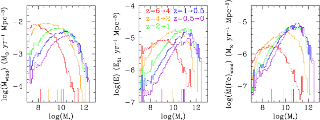
Figure 10: Mass, metallicity, and energy feedback per cubic Mpc binned by stellar mass (0.1 dex bins, derived by SKID) in 5 redshift bins covering $z=6\rightarrow 0$. Histograms include data from 8, 16, 32, and 64 $h^{-1}{\rm Mpc}$ in order to resolve a large range (5 decades) of galaxy masses. Vertical lines with colors corresponding to their redshift range show the median galaxy producing each type of feedback. For all forms of feedback, the median $M_{*}$ increases by a factor of 100 between $z=6\rightarrow 0$; most of this increase ($30\times$) is between $z=6\rightarrow 2$. However each form of feedback favors a different mass-scale: $10^{10.2}M_{\odot}$ for mass, $10^{11.0}M_{\odot}$ for energy, and $10^{10.7}M_{\odot}$ for metallicity. The mass resolution limits are $1.9\times 10^{7}M_{\odot}$ above $z=4$ and $1.5\times 10^{8}M_{\odot}$ below.

We shift from examining feedback trends in individual galaxies to studying feedback trends per unit volume. In order to facilitate observational comparisons, we use use stellar mass, $M_{*}$, rather than baryonic mass.

In Figure 10 we plot histograms binned in 0.1 dex intervals of the three forms of feedback at five redshift bins from $z=6\rightarrow 0$ parameterized by the amount of feedback per cubic Mpc. These histograms include all SKID-identified galaxies in the 8, 16, 32, and 64 $h^{-1}{\rm Mpc}$ boxes in order to obtain the large dynamical range covering over 5 decades of galaxy masses. The less computationally expensive l8n128vzw simulation was included in the histograms between $z=0-1.5$ to probe the least massive galaxies in this range, since the l16n256vzw run at the same resolution ends at $z=1.5$. We also plot the median $M_{*}$ of a galaxy contributing to each type of feedback shown as vertical lines at the bottom of each panel.

The mass, energy, and metal outflow rates peak at increasingly higher galaxy masses with time. The galaxy mass resolution limits are $1.9\times 10^{7}M_{\odot}$ at $z\geq 4$ and $1.5\times 10^{8}M_{\odot}$ below; the peaks are mostly comfortably above these resolution limits, indicating that we have the necessary resolution to resolve the source of feedback across our simulation boxes for the three forms of feedback. The exceptions are the mass outflow rates at $z>2$, which peak less than 1 dex from these limits. The changing resolution limit at $z=4$ raises concern whether the evolution above and below this limit is real; however, the larger amount of evolution between $z=4\rightarrow 1$, despite an unchanging resolution limit shows that evolution at $z<4$ is not just a resolution effect.

The median galaxy $M_{*}$ expelling gas increases by $\sim 100\times$ between $z=6\rightarrow 0$, for all three forms of feedback. The vast majority of this growth occurs between $z=6\rightarrow 2$, where the median stellar mass increases by $\sim 30\times$ in just 2.3 Gyr. This is the epoch of peak star formation in the Universe, so it is not surprising that galaxies show the most growth in their stellar masses then. The baryonic mass (stars plus gas, not shown) also jumps significantly, $\sim 10-15\times$, but early small galaxies are more gas rich making the jump less extreme. Nevertheless, the evolution is much slower in the 10 Gyr between $z=2\rightarrow 0$ as both median $M_{*}$ and $M_{\rm gal}$ at most triple and usually double in this longer timespan. This late growth could be an overestimate because of our overestimated star formation rates at late times in the most massive galaxies. It is quite possible that if our simulations could properly curtail massive galaxies from forming stars, median $M_{*}$ would fall toward $z=0$.

The same growth patterns for star formation-driven feedback are also seen in the median galaxy weighted by SFR, which itself is highly correlated with $M_{\rm gal}$ as (2008) shows using these same simulations. Therefore the changing mass scales of star formation-driven feedback reflect the hierarchical growth of galaxies between $z=6\rightarrow 0$, with most growth occurring before $z=2$.

While it is no coincidence that all three forms of feedback show similar growth rates in median $M_{*}$ (and $M_{\rm gal}$), each feedback form has a different mass preference and peaks at a different epoch. Mass feedback preferentially traces smaller galaxies due to the inverse relationship of $\eta$ with $M_{\rm gal}$. High mass loading factors from small galaxies, which dominate star formation at high redshift are necessary to curtail the star formation density at early times (OD06) and fit galaxy luminosity functions at $z>3$ (, 2006, 2007). The mass feedback density peaks at $z\sim 3.5$ at $0.28M_{\odot}yr^{-1}{\rm Mpc}^{-3}$. The median galaxy in the relatively nearby Universe bin ($z=0.5\rightarrow 0$) has $M_{*}=10^{10.2}M_{\odot}$, or 1/6th the (2003) $M^{*}$ value of $10^{11.0}M_{\odot}$ in stellar mass.

The median $M_{*}$ for energy feedback is biased toward larger galaxies for momentum-driven winds. Our simulations suggest that the median galaxy adding energy to the IGM is an $M^{*}$ galaxy ($M_{*}=10^{11}M_{\odot}$) in the local Universe. Observations disagree with this prediction, since the prototypical local galaxy exhibiting feedback is more like M82, an $\sim 0.1M^{*}$ galaxy. Moreover most super-$M^{*}$ galaxies are red and dead, unable to generate star formation-driven winds. This again suggests that a more realistic truncation of star formation in low-$z$ massive galaxies could alter the exact values quoted here. However, at high-$z$ where the typical galaxy appears to be driving an outflow (, 2006), these results should be more robust. The energy feedback density peaks at $z\sim 2.5$ at an equivalent energy of $5\times 10^{-4}$ SN yr^-1 Mpc^-3 ($10^{51}$ ergs each).

The metallicity feedback grows the fastest of all forms of feedback during the epoch of peak star formation, and does not obtain its maximum density until slightly past $z=1$ ($\dot{M}(Fe)_{\rm wind}=1.7\times 10^{-4}M_{\odot}$ yr^-1 Mpc^-3). The metallicity feedback is simply the mass feedback modified by the mass-metallicity relationship of galaxies, which favors higher $M_{*}$ and lower redshift. The median $M_{*}$ at $z=0$ is $0.5M^{*}$, or $\sim 5\times$ higher than the $0.1L^{*}$ median galaxy as determined by B07. However, we do not think that this is an inconsistency due to an overestimate in massive galaxy star formation at low redshift, but instead a result of measuring different quantities. We are measuring the amount of feedback leaving a galaxy’s star forming region whereas B07 measures the feedback expelled from the galaxy reaching the IGM by determining the effective yield as a function of $v_{\rm rot}$ . As we will show next, much of the mass and metals that are expelled never leave their parent haloes and are reaccreted in a timescale often much less than the Hubble time. The leads us to introduce the important concept of wind recycling.

5.3 Wind Recycling

What happens to the mass and metals once they are expelled from the galaxies’ star forming regions? Is all feedback best described as galactic superwinds or does some feedback never really escape from its parent halo and should more accurately be considered a halo fountain? To answer such questions we introduce the concept of wind recycling, which plays an important role in feedback over cosmic time.

By following wind particles by their particle IDs during the simulation run, we can track how many times the same SPH particle is recycled in a wind. For the l32n256vzw-$\sigma$ simulation evolved all the way to $z=0$ we find that a wind particle is launched an average of 2.5 times; while 18.3% of SPH particles are ever launched in a wind, the summed number of wind launches equals 45.7% of the total number of SPH particles. Wind recycling dominates over winds being launched from galaxies for the first time– the average wind particle across time is more likely to have already been launched in a wind! The most important aspect is that wind material, once launched, cannot be assumed to be lost from the galaxy forever and remaining in the IGM. This is true despite the fact that, in our momentum-driven wind prescription, outflows are always ejected at speeds exceeding the escape velocity of its parent galaxy. Gravitational infall and hydrodynamic effects both conspire to slow down outflows and facilitate wind recycling.

Figure 11 displays histograms of the number of times the same wind particle is recycled, $N_{\rm rec}$, in the l32n256 simulation. Only 17% of all winds are particles ejected one time and therefore never recycled (i.e. $N_{\rm rec}=0$); this corresponds to 7.9% of all SPH particles. The record-holder is a particle recycled an astonishing 30 times indicating that probably in this case the term halo fountain may be more appropriate than galactic superwind. Perhaps the most telling statistic is half of the wind particles have been recycled 3 or more times. The continuous range in the number of recycling times blurs the distinction between a galactic superwind and a halo fountain, and suggests instead there is a continuum.

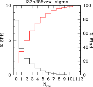
Figure 11: The percentage of all SPH particles recycled $N_{\rm rec}$ times by $z=0$ in the $32h^{-1}{\rm Mpc}$ $2\times 256^{3}$ simulation is shown by the black histogram (left scale). $N_{\rm rec}=0$ means a wind particle is launched only once. The red line shows the cumulative sum of wind particles launched per bin (right scale, normalized to 100%) and is the sum of $(N_{\rm rec}+1)$ multiplied by the black histogram added left to right. 50% of winds are particles that have been or will be recycled 3 or more times indicating that wind recycling plays a significant if not dominant role in feedback.

The concept of recycling is not unexpected, and has been predicted by (, 2007) from semi-analytical models. DO07 showed that metals move from mean cosmic density at $z=2$ to an overdensity of 100 by $z=0$ as baryons migrate into larger structures as part of cosmic structural growth. This means that most of the metals in the diffuse IGM at $z\sim 2$ are in galactic haloes at $z\sim 0$. Metals blown out from early galaxies to low overdensities are later reaccreted in the formation of larger structures, and blown out again. Still, the commonality of wind particles being recycled is surprising, especially since momentum-driven winds are almost always ejected at velocities well in excess of the escape velocity of the galaxy. It is in fact more appropriate to talk about how long it takes a wind particle to be recycled instead of whether it will be recycled. Metals injected by galactic superwinds cannot be assumed to remain permanently in the IGM; metals continuously cycle between galaxies and the IGM. In an upcoming paper we will quantify the ages of metals observed at different absorption lines tracing different regions of the IGM. For now we note that the average ages of the metals in the IGM are typically much shorter than the age of the Universe.

Do wind particles generally return to their parent galaxy, or do they jump from galaxy to galaxy? The answer is the former; in the vast majority of cases a wind particle returns to either its parent galaxy or the result of a merger involving the parent galaxy. 95% of recycled wind particles are re-launched from a galaxy of similar or more mass than the previous recycling. Of course galaxies grow anyway under the hierarchical growth scenario, so a wind particle could join a different galaxy that has itself grown larger than its parent. By considering wind particles recycled within 10% of the Hubble time, we can diminish the bias of galaxy growth and explore whether winds are traveling from massive central galaxies to surrounding satellite galaxies possibly affecting their dynamics and enrichment histories. With this time limit, 97% of winds return to more massive galaxies indicating this is a less likely trend. The number jumps to 99% when considering winds launched from $M_{\rm gal}>10^{11}M_{\odot}$, indicating that it is harder to escape from a more massive galaxy. Furthermore, a wind particle is rarely relaunched more than 1 comoving $h^{-1}{\rm Mpc}$ apart in a 16 $h^{-1}{\rm Mpc}$ test simulation; the minority case usually involves wind particles following the position of a fast moving parent galaxy. Winds rarely escape forever their parent halo, and winds from large central galaxies do not appear to disrupt satellite galaxies.

Another way to quantify wind recycling is using the summed amount of material injected into winds. We introduce the quantity $\Omega_{\rm wind}$, which is the mass injected in winds, including recycled gas. Owing to recycling, there is no limit to how large this can be. Using our l32n256 run, we find that $\Omega_{\rm wind}=0.39\Omega_{b}$– i.e. an equivalent of 39% of the baryonic mass has been blown out in a galactic superwind by $z=0$. This is significantly larger than $\Omega_{*}=0.097$ due to mass loading factors greater than one as well as recycling.

The other $\sigma$-derived wind runs to $z=0$ give different values: $\Omega_{\rm wind}=0.59\Omega_{b}$ for the 8 $h^{-1}{\rm Mpc}$ box with $128^{3}$ SPH particles, and $\Omega_{\rm wind}=0.23\Omega_{b}$ for the 32 $h^{-1}{\rm Mpc}$ box also with $128^{3}$ particles. $\Omega_{\rm wind}$ increases by 160% when mass resolution changes by $64\times$. This jump is primarily due to a 70% increase in $\Omega_{*}$, but still leaves another 50% likely due the varying treatment of recycling at different resolutions. This lack of resolution convergence raises the question of whether the amount of recycling is set by numerics, perhaps arising from the poor treatment of SPH trying to model outflow processes occurring at resolutions below the limit of our simulations.

The discontinuity in recycling rates between resolutions stems from how long and how far a particle reaches once it has been launched. Wind particles in the 32 $h^{-1}{\rm Mpc}$ $2\times 256^{3}$ box with typical masses of $3.2\times 10^{7}M_{\odot}$ are shot at hundreds of $\;{\rm km}\,{\rm s}^{-1}$– a huge bundle that may be more accurately thought of as a flying wind “bullet”. An actual wind should form a bow shock resulting in a plume of material spreading laterally, but instead in SPH this speeding bullet is slowed down viscously through the interactions with neighboring particles. The number of interacting neighbors over the same physical distance is lower at less resolution, and a wind particle will take longer to slow down; this is an unfortunate but unavoidable consequence of SPH. Hence lower resolution simulations inhibit recycling as evidenced by the average number of times an individual wind particle is launched: 3.0, 2.5, and 2.1 times for 4.7, 38, and 300$\times 10^{6}M_{\odot}$ SPH particle resolution (to $z=0$). This lack of resolution convergence is quantifiable by the median recycling timescale of wind particles in different resolution simulations as shown in the upper right panel of Figure 12, and is discussed in the following subsection. Increased resolution suggests that wind recycling should move $\Omega_{\rm wind}$ to an even higher value, probably exceeding $1/2\Omega_{b}$. Given that galaxies below a certain mass cannot form owing to the presence of an ionizing background, there will be a limit to how high $\Omega_{\rm wind}$ can be; in the future we hope to run simulations that can achieve such resolutions in a cosmologically representative volume. For now, the wind recycling predictions should be considered as illustrative rather than quantitative.

5.4 Wind Recycling Timescales

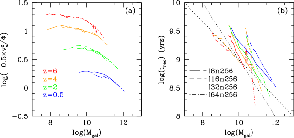
Figure 12: The virial ratio ($E_{\rm rat}$, the ratio of wind kinetic energy to potential well energy) are displayed as a function of galaxy mass (derived by SKID) at 4 launch redshifts in Panel (a) for our $\sigma$-derived wind simulations at various box sizes. The shallow turnover at high-mass is mostly due to imposed wind speed limits. Panel (b) shows that the recycling timescale (the median time for a wind particle to be relaunched in a wind) is a much stronger function of $M_{\rm gal}$. After exploring alternatives for the $M_{\rm gal}-t_{\rm rec}$ anti-correlation, we conclude winds from more massive galaxies encounter a denser environment slowing the wind particle faster and allowing it to be re-accreted faster. The two dotted lines show the galaxy mass dependence of $t_{\rm rec}$ is dominated by slowing due to environment, $M_{\rm gal}^{-1/3}$, or the gravitational free-fall time, $M_{\rm gal}^{-1/2}$; wind particles spend most of their time falling back into a galaxy. The poor resolution convergence in $t_{\rm rec}$ indicates lower resolution simulations overpredict the $t_{\rm rec}$ and underpredict the total amount of wind recycling. To see wind recycling in action in our simulations, see the movies and an explanation at http://luca.as.arizona.edu/~oppen/IGM/recycling.html.

We now examine wind recycling as a function of galaxy mass. Specifically, we want to know what galaxies are able to inject their metals into the IGM. The common thought is that low-mass galaxies lose their metals more easily because winds can escape from these galaxies’ shallower potential wells (e.g. , 1986). As (2003) showed, if the outflow energy couples efficiently to ambient halo gas, this can yield the mass-metallicity relation as observed, as well as other properties of dwarf galaxies. However, (2008) showed that a model in which galaxies expel material at constant velocity (i.e. the “constant wind” model of OD06) does not reproduce the observed mass-metallicity relation, primarily because outflows do not in fact couple their energy efficiently to ambient gas. Instead, the observed mass-metallicity relation (e.g. , 2006, 2004) are better reproduced in the momentum-driven wind scenario. In this case, since ${v_{\rm wind}}\propto\sqrt{-\Phi_{\rm gal}}$ (roughly), all outflows have an approximately equal probability of escaping their parent haloes independent of mass, when considering only gravitational interactions with an isolated halo.

The left panel of Figure 12 shows the virial ratio, $E_{\rm rat}\equiv 0.5{v_{\rm wind}}^{2}/\Phi$, as a function of galaxy baryonic mass, for winds launched at four redshifts. At any given redshift, the ratio is roughly constant, but rises slightly at low masses and then declines to higher masses. At low masses, the trend arises from the mild metallicity dependence of ${v_{\rm wind}}$ together with the mass-metallicity relation. Moving to higher masses, since the potential $\Phi$ includes the galaxy potential and the environmental potential of the group/cluster in which it lies, and since massive galaxies live in denser environments, $\Phi$ is greater. At the highest masses, our imposed speed limit reflecting the assumption that wind energy cannot exceed twice the supernova energy reduces wind velocities. Note that by definition, $\Phi$-derived winds will have a constant $E_{\rm rat}$ for a given launch redshift (modulo wind speed limits); hence the curvature towards high masses is predominantly a reflection of $\sigma$-derived winds.

In practice, outflows are not only confined by the gravitational potential of the host galaxy; cosmic infall and hydrodynamic effects can also be quite important. For instance, (2005) used a simulation of a typical LBG at $z=3$ ($M_{\rm dyn}=2\times 10^{11}M_{\odot}$) to show that metals never reach the IGM and instead are confined to the surrounding hot halo gas by infalling gas that creates a shock interface with the outflow.

One way to quantify such additional effects is to consider a new timescale called the recycling timescale, $t_{\rm rec}$, which is defined as the median time for a wind particle to be re-ejected again as a wind particle, or else fully converted into a star. At all launch redshifts explored, for all $M_{\rm gal}$, more than half of wind particles recycle meaning that $t_{\rm rec}$ can be measured. The right panel of Figure 12 shows $t_{\rm rec}-M_{\rm gal}$ relation, demonstrating a strong anti-correlation of $t_{\rm rec}$ with galaxy mass. The simple fact that winds recycle on short timescales even though they are launched at velocities well above the escape velocity is an indication that slowing by ambient gas and surrounding potentials is significant.

If the galaxy’s gravity is dominant in confining its outflow, one would expect that the time spent away from the galaxy would be approximated by twice the free-fall timescale, $t_{\rm ff}$ (one $t_{\rm ff}$ outward and another one back in, or simply the orbital timescale for an orbit of eccentricity 1). $t_{\rm ff}$ scales as $R_{\rm turn}^{3/2}M_{\rm dyn}^{-1/2}$, where $R_{\rm turn}$ is the turn-around distance of the wind particle, and $M_{\rm dyn}$ is the dynamical mass of the galaxy treated as a point source for the sake of simplicity. Following Newtonian dynamics, $R_{\rm turn}\propto M_{\rm dyn}/{v_{\rm wind}}^{2}$, and the ${v_{\rm wind}}\propto M_{\rm gal}^{1/3}$ relation for momentum-driven winds, $t_{\rm ff}$ remains invariant as a function of galaxy mass while $R_{\rm turn}\propto M^{1/3}$. Momentum-driven winds should reach a maximum distance from their parent galaxy that is a constant multiple of the virial radius since ${v_{\rm wind}}$ scales with the virial energy of an isolated halo. The strong trend of $t_{\rm rec}$ with $M_{\rm gal}$ indicates that larger-scale potentials and hydrodynamic effects are dominant.

Is the particle spending more time in the IGM/galactic halo or in the galactic ISM before being relaunched? The answer is that the vast majority of the time between recycling is spent outside the star forming regions of a galaxy. This is not surprising, because in our simulations the star formation timescale is tied completely to the accretion timescale; once a particle is in a galaxy it gets converted to a star or blown out in a wind much more quickly than it was accreted (, 2008). Therefore, we subdivide $t_{\rm rec}$ into two timescales, one leaving the galaxy to reach $R_{\rm turn}$ while being slowed by hydrodynamical forces, $t_{\rm out}$ and the other returning to the galaxy in approximately one $t_{\rm ff}$. For simplicity, let’s say the hydrodynamic forces slow the wind particle down at a constant rate, in which case $t_{\rm out}=R_{\rm turn}/({v_{\rm wind}}/2)$. The total recycling timescale can be approximated as

$$\frac{t_{\rm rec}}{1\rm{Gyr}}=1.96\left(\frac{R_{\rm turn}}{100\rm{kpc}}\right)\left(\frac{100\;{\rm km}\,{\rm s}^{-1}}{{v_{\rm wind}}}\right)$$

$$+~{}2.09\left(\frac{R_{\rm turn}}{100\rm{kpc}}\right)^{3/2}\left(\frac{10^{10}M_{\odot}}{M_{\rm gal}}\right)^{1/2}$$ (9)

if we assume that $M_{\rm dyn}=\Omega_{M}/\Omega_{b}\times M_{\rm gal}$ and $R_{\rm turn}$ is in physical kpc. We can now solve for $R_{\rm turn}$ by taking the $t_{\rm rec}$ from Figure 12 and the average ${v_{\rm wind}}$ from Figure 3. $R_{\rm turn}$ is just an upper limit for how far wind particles with median $t_{\rm rec}$ can extend from a parent galaxy, because in reality a particle does not likely go out and then immediately fall back into a galaxy in two steps; wind particles often spend time orbiting around their parent galaxies as well.

In principle, $R_{\rm turn}$ can be tracked directly in simulations, however our current suite of runs did not output position information of wind particles owing to the large storage requirements. We have checked for isolated cases that our simple formula (eq. 5.4) yields roughly correct results.

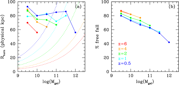
Figure 13: Panel (a) shows $R_{\rm turn}$, the maximum radial extent a median wind particle may extend from its parent galaxy calculated from equation 5.4 in the l32n256 simulation. $R_{\rm turn}$ generally is larger at smaller $M_{\rm gal}$; this trend coupled with the fact that $t_{\rm rec}$ is longer indicates that smaller galaxies can more easily enrich the IGM. Dotted lines corresponding to a NFW halo radius, $r_{\rm 200}$ (1997), show that winds from $L^{*}$ galaxies do not escape their parent haloes at $z<1$. Panel (b) shows that winds from small galaxies spend more time on their journey returning to a galaxy than being blown out.

We plot $R_{\rm turn}$ in the left of Figure 13, focusing first on the trend over 2.5 decades of galaxy masses at $z=0.5$, which we consider here the local Universe since trends do not evolve much until $z=0$. $R_{\rm turn}$ stays nearly constant from the size scale of dwarf galaxies to galaxies above $L^{*}$ while $t_{\rm rec}$ declines. Dotted lines correspond to the radius, $r_{\rm 200}$, of a NFW halo (, 1997). The point at which $R_{\rm turn}$ and $r_{\rm 200}$ intersect is the approximate transition mass below which winds reach the IGM and above which winds are confined to their haloes. Metals rarely enter the IGM from galaxies above $10^{11}M_{\odot}$ in the local Universe. Several significant conclusions can be drawn from this behavior at low-$z$.

First let us consider our wind model and the Milky Way, which has $M_{\rm gal}\sim 10^{11}M_{\odot}$. Our wind model produces an outflow from a Milky Way-type galaxy, with initial speeds of a few hundred $\;{\rm km}\,{\rm s}^{-1}$. One might claim that this immediately invalidates our model, since the Milky Way is not observed to have an outflow. Yet quantitatively, our model predicts that a Milky Way-sized galaxy should have a recycling time of less than 1 Gyr, and the typical wind particle will not venture beyond 85 kpc (if we assume not much has changed between $z=0.5\rightarrow 0$). In other words, in our model, the Milky Way is not driving a classical outflow as seen from local starbursts, but rather is continually sending material up into the halo and having it rain back down on a timescale of 1 Gyr. We call this a halo fountain, in analogy with a galactic fountain that operates on smaller scales. Indeed, we speculate that there may not be a fundamental difference between galactic fountains and halo fountains, but rather gas is being thrown out of the disk at a range of velocities; however, our simulations lack the resolution to address this issue directly.

How might such a halo fountain be observed? One possibility is that it has already been seen, as high velocity clouds (HVC’s). (1997) predict that given the observed rate of material going into HVC’s of about 5 $M_{\odot}yr^{-1}$ then it should take $\sim 1$ Gyr for all the gas in the ISM to cycle through this halo fountain. Hence the Galaxy may have an active halo fountain recycling its material on a timescale much less than a Hubble time, despite not resembling anything like a starburst galaxy. The difficulty of observation of feedback within our own Galaxy may just indicate how invisible yet ubiquitous galactic-scale winds are.

Secondly, with $R_{\rm turn}$ nearly constant, $t_{\rm rec}$ should be proportional to $M_{\rm gal}^{-1/3}$ if dominated by $t_{\rm out}$ and $M_{\rm gal}^{-1/2}$ if $t_{\rm ff}$ is larger. The black dotted line in the right of Figure 12 corresponding to the latter case (the steeper of the two) appears to more closely match the general trends indicating that $t_{\rm ff}$ dominates; wind particles spend a majority of $t_{\rm rec}$ falling into galaxies (Panel (b) in Figure 13). Our calculations above agree $t_{\rm ff}$ grows larger than $t_{\rm out}$ for smaller galaxies, but the two timescales are similar for extremely massive galaxies, $M_{\rm gal}\sim 10^{12}M_{\odot}$.

Thirdly, smaller galaxies live in less dense environments where hydrodynamic slowing takes longer. To demonstrate this we look at another parameter, the minimum overdensity reached by wind particles, which should approximately correspond to the density at $R_{\rm turn}$. For the subset of wind particles we track the minimum density achieved before recycling, $\rho_{\rm min}$. Figure 14 (solid lines) shows the median $\rho_{\rm min}$ as a function of the baryonic mass of the originating galaxy, $M_{\rm gal}$, from the l32n256 run. At all redshifts, smaller galaxies push their winds to lower densities, consistent with them having longer recycling times. Their less dense environments slow winds over a longer $t_{\rm out}$, and allow them to reach a similar $R_{\rm turn}$ as more massive galaxies despite lower ${v_{\rm wind}}$. We also plot a long-dashed line that show the average density within 1 comoving Mpc sphere around the $z=0.5$ galaxies. These show a similar trend, indicating that environmental dependence is the primary factor in how far winds reach into the IGM and how long they remain there. The fact that $\rho_{\rm min}$ is much higher than the density within 1 Mpc is an indication that these winds are traveling much less than that distance as our calculations above indicate ($\sim 80$ kpc comoving at $z=0.5$).

Although a possible explanation for the trend in $\rho_{\rm min}$ is larger haloes have higher densities at the same distance, this cannot account for the dependence. The density of NFW haloes decline nearly as $1/r$ beyond $r_{200}$ resulting in a $\rho_{\rm min}\propto M_{gal}$ dependence much steeper than plotted in Figure 14 below $z=2$; for all but the most massive galaxies the density contribution of the parent halo is much smaller at $\rho_{\rm min}$. The flattening of this relation toward $z=0$ at $M_{gal}<10^{11}M_{\odot}$ means these galaxies more likely live in denser environments. For more massive galaxies, the parent halo itself is more responsible for the hydrodynamical slowing.

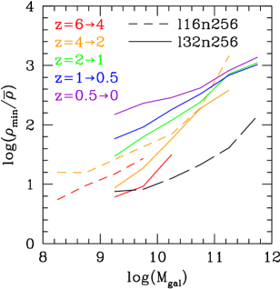
Figure 14: The minimum density a wind particle achieves between recyclings is shown to be a strong function of galaxy mass at all redshifts (colored lines). Lower mass galaxies have longer recycling times, because winds are launched into less dense environments where shocks take longer to slow and turn around winds. The environmental density within sphere of 1 comoving Mpc as a function of $M_{\rm gal}$ at $z=0.5$ (black dashed line from l32n256 simulation) shows the same trend as $\rho_{\rm min}/\bar{\rho}$ indicating that environment is the primary factor in how far winds reach into the IGM. The NFW halo profile alone cannot explain this trend as halo profiles drop much more sharply and the environmental density dominates for all but the most massive galaxies at low-$z$.

Finally, small galaxies can enrich a similar volume as large galaxies leading to major implications as to which galaxies enrich the IGM. Metals from small galaxies have the advantage of staying in the IGM longer, however the disadvantage of their winds being less metal enriched (e.g. Panel (b) of Figure 9). We plan to look at the origin of IGM metal absorbers in a future paper, exploring what galaxies enrich the IGM, how long these metals have been in the IGM, and what distance metals travel from their parent galaxy.

As a side note, we admit that the global SFRD is overestimated at late times ($z<0.5$); the l32n256 run showing nearly 4$\times$ as much SF at $z=0$ relative to observations (Figure 4). The primary reason for this discrepancy is the lack of a quenching mechanism in the largest galaxies; galaxies above $10^{11}M_{\odot}$ account for 54% of star formation at $z=0$, and their continued late growth creates far too many galaxies above this mass as compared to observations (, 2008). The influence of these over-massive galaxies on the IGM however appears to be remote due to their inability to inject metals beyond their haloes and their short recycling timescales.

Turning to the evolution of recycling, $t_{\rm rec}$ grows moderately longer at lower redshift for a given $M_{\rm gal}$. For a $10^{10}M_{\odot}$ galaxy, $t_{\rm rec}$ is 1.1, 1.5, 1.6, and 2.0 Gyr for launch redshifts 6, 4, 2, and 0.5 respectively in the 32 $h^{-1}{\rm Mpc}$ box. This trend is in place despite $E_{\rm rat}$ declining by 1 decade from $z=6\rightarrow 0.5$ (see Figure 12(a)); wind kinetic energy is declining relative to the potential at their launch location. Again, the overriding variable is the slowing of the wind by the environment; the average physical density declines by a factor of 100 in this interval, making it easier for winds to travel further despite a factor of $10\times$ less energy input into the winds. Galaxies of the same mass are more likely to live at higher overdensities at lower redshift as structural growth makes more groups and clusters, but the declining physical densities and slower Hubble expansion of the Universe toward low redshift outweigh this.

While the $t_{\rm rec}$ grows at low redshift, the amount of the Universe it enriches sharply declines. The calculations of $R_{\rm turn}$ for equation 5.4 shows a moderately increasing physical distance from $z=6\rightarrow 0.5$ with values of 56, 71, 75, and 80 kpc for the four respective launch redshifts when considering the same $10^{10}M_{\odot}$ galaxy. However, the comoving volume such a galaxy is enriching is 35$\times$ greater at $z=6$ than at $z=0.5$. Momentum-driven winds can more easily expel metals into the IGM at high redshift, whereas the overdense environments combined with weaker wind velocities and the overall larger scale of the Universe leave metals perpetually recycling in halo fountains in groups and clusters at low redshift. These are the primary reasons metals migrate from the IGM to galaxies as the Universe evolves.

Our results compare favorably to those of (2007), who follow energy-driven winds ($\eta\propto\sigma^{-2}$ and ${v_{\rm wind}}\propto\sigma$) in their semi-analytical implementation using a two-phase process for the dynamical wind evolution (see also (2007)). At $z=0$ they also find that it is the smaller galaxies ($10^{10.5}M_{\odot}<M_{\rm dyn}<10^{11.5}M_{\odot}$, i.e. $\sim 1/10M^{*}$) that most efficiently inject their metals into the IGM ($\sim 40$% of the time), while metals from more massive haloes than $10^{12}M_{\odot}$ rarely escape the halo and are recycled (see their Figure 9). This is despite their ${v_{\rm wind}}$-dependence (same as ours but without the scatter) exceeding the escape velocity. The redshift dependence is harder to compare to our results due to differing definitions of escaped fractions into the IGM, but they do also see smaller haloes, the progenitors to massive galaxies today, as the most efficient enrichers of the IGM up to $z=4.5$.

Lastly, $t_{\rm rec}$ and $\rho_{\rm min}$ show similar resolution convergence issues as $\Omega_{\rm wind}$, for similar reasons. Lines at the same redshift do not overlap in either of these plots, indicating the $t_{\rm rec}$ is longer for the same $M_{\rm gal}$ at lower resolution. As discussed before, coarser resolution simulations slows down particles over a longer physical distance allowing wind particles to travel artificially too far at low resolution; this is why there is less recycling at lower resolution. For well-resolved galaxies, the lines of different resolution appear to nearly converge. The hydrodynamical treatment of wind particles after they are launched is not nearly as resolution-converged as the feedback properties on per galaxy basis (see Figure 9). Recycling times are overestimated when under-resolved. Hence recycling times may actually be shorter than we’ve shown.

In summary, we have shown that wind recycling is an important phenomenon for understanding the evolution of galaxies and the IGM. Winds from galaxies are typically expelled and re-accreted on timescales short compared to a Hubble time. This occurs despite the fact that winds are typically launched with plenty of kinetic energy to escape its halo. Such gravitational arguments are therefore not very relevant to understand how material cycles through galaxies and the IGM; instead, infall and shocks generated by outflows are more important in setting the wind distribution length- and time-scales. The recycling time is therefore strongly anti-correlated with galaxy mass, owing to the fact that more massive galaxies live in denser environments. These denser environments make it harder for winds to travel beyond their parent halo at late times causing the migration of metals from the IGM to galaxies from $z=2\rightarrow 0$. At the present epoch, small galaxies can still expel material, but larger galaxies are more aptly described as having halo fountains, in which material is constantly kicked up into the halo before raining down.

6 Summary

We introduce a new version of Gadget-2, with improvements designed to explore mass, metal, and energy feedback from galactic outflows across all cosmic epochs. We add two major modules designed to make the code better suited to explore the low-$z$ Universe: (1) A sophisticated enrichment model tracking four elements individually from Type II SNe, Type Ia SNe, and AGB stars; and (2) an on-the-fly galaxy finder used to derive momentum-driven wind parameters based on a galaxy’s mass.

We first run test simulations to explore global energy and enrichment properties with and without AGB and Type Ia feedback, and with our old and new wind implementations. Focusing on our new (galaxy mass-derived) winds including all sources of feedback, we then run several 34 million-particle simulations to explore feedback over the history of the Universe and over a large dynamic range in galaxy mass. We also track a representative subset of wind particles to study in detail how mass, metals, and energy are distributed by outflows.

Our new chemical enrichment model enables us to investigate the global production and distribution of key individual metal species. Globally, metal production of all four species tracked (C, O, Si, Fe) is dominated by Type II SNe at all redshifts. Type Ia SNe add significantly to the iron content of hot, intracluster gas, especially at $z<1$. AGB stars add moderately to the IGM carbon abundance by $z=0$, and provide fresh (enriched) gas for recycling into stars which increases global star formation at later epochs. Carbon yields from AGB stars cannot be ignored even at high-$z$, because carbon AGB stars enrich on timescales much less than a local Hubble time (i.e. 200 Myr-1 Gyr). Due to the complex interplay between instantaneous and delayed recycling from various forms, metallicity patterns in the IGM and ICM cannot be straightforwardly used to infer the enrichment patterns in the host galaxies responsible for polluting intergalactic gas.

We study enrichment patterns subdivided by baryonic phase. The total metal mass density is split roughly equally between galaxies and the IGM from $z=6\rightarrow 2$. Shocked intergalactic gas (WHIM and ICM) contains a fairly small portion of the global metal mass at all epochs. At $z<2$, metals tend to migrate from the IGM into galaxies, so that by $z=0$ about two-thirds of the metals are in galaxies (i.e. stars and cold gas). The combination of increased carbon and gas recycling from AGB feedback results in the IGM being significantly more carbon-enriched, which helps reproduce the relatively high observed mass density in C iv absorption systems at $z\approx 0$.

Our new galaxy mass-based wind model implementation provides a more faithful representation of the momentum-driven wind model of (2005), and yields outflows that are in better broad agreement with observed outflows. In particular, our implementation results in faster winds at high-$z$ and slower wind speeds at low-$z$ compared to our old local potential-derived winds. The fast early winds are able to enrich the IGM at early times as observed, while the slow late winds mean that most galaxies today are not driving material into the IGM at all. Qualitatively, this better agrees with observations indicating that most galaxies at $z\sim 2-3$ drive powerful winds (, 2006), while today galaxies are rarely seen to have strong outflows.

We examine bulk properties of outflows as a function of galaxy mass. We find that mass, metallicity, and energy feedback as a function of galaxy baryonic mass roughly follow the trends predicted by momentum-driven winds: $\dot{M}_{\rm wind}\propto M_{\rm gal}^{2/3}H^{-1/3}(z)$ and $\dot{E}_{\rm wind}\propto M_{\rm gal}^{4/3}H^{1/3}(z)$. The metal outflow rate is $\dot{M}_{\rm wind}Z_{\rm gal}$, where $Z_{\rm gal}\propto M_{\rm gal}^{1/3}$ with a proportionality constant that increases with time as given by mass-metallicity evolution (cf. , 2008). The stellar mass of the typical (median) galaxy most responsible for each particular form of feedback increases by a factor of $\sim 30$ between $z=6\rightarrow 2$, but only $\sim\times 2-3$ from $z=2\rightarrow 0$. Each form of feedback traces a different mass scale: mass feedback $\sim\frac{1}{6}M^{*}$, energy feedback $\sim M^{*}$, and metallicity feedback $\sim\frac{1}{2}M^{*}$. Measuring these characteristic masses (e.g. , 2007) offers the possibility to test whether momentum-driven wind scalings are followed globally.

The wind energy relative to the supernova energy scales roughly as $M_{\rm gal}^{1/3}$, and is within a factor of a few of unity at all epochs and galaxy masses. Given expected radiative losses from SN heat input into the ISM, it seems that SNe will have a difficult time providing enough energy to pollute the Universe as observed. An alternate source of energy would ease this tension, such as photons from young stars whose total energy can exceed the supernova energy by several orders of magnitude. This adds to the circumstantial evidence supporting the idea that galactic outflows may be driven in large part by radiation pressure, as postulated in the momentum-driven wind model.

We find that wind recycling, material ejected as outflows and then re-accreted and ejected again, turns out to be a remarkably common occurrence with significant dynamical repercussions. By following individual wind particles in our simulations down to $z=0$, we find that multiple recyclings are the norm, and that the typical wind particle has been ejected three to four times. In other words, outflow material being reaccreted onto a galaxy dominates over outflow material launched into the IGM forever. Since in our wind model all outflows are launched at speeds well above the escape velocity of galaxies, this indicates that outflows are mainly slowed through hydrodynamic interactions, allowing them to rejoin the hierarchical accretion flow into galaxies. Approximately 20% of the baryons participate in an outflow, but owing to multiple launchings the aggregate mass of baryons ejected exceeds half of the total baryonic mass. The two key corollaries of wind recycling as seen in our simulations are: (1) Material driven in an outflow cannot be assumed to remain in the IGM forever, and (2) Gravitational energetic considerations are generally not relevant for determining how far outflow propagate into the IGM.

We examine wind recycling as a function of galaxy mass. The recycling time scales roughly as $t_{\rm rec}\propto M_{\rm gal}^{-1/2}$, as expected if environmental effects are dominating the retardation of outflows. Larger galaxies have shorter recycling times despite launching winds at larger speeds, because they live in denser environments; the minimum overdensity achieved by winds scales with galaxy mass. As expected from the ubiquity of multiple recyclings, the recycling time is generally fairly short, roughly $10^{9\pm 0.5}$ years, increasing only mildly at lower redshift. Our analysis suggest that winds generally return to the galaxy from which they were launched (or its descendant), though a full merger tree construction is required to confirm this.

It is possible to estimate how far outflows travel from their host galaxies ($R_{\rm turn}$), as a function of galaxy mass and redshift. Remarkably, $R_{\rm turn}=80\pm 20$ physical kpc at all redshifts and masses. There are weak trends for higher $R_{\rm turn}$ at smaller masses and lower redshifts; both are consistent with ambient density being a key determinant for how far winds travel. The constant physical distance means that outflows at early epochs are able to enrich a significant fraction of the Universe, while outflows at later epochs are more confined around galaxies. This is the reason metals migrate from the IGM to galaxies between $z=2\rightarrow 0$.

Comparing $R_{\rm turn}$ to halo radii, we see that at $z>2$, typical $L^{*}$-sized galaxies have outflows that escape their host halos into the IGM, while at $z<1$ outflows are generally confined within galactic halos. This gives rise to the concept of halo fountains, where low-$z$ galaxies are constantly kicking gas out of their ISM into the halo but no further, and this material rains back down onto the ISM on timescales of order 1 Gyr or less. If correct, then even galaxies not canonically identified as having outflows (such as the Milky Way) may in fact be moving a significant amount of material around its halo. This halo fountain gas would be quite difficult to detect, as it is likely to be tenuous and multi-phase; we broadly speculate it might be responsible for high-velocity clouds or halo MgII absorbers (e.g. , 2008). We leave a more thorough investigation of the observational consequences of halo fountains for the future.

As a final caveat, it should be pointed out that detailed properties of how outflows propagate out of galaxies are not as well-converged with numerical resolution as we would like. This may be due to our particular way of implementing outflows in a Monte Carlo fashion combined with difficulties of SPH in handling individual outflowing particles. Here we have focused on qualitative trends that appear to be robust within our limited exploration of resolution convergence, without making overly detailed quantitative predictions. In the future we plan to investigate how to implement outflows in a more robust way within the framework of cosmological hydrodynamic simulations.

Wind recycling and halo fountains provide two new twists on the idea of galactic outflows. If our models are correct, then there is a continuum of outflow properties from galactic fountains that barely kick gas out of the disk, to halo fountains that cycle material through gaseous halos of galaxies, to large-scale outflows that are e.g. responsible for enriching the IGM. In short, outflows may be considerably more ubiquitous and complicated than previously thought, and hence understanding their effects on galaxies as a function of mass, environment, and epoch will be even more critical for developing a comprehensive model for how galaxies form and evolve.

References

- (1) Anders, E. & Grevesse, N. 1989, Geochim. Cosmochim. Acta, 53, 197
- (2) Aguirre, A., Hernquist, L., Schaye, J., Weinberg, D. H., Katz, N., Gardner, J. 2001, ApJ, 560, 599
- (3) Balogh, M. L., Pearce, F. R., Bower, R. G., Kay, S. T. 2001, MNRAS, 326, 1228
- (4) Bertone, S., De Lucia, G., & Thomas, P. A. 2007, MNRAS, 379, 1143
- (5) Bell, E. F., McIntosh, D. H., Katz, N., & Weinberg, M. D. 2003, ApJS, 149, 289
- (6) Boksenberg, A., Sargent, W. L. W., & Rauch, M. 2003, ASP Conference Proceedings, Vol. 297, 447, eds. Edited E. Perez, R.M.G. Delgado, & G. Tenorio-Tagle (BSR03)
- (7) Bouché, N., Lehnert, M. D., Aguirre, A., Péroux, C., & Bergeron, J. 2007, MNRAS, 378, 525 (B07)
- (8) Bouwens, R. J., Illingworth, G. D., Franx, M., & Ford, H. 2007, ApJ, 670, 928
- (9) Bressan A., Fagotto F., Bertelli G., & Chiosi C. 1993, A&AS, 100, 647
- (10) Bruzual, G. & Charlot, S. 2003, MNRAS, 344, 1000
- (11) Caputi, K. I. et al. 2006, ApJ, 637, 727
- (12) Cattaneo, A., Blaizot, J., Weinberg, D. H., Colombi, S., Davé, R., Devriendt, J., Guiderdoni, B., Katz, N., Keres, D. 2007, MNRAS, 377, 63.
- (13) Cen, R. & Ostriker, J. P., 1999, ApJ, 514, 1
- (14) Cen, R., Tripp, T. M., Ostriker, J. P., Jenkins, E. B. 2001, ApJL, 559, L5
- (15) Cen, R. & Ostriker, J. P. 2006, ApJ, 650, 560
- (16) Cen, R. & Fang, T. 2006, ApJ, 650, 573
- (17) Chabrier G., 2003, PASP, 115, 763
- (18) Chen, X., Weinberg, D. H., Katz, N., Davé, R. 2003, ApJ, 594, 42
- (19) Cole, S. et al. 2001, MNRAS, 326, 255
- (20) Cowie, L. L. & Songaila,A. 1998, Nature, 394, 44
- (21) Dalla Vecchia, C. & Schaye, J. 2008, astro-ph/0801.2770
- (22) Davé, R., Hernquist, L., Katz, N., & Weinberg, D. H. 1999, ApJ, 511, 521
- (23) Davé, R., Finlator, K., & Oppenheimer, B. D. 2006, MNRAS, 370, 273
- (24) Davé, R. & Oppenheimer, B. D. 2006, MNRAS, 374, 427 (DO07)
- (25) Davé, R. 2008, MNRAS, accepted, arXiv:0710.0381
- (26) Davé. R., Sivanandam, S., Oppenheimer, B. D. 2008, in preparation
- (27) De Lucia, G. & Blaizot, J. 2007, MNRAS, 375, 2
- (28) Dekel, A. & Silk, J. 1986, ApJ, 303, 39
- (29) Dekel, A., & Woo, J. 2003, MNRAS, 344, 1131
- (30) Dekel, A. & Birnboim, Y. 2006, MNRAS, 368, 2
- (31) Di Matteo, T., Springel, V., & Hernquist, L. 2005, Nature, 433, 604
- (32) Erb, D. K., Shapley, A. E., Pettini, M., Steidel, C. C., Reddy, N. A., & Adelberger, K. L. 2006, ApJ, 644, 813
- (33) Evrard, A. E., et al. 2008, ApJ, 672, 122
- (34) Fardal, M. A., Katz, N., Weinberg, D. H., Davé, R. 2007, MNRAS, 379, 985.
- (35) Ferrara, A., Scannapieco, E., & Bergeron, J. 2005, ApJ, 634, L37
- (36) Finlator, K., Davé, R., Papovich, C., & Hernquist, L. 2006, ApJ, 639, 672
- (37) Finlator, K., Davé, R., & Oppenheimer, B. D. 2007, MNRAS, 376, 1861
- (38) Finlator, K. & Davé, R., 2008, MNRAS, accepted
- (39) Fontana, A. et al. 2006, A&A, 459, 745
- (40) Frye, B. L., Tripp, T. M., Bowen, D. B., Jenkins, E. B., & Sembach, K. R. 2003, in “The IGM/Galaxy Connection: The Distribution of Baryons at z=0”, ASSL Conference Proceedings Vol. 281, 231, eds. J.L. Rosenberg & M.E. Putman
- (41) Fujita, A., Mac Low, M.-M., Ferrara, A., Meiksin, A. 2004, ApJ, 613, 159
- (42) Fujita, A., Martin, C. L., Mac Low, M.-M., New, K. C. B, & Weaver, R. 2008, arXiv:0803.2892, submitted to ApJ
- (43) Fukigita, M. & Peebles, P. J. E. 2004, ApJ, 616, 643
- (44) Gavilán M., Buell J. F., Mollá M. 2005, A&A, 432, 861
- (45) Helsdon, S. F. & Ponman, T. J. 2000, MNRAS, 315, 356
- (46) Herwig, F. 2004, ApJS, 155, 651
- (47) Hirschi, R., Meynet, G., & Maeder, A. 2005, A&A, 433, 1013
- (48) Hopkins, A. M. & Beacom, J. F. 2006, ApJ, 651, 142
- (49) Kacprzak, G. G., Churchill, C. W., Steidel, C. C., Murphy, M. T. 2008, AJ, 135, 922
- (50) Kennicutt, R. C. 1998, ApJ, 498, 541
- (51) Kereš, D., Katz, N., Weinberg, D. H., & Davé, R. 2005, MNRAS, 363, 2
- (52) Kobayashi, C. 2004, MNRAS, 347, 740
- (53) Kobayashi, C., Springel, V., & White, S. D. M. 2007, MNRAS, 376, 1465
- (54) Lia C., Portinari L., Carraro G., 2002, MNRAS, 330, 821
- (55) Lilly, S. J., Le Fevre, O., Hammer, F., Crampton, D. 1996, ApJL, 460, L1
- (56) Limongi, M. & Chieffi, A. 2005, ASP Conference Series, Vol. 342, 1604-2004: Supernovae as Cosmological Lighthouses, Astron. Soc. Pac., San Francisco., p.122
- (57) Mac Low, M.-M., Ferrara, A. 1999, ApJ, 513, 142
- (58) Madau, P., Ferguson, H. C., Dickinson, M. E., Giavalisco, M., Steidel, C. C., Fruchter, A. 1996, MNRAS, 283, 1388
- (59) Mannucci, F., Della Valle, M., Panagia, N., Cappellaro, E., Cresci, G., Maiolino, R., Petrosian, A., & Turatto, M. 2005, A&A, 433, 807
- (60) Marigo, P. 2001, A&A, 370, 194
- (61) Martin, C. L. 2005, ApJ, 621, 227
- (62) Martin, C. L. 2005a, in ASP Conf. Ser. 331, Extra-Planar Gas, ed. R. Brown (San Francisco: ASP), 305
- (63) McKee, C. F. & Ostriker, J. P. 1977, ApJ, 218, 148
- (64) Mo, H. J., Mau, S., & White, S. D. M. 1998, MNRAS, 295, 319
- (65) Mulchaey, J. S. 2000, ARA&A, 38, 289
- (66) Murray, N., Quatert, E., & Thompson, T. A. 2005, ApJ, 618, 569 (MQT05)
- (67) Navarro, J. F., Frenk, C. S., & White, S. D. M. 1997, ApJ, 490, 493
- (68) Oppenheimer, B. D. & Davé, R. A. 2006, MNRAS, 373, 1265 (OD06)
- (69) Papovich, C. et al. 2006, ApJ, 640, 92
- (70) Pérez-González, P. G. et al. 2005, ApJ, 630, 82
- (71) Pérez-González, P. G. et al. 2008, ApJ, 675, 234
- (72) Pettini, M., Shapley, A. E., Steidel, C. C., Cuby, J.-G., Dickinson, M., Moorwood, A. F. M., Adelberger, K. L., & Giavalisco, M. 2001, ApJ, 554, 981
- (73) Pettini, M., Madau, P., Bolte, M., Prochaska, J.X., Ellison, S.L., & Fan, X. 2003, ApJ, 594, 695
- (74) Portinari, L., Chiosi, C., & Bressan, A. 1998, A&A, 334 505
- (75) Renzini, A. & Voli, M. 1981, A&A, 94, 175
- (76) Rozo, E., Wechsler, R. H., Koester, B. P., McKay, T. A., Evrard, A. E., Johnston, D., Sheldon, E. S., Annis, J., Frieman, J. A. 2007, ApJ, submitted, astro-ph/0703571
- (77) Rupke, D. S., Veilleux, S., & Sanders, D. B. 2005, ApJS, 160, 115
- (78) Ryan-Weber, E. V., Pettini, M., & Madau, P. 2006, MNRAS, 371, L78
- (79) Salpeter E.E., 1955, ApJ, 121, 161
- (80) Scannapieco, E. & Bildsten, L. 2005 ApJ, 629, L85
- (81) Schaerer, D. 2003, A&A, 397, 527
- (82) Shapley, A. E., Steidel, C. C., Pettini, M., & Adelberger, K. L. 2003, ApJ, 588, 65
- (83) Simcoe, R. A. 2006, ApJ, 653, 977
- (84) Sommer-Larsen, J. & Fynbo, J. P. U. 2008, MNRAS, 385, 3
- (85) Songaila, A. 2001, ApJ, 561, L153
- (86) Songaila, A. 2005, AJ, 130, 1996
- (87) Spergel, D. N. et al. 2007, ApJS, 170, 377
- (88) Spitoni, E., Recchi, S., & Matteucci, F. 2008, arXiv:0803.3032, accepted to A&A
- (89) Springel, V. & Hernquist, L. 2002, MNRAS, 333, 649
- (90) Springel, V. & Hernquist, L. 2003, MNRAS, 339, 289 (SH03a)
- (91) Springel, V. & Hernquist, L. 2003, MNRAS, 339, 312 (SH03b)
- (92) Springel, V. 2005, MNRAS, 364, 1105
- (93) Swinbank, A. M., Bower, R. G., Smith, Graham P., Wilman, R. J., Smail, I., Ellis, R. S., Morris, S. L., & Kneib, J.-P. 2007, MNRAS, 376, 479
- (94) Strickland, D. K., Heckman, T. M., Weaver, K. A., Hoopes, C. G., & Dahlem, M. 2002, ApJ, 568, 689
- (95) Thielemann, F.-K., Nomoto, K., & Yokoi, K. 1986, A&A, 158, 17
- (96) Twarog, B. A. 1980, ApJ, 242, 242
- (97) Tremonti, C. A. et al. 2004, ApJ, 613, 898
- (98) Tremonti, C. A., Moustakas, J., & Diamond-Stanic, A. M. 2007, ApJ, 663, L77
- (99) Trujillo, I. et al., 2006, MNRAS, 373, L36
- (100) Trujillo, I., Conselice, C. J., Bundy, K., Cooper, M. C., Eisenhardt, P., & Ellis, R. S. 2007, MNRAS, 382, 109
- (101) Tsujimoto, T., Nomoto, K., Yoshii, Y., Hashimoto, M., Yanagida, S., & Thielemann, F.-K. 1995, MNRAS, 277, 945
- (102) Wakker, B. P. & van Woerden, H. 1997, ARA&A, 35, 217
- (103) Wallerstein, G. & Knapp, G. R. 1998, ARA&A, 36, 369
- (104) Wilman, R. J., Gerssen, J., Bower, R. G., Morris, S. L., Bacon, R., de Zeeuw, P. T., & Davies, R. L. 2005, Nat, 436, 227
- (105) Woosley, S. E. & Weaver, T. A. 1995, ApJS, 101, 181