Superfluid-insulator transition in Fermi-Bose mixtures and the orthogonality catastrophe

Abstract

The superfluid-insulator transition of bosons is strongly modified by the presence of Fermions. Through an imaginary-time path integral approach, we derive the self-consistent mean-field transition line, and account for both the static and dynamic screening effects of the Fermions. We find that an effect akin to the fermionic orthogonality catastrophe, arising from the fermionic screening fluctuations, suppresses superfluidity. We analyze this effect for various mixture parameters and temperatures, and consider possible signatures of the orthogonality catastrophe effect in other measurables of the mixture.

I Introduction

The superfluid to insulator (SI) transition of bosons provides a conceptual framework for understanding quantum phase transitions in many physical systems, including superconductor to insulator transition in filmsHaviland et al. (1989); Hebard and Paalanen (1990); Steiner et al. (2005); Sambandamurthy et al. (2004); Frydman et al. (2002), wiresLau et al. (2001); Bezryadin et al. (2000); Rogachev and Bezryadin (2003); Altomare et al. (2006), Josephson junction arraysHaviland et al. (2000); Chow et al. (1998); Rimberg et al. (1997), quantum Hall plateau transitionsZhang et al. (1989), and magnetic orderingOshikawa et al. (1997). Theoretical work on this subject elucidated many dramatic manifestations of the collective quantum behavior in both equilibrium properties and out of equilibrium dynamicsFisher et al. (1989); Fisher (1990); Sachdev (1999). In many cases, however, we need to understand the SI transition not in its pristine form, but in the presence of other degrees of freedom. For example, in the context of the superconductor to insulator transition in films and wires, there is often dissipation due to fermionic quasi-particles, which may dramatically change the nature of the transitionRimberg et al. (1997); Mason and Kapitulnik (2002, 1999); Refael et al. (2007); Michaeli and Finkel’stein (2006); Vishwanath et al. (2004). Remarkable progress achieved in recent experiments with ultra-cold atoms in optical lattices (see ref. Bloch et al., 2007 for a review) makes these systems particularly well suited for examining quantum collective phenomena, not only as exhibited directly in the superfluid phase, but also through its interplay with other correlated systems under study.

A class of systems that can provide a new insight on the role of dissipation and of a fermionic heat bath on the superfluid-insulator transition are Bose-Fermi mixtures of ultra-cold atoms in optical lattices. Earlier theoretical work on these systems focused on novel phenomena within the superfluid phase, where coupling between fermions and the Bogolubov mode of the bosonic superfluid is analogous to the electron-phonon coupling in solid state systems. Several interesting phenomena have been predicted, including fermionic pairing Albus et al. (2003); Cramer et al. (2004); Wang (2006), charge density wave order Büchler and Blatter (2004); Titvinidze et al. ; Adhikari and Salasnich (2007), and formation of bound Fermion-Boson molecules Powell et al. (2005); Lewenstein et al. (2004). Yet when Bose-Fermi mixtures were realized in experimentsGunter et al. (2006); Ospelkaus et al. (2006a); Schreck et al. (2001); Ospelkaus et al. (2006b); Modugno et al. (2003); Ferlaino et al. (2004); Hadzibabic et al. (2002), the most apparent experimental feature was the dramatic loss of bosonic coherence in the time of flight experiments even for modest densities of fermions. This suggested an interesting possibility that adding fermions can stabilize the Mott states of bosons in optical lattices. Theoretical work addressing these experiments, however, suggested that in the case of a homogeneous Bose-Fermi mixture at constant and low temperatures, the dominant effect of fermions should be screening of the boson-boson interaction, which favors the superfluid state Roethel and Pelster ; Albus et al. (2003); Pollet et al. . Hence, the loss of coherence observed in experiments was attributed to effects of density redistribution in the parabolic trap or reduced cooling of the bosons when fermions were added into the mixture.

In this paper we argue that adding fermions into a bosonic system can actually stabilize bosonic Mott states even for homogeneous systems. While all previous theoretical analysis represented the effect of fermions on bosons as an instantaneous screening, in this paper we take into account retardation effects, which arise from the presence of very low energy excitations in a Fermi sea. We show that such retardation gives rise to an effect which is analogous to the so-called orthogonality catastrophe, which is a well known cause for X-ray edge singularities and emission suppression Wen (2004); Mahan (1981) in solid state systems.

Our paper provides an alternative theoretical approach to the analysis of the Bose-Fermi mixtures. Rather than doing perturbation theory from the superfluid state, we consider the Mott insulating state of bosons as our starting point. This is a convenient point for developing a perturbation theory, since deep in the Mott state the bosonic density is uniform and rigid and is accompanied by a simple Fermi sea of fermions. In general, the SI transition can be understood as Bose condensation of particle and hole-like excitations Fisher et al. (1989) on top of a Mott state. In the absence of fermions, this condensation requires that the energy cost of creating particle and hole like excitations, i.e., the Hubbard U, is compensated by the kinetic energy of these excitations, which is proportional to both the filling factor and the single particle tunneling. Adding fermions to the system reduces the energy cost of creating either a particle or a hole excitation due to screening Albus et al. (2003); Roethel and Pelster , but it also reduces the effective tunneling of bosons. The latter effect can be understood from the following simple argument. Consider a particle (or a hole) excitation on top of a Mott state of bosons. For fermions, this extra particle appears as an impurity on top of a uniform potential. When the bosonic particle moves to the neighboring site, the “impurity potential” for all fermions changes. For individual fermionic states, the change of the single particle wave function may be small. But the effective tunneling of the bosonic particle is proportional to the change of the entire many-body fermionic wave function, and therefore we will need to take a product of all single particle factors. Even when each of the factors is close to one, the product of many can be much smaller than one. This is the celebrated “orthogonality catastrophe” argument of AndersonAnderson (1967). It can also be thought of as a polaronic effect in which tunneling of bosons is strongly reduced due to “dressing” by the fermionic screening cloud. We see that both the interaction and the tunneling are reduced by adding fermions. It is then a very non-trivial question to determine which effect dominates, and whether it is the superfluid or the insulating state that is favored by adding fermions into the system. Indeed, the main focus of our work is to understand how the Fermi-Bose system pits the Bosonic superfluidity against the trademark dynamical effect of free Fermions. A related work, which addresses Fermionic dynamical effects on the nature of the superfluid-insulator transition, is Ref. Yang, 2007.

In this letter we derive the SF-Mott insulator critical line by constructing a mean-field theory that contains both the static screening and dynamical orthogonality catastrophe of the Fermions. For this purpose we resort to a new path-integral formulation of the mean-field Weiss theory for the SF-insulator transition Fisher et al. (1989). After demonstrating our approach by deriving the mean-field transition line for a pure bosonic system, we derive the path-integral approach to the Fermi-Bose system, and analyze the results in various limits.

Our analysis will rely on several simplifying assumptions. We consider only homogeneous systems, which is not the case for realistic systems in parabolic confining potentials. We do not allow formation of bound states between particles, which limits us to small values of the Bose-Fermi interaction strength. The latter assumption becomes particularly restricting in one dimensional systems Adhikari and Salasnich (2007); Mering and Fleischhauer (2007); Mathey et al. (2004); Sengupta and Pryadko (2005), where even small interactions are effective in creating bound states. We do not take into account effects of non-equilibrium dynamics, which are important for understanding behavior of real experimental systems whose parameters are being changed. And finally, we assume that there are only two fundamental states for bosons in the presence of fermions: the superfluid, and the Mott insulator. When our analysis shows proliferation of particle and hole like excitations inside a Mott state, we interpret this as the appearance of the superfluid state. We do not consider the possibility of exotic new phases such as the compressible state suggested recently by Mering and FleischhauerMering and Fleischhauer (2007). While these limitations make it difficult to make direct comparison of our findings to the results of recent experiments Gunter et al. (2006); Ospelkaus et al. (2006a); Schreck et al. (2001); Ospelkaus et al. (2006b); Modugno et al. (2003), we believe that our work provides a new conceptual framework which can be used to address real experimental systems.

I.1 Microscopic Model

The Hamiltonian for the Bose-Fermi system we analyze is given by

$$\begin{array}[]{c}{\cal H}={\cal H}_{B}+{\cal H}_{F}+{\cal H}_{int}\vspace{2mm}\\ {\cal H}_{B}=\sum\limits_{i}[\frac{1}{2}U_{B}\hat{n}_{i}^{2}-\mu\hat{n}_{i}-\frac{1}{2}\sum\limits_{\langle ij\rangle}J\cos\left(\phi_{i}-\phi_{j}\right)]\vspace{2mm}\\ {\cal H}_{F}=-\sum\limits_{\langle ij\rangle}J_{F}\hat{c}^{\dagger}_{i}\hat{c}_{j}-\sum\limits_{i}\mu_{F}\hat{c}^{\dagger}_{i}\hat{c}_{i},\hskip 8.53581pt{\cal H}_{int}=\sum\limits_{i}U_{FB}\hat{n}_{i}\hat{c}^{\dagger}_{i}\hat{c}_{i}.\end{array}$$ (1)

${\cal H}_{B}$ describes the bosonic gas using the phase and number operators in each well: $\hat{n}_{i},\,\phi_{i}$. $J$ is the strength of the Josephson nearest-neighbor coupling (note that $J\approx nt$, where $n$ is the filling factor and $t$ is the hopping amplitude for individual bosons), $U_{B}$ and $\mu$ are the charging energy and chemical potential, respectively. ${\cal H}_{F}$ describes the Fermions, with hopping $J_{F}$ and chemical potential $\mu_{F}$. The two gasses have the on-site interaction $U_{FB}$. For simplicity we use the rotor representation of the Bose-Hubbard model, but our results are easily generalized to its low-filling limit. The pure Bose gas forms a superfluid when $J/\Delta\sim 1$, where $\Delta\sim U$ is the charging gap Fisher et al. (1989); Sachdev (1999). The fermions encourage superfluidity, on the one hand, by partially screening charging interactions and reducing the local charge gap Roethel and Pelster ; Pollet et al. . But at the same time the fermions’ rearrangement motion in response to boson hopping is slow and costly in terms of the action it requires. This motion results in an orthogonality catastrophe that suppresses superfluidity.

Our derivation of the phase diagram is based on the mean-field approach, which in the case of purely bosonic systems is equivalent to the analysis in Refs. Sachdev, 1999; Fisher et al., 1989; Altman and Auerbach, 1998, but which can be generalized to study Bose-Fermi mixtures. The idea is to use the Weiss approach of reducing the many-site problem in the Hamiltonian (1) to a single site problem by assuming the existence of the expectation value for the phase coherence of bosons:

$$\langle e^{i\phi_{i}}\rangle=r.$$ (2)

In the local problem, one can calculate a self-consistent equation for $r$ that will produce the transition point. This procedure can not be simply followed once the fermions are thrown into the mix, since even with Eq. (2), the Hamiltonian ${\cal H}$ is non-local; this problem is addressed by using the imaginary-time path integral formulation.

I.2 Overview

This paper is organized as follows. In Sec. II we derive the path-integral formulation for the mean-field phase boundary of a pure Bose gas as a function of the parameters in its Hamiltonian and temperature. In Sec. III we build on this formalism to account for the weakly interacting Bose-Fermi mixture. We find a new condition for the superfluid insulator transition in terms of the Boson parameters, as well as the interaction strength, $U_{FB}$, and the Fermion’s density of states, $\rho$. Our main result is presented in Sec. IV in Eq. (32). The mean-field condition is plotted for the cases of fast and slow Fermions, for zero temperature, as well as at a finite temperature. We conclude the paper with a summary and discussion in Sec. V.

Our main findings are that even a moderately weak interaction with slow Fermions inhibits superfluidity in the Bosons. The dynamical response of the slow Fermions produces a large cost in terms of the action for bosonic number fluctuations. This effect of the orthogonality catastrophe of a Fermionic screening gas is most apparent where the on-site charging gap of the Bosons is small ($\Delta\ll U$). In Sec. IV we also derive approximate simple expression for the phase boundaries for this case at zero and low temperatures, Eqs. (33) and (34). Our analysis shows that the phase boundary becomes non-analytical, and superfluidity is dramatically suppressed.

II Pure Bose-gas phase-diagram using the path-integral approach

We begin our analysis with the pure bosonic gas. We will use this case, where no Fermions are present, to derive and demonstrate our path-integral approach to the mean-field superfluid-insulator transition. We will first use the mean-field ansatz, Eq. (2), to reduce the partition function to a path-integral over a single-site action. Analyzing the single-site action will reveal the mean-field condition for superfluidity.

The first step is to transform the Hamiltonian ${\cal H}_{B}$ of Eq. (1) into a single-site Hamiltonian. Using Eq. (2), we can write:

$${\cal H}_{B}\rightarrow{\cal H}_{B\,j}=\frac{1}{2}U_{B}\hat{n}_{j}^{2}-\mu\hat{n}_{j}-z\frac{1}{2}J\left(r^{*}e^{i\phi_{j}}+re^{-i\phi_{j}}\right)$$ (3)

where $z$ is the coordination of the lattice. The action for site $j$ therefore becomes:

$$S_{j}=\int d\tau\left[i\dot{\phi}_{j}n_{j}-\frac{1}{2}zJ\left(e^{i\phi_{j}}r^{*}+e^{-i\phi_{j}}r\right)+\frac{1}{2}U{n}_{j}^{2}-\mu{n}_{j}\right]$$ (4)

Thus the partition function for a single site is:

$$Z=\int D[\phi(\tau)]\sum\limits_{\{n(\tau)\}}e^{-\int\limits_{0}^{\beta}d\tau\left[i\dot{\phi}n-zJr\cos\phi+\frac{1}{2}U{n}^{2}-\mu{n}\right]}$$ (5)

where we assumed that $r$ is real, and dropped the index j.

The self-consistent condition for superfluidity equates the degree of phase ordering on site $j$ with $r$, which was substituted for the neighbors of site $j$. This mean field equation, Eq. (2), becomes:

$$\begin{array}[]{c}r=\frac{1}{Z}\int D[\phi_{j}(\tau)]\sum\limits_{\{n_{j}(\tau)\}}\cos{\phi_{j}(0)}\exp(-S_{j})\vspace{2mm}\\ \approx r\frac{zJ}{Z}\int D[\phi(\tau)]\sum\limits_{\{n(\tau)\}}\int\limits_{0}^{\beta}d\tau_{1}\cos{\phi(0)}\cos(\phi(\tau_{1}))\vspace{2mm}\\ \exp\left[-\int\limits_{0}^{\beta}d\tau\left[-in\dot{\phi}+\frac{1}{2}Un^{2}-\mu n\right]\right].\end{array}$$ (6)

where $\cos\phi(0)$ was expanded in $r$ to its lowest power.

Our goal is to simplify condition (6); for this purpose, we integrate over the phase variable $\phi$. Let us concentrate first on the partition function, $Z$, in the denominator of Eq. (6). In the limit of $r\rightarrow 0$, $\phi$ only appears in the Berry-phase term, which using integration by parts becomes:

$$i\int\limits_{0}^{\beta}d\tau n\dot{\phi}=in(0)(\phi(\beta)-\phi(0))-i\int\limits_{0}^{\beta}d\tau\phi\dot{n}.$$ (7)

Because $n(0)$ is an integer and $\phi(\tau)$ is periodic on the segment $[0,\,\beta]$, the first term is always a multiple of $2\pi i$, and can be omitted. Furthermore, without an $r$ term, the angle variables in each time slice, $\phi(\tau)$, become Lagrange multipliers which enforce number conservation in the site:

$$\int D[\phi(\tau)]\exp(-i\int\limits_{0}^{\beta}d\tau\phi\dot{n})=\prod\limits_{\tau}2\pi\delta_{\dot{n}(\tau),\,0}=\prod\limits_{\tau}2\pi\delta_{n(\tau),\,n(0)}.$$ (8)

Thus $\dot{n}(\tau)=0$, and we can write the single-site partition function as:

$$Z=\sum_{n}e^{-\beta\left(\frac{1}{2}U{n}^{2}-\mu{n}\right)}.$$ (9)

Eq. (6)’s numerator is more involved. The phase $\phi(\tau)$ now also appears through the $\cos(\phi(\tau_{1}))\cos(\phi(0))$ term. A $e^{i\phi(\tau_{1})}$ term is indeed a creation operator, therefore we expect that the cosine factors in the path-integral will change the number of particles $n(\tau)$ at $\tau_{1}$ and at $\tau=0$. Let us demonstrate this by concentrating on the term $\cos\phi(0)=\frac{1}{2}(e^{i\phi(0)}+e^{-i\phi_{0}})$ and integrating over $\phi(0)$:

$$\begin{array}[]{c}\int d\phi(0)\frac{1}{2}\left(e^{-i\phi(0)\dot{n}d\tau+i\phi(0)}+e^{-i\phi(\tau)\dot{n}d\tau-i\phi(0)}\right)=\\ \pi\left(\delta_{\Delta n(0),1}+\delta_{\Delta n(0),-1}\right)\end{array}$$ (10)

where $\Delta n(\tau)=\dot{n}(\tau)d\tau=\mbox{lim}_{\epsilon\rightarrow 0}n(\tau+\epsilon)-n(\tau-\epsilon)$. The same expression results from the integration on the $\tau_{1}$ time slice. Thus the integration of the $\phi(\tau)$ variables in the numerator of Eq. (6) still gives $\dot{n}(\tau)=0$ as long as $\tau\neq 0,\tau_{1}$. The numerator of Eq. (6) can now also be reduced to a simple sum over $n(\tau)$, but with a jump in the boson-number at $\tau_{0}$ and $\tau_{1}$:

$$n(\tau)=n\pm\theta(\tau)\theta(\tau_{1}-\tau).$$ (11)

Now that the integration over the $\phi(\tau)$ variables is complete, we can write the mean-field condition for superfluidity as a single sum. Since the + and - choices in Eq. (11) give rise to the same contribution in the mean-field condition, we can choose the plus, $n(\tau)=n+\theta(\tau)\theta(\tau_{1}-\tau)$, and write:

$$\begin{array}[]{c}1=\frac{zJ}{Z}\frac{1}{2}\sum\limits_{n=-\infty}^{\infty}\int\limits_{0}^{\beta}d\tau_{1}e^{-S[n(\tau)]}=\frac{zJ}{Z}\sum\limits_{n=-\infty}^{\infty}\int\limits_{0}^{\beta}d\tau_{1}\\ \frac{1}{2}\exp\left[-\int\limits_{\tau_{1}}^{\beta}d\tau{\cal H}_{c}(n)\right]\exp[-\int\limits_{0}^{\tau_{1}}d\tau{\cal H}_{c}(n+1)],\end{array}$$ (12)

with ${\cal H}_{c}(n)=\frac{1}{2}Un^{2}-\mu n$. For a pure Bose gas, we obtain the well known Weiss mean-field rule for X-Y magnets:

$$1=\frac{zJ/2}{\sum\limits_{n=-\infty}^{\infty}e^{-\beta{\cal H}_{c}(n)}}\sum\limits_{n=-\infty}^{\infty}\frac{e^{-\beta{\cal H}_{c}(n)}-e^{-\beta{\cal H}_{c}(n+1)}}{{\cal H}_{c}(n+1)-{\cal H}_{c}(n)}.$$ (13)

III Effective bosonic action for the SF-insulator transition of the Fermi-Bose mixture

The addition of Fermions to the Bosonic gas affects the bosons in two distinct ways. The first is static: the Fermions shift the chemical potential and the interaction parameters of the Bosons Roethel and Pelster ; Albus et al. (2003). But in the superfluid phase, Boson number fluctuations become dominant, and the screening problem becomes a dynamical one. The Fermi screening cloud requires a finite time to form, and, in addition, it costs an prohibitively large action in some cases. While the former static screening effect enhances superfluidity, the latter dynamical effect suppresses it. The advantage of the imaginary-time path integral formalism, which was developed in the previous section, is that it deals with both effects on the same footing, and allows the inclusion of the fermionic collective dynamical response in a one-site bosonic action.

III.1 Static screening effects

Let us now consider the Fermi-Bose mixture of Eq. (1). The most straightforward effect of the Fermions is to shift the chemical potential and interaction parameters. We will first calculate this effect using a hydrodynamic approach Roethel and Pelster ; Albus et al. (2003). By denoting the DOS of the fermions at the Fermi-surface as $\rho$, and neglecting its derivative, we can write a charging-energy equation for the mixture per site:

$$E_{c}=E_{k}^{(F)}(n_{F})-\mu_{F}n_{F}+\frac{1}{2}Un_{B}^{2}-\mu_{B}n_{B}+U_{FB}n_{B}n_{F}$$ (14)

with

$$\begin{array}[]{cc}\frac{dE_{k}^{(F)}}{dn_{F}}=E_{F}=\mu+\rho^{-1}n_{F},&\frac{d^{2}E_{k}^{(F)}}{dn_{F}^{2}}=\rho^{-1}.\end{array}$$

By finding the minimum with respect to the Fermion density, $n_{F}$, we find:

$$n_{F}=n_{F}^{0}-U_{FB}\rho n_{B},$$ (15)

and the total charging energy is:

$$E_{c}=E_{0}+\frac{1}{2}\left(U-U_{FB}^{2}\rho\right)n_{B}^{2}-\left(\mu_{B}-U_{FB}n_{F}^{0}\right)n_{B}.$$ (16)

Therefore the charging parameters of the Bose gas are renormalized by the presence of the Fermions to:

$$\begin{array}[]{cc}\tilde{U}=U-U_{FB}^{2}\rho&\,\,\tilde{\mu}_{B}=\mu_{B}-U_{FB}n_{F}^{0}.\end{array}$$ (17)

This charging energy renormalization makes the Mott lobes shrink in the $\mu$-$J$ parameter space by the ratio $U/\tilde{U}$: adding the Fermions mitigates any static charging effects, since the mobile fermions can screen any local charge even when the bosons are localized.

An important note is that in order for the hydrodynamic approach to be correct, the electronic screening should not exceed one particle. This restricts the perturbative regime to:

$$U_{FB}\rho<1.$$ (18)

In addition, for the Fermi-Bose mixture to be stable, we must have $\tilde{U}>0$, and thus also:

$$U_{FB}^{2}\rho<U.$$ (19)

which in the regime of interest is a less restrictive condition than Eq. (18). Next, we consider the Fermionic dynamical response.

III.2 The Fermion’s dynamical response

The superfluid bays between the Mott lobes in the traditional $\mu-J$ phase diagram are affected strongly by a more subtle and intriguing effect: dynamical screening motion of the Fermions. The analysis of this effect makes the path integral necessary. We construct the path integral starting with the action:

$$\begin{array}[]{c}S_{FB}=\int d\tau\left(-i\sum\limits_{i}(\hat{c}^{\dagger}_{i}\dot{\hat{c}}_{i}+n_{B}{}_{i}\dot{\phi}_{i})+{\cal H}_{F}+{\cal H}_{B}+\right.\\ \left.\sum\limits_{i}U_{FB}n_{F}^{0}n_{B}{}_{i}+U_{FB}n_{B}{}_{i}\left(\hat{c}^{\dagger}_{i}\hat{c}_{i}-n_{F}^{0}\right)\right)\end{array}$$ (22)

with $n_{F}^{0}=\langle\hat{c}^{\dagger}_{i}\hat{c}_{i}\rangle$, and where $\hat{c}$ and $\hat{c}^{\dagger}$ should be construed as Grassman variables. The first term in the second line produces the shift in the chemical potential, as in Eq. (17), but $U$ is not yet renormalized. The $U$ renormalization is a second order effect, which we analyze by producing a perturbation series in $U_{FB}\Delta n_{F\,i}$, where $\Delta n_{F\,i}=\hat{c}^{\dagger}_{i}\hat{c}_{i}-n_{F}^{0}$. An effective action for the Bosons is then obtained by integrating over the Fermionic variables:

$$\begin{array}[]{c}e^{-S^{eff}_{B}}=e^{\int d\tau(i\sum\limits_{j}n_{B}{}_{j}\dot{\phi}_{j}-\tilde{{\cal H}}_{B})}\cdot\vspace{2mm}\\ \int D[\hat{c}]D[\hat{c}^{\dagger}]e^{-\int d\tau\left(-i\sum\limits_{j}\left(\hat{c}^{\dagger}_{j}\dot{\hat{c}}_{j}\right)+{\cal H}_{F}+U_{FB}n_{B}{}_{j}\Delta n_{F\,j}\right)}\approx\vspace{2mm}\\ Z_{F}e^{\int d\tau(i\sum\limits_{j}n_{B}{}_{j}\dot{\phi}_{j}-\tilde{{\cal H}}_{B})}\cdot\vspace{2mm}\\ e^{\frac{1}{2}U_{FB}^{2}\int d\tau_{1}\int d\tau_{2}n_{j}(\tau_{1})\langle\Delta n_{F\,j}(\tau_{1})\Delta n_{F\,j}(\tau_{2})\rangle n_{j}(\tau_{2})},\end{array}$$ (23)

where $\tilde{{\cal H}}_{B}$ is the pure bosonic Hamiltonian with the renormalized charging energy and chemical potential, Eq. (17).

From Eq. (23) we see that the integral over the Fermionic degrees of freedom gives rise to a new Boson interaction term. It is given as a polarizability bubble for the fermions:

$$\begin{array}[]{c}\langle\Delta n_{F\,i}\Delta n_{F\,i}(0)\rangle_{\omega}=T\frac{1}{V^{2}}\sum\limits_{\vec{k}_{1},\,\vec{k}_{2}}\vspace{2mm}\\ \sum\limits_{\omega^{\prime}}\frac{-1}{(i\omega^{\prime}-\xi_{\vec{k}_{1}})(i(\omega^{\prime}+\omega)-\xi_{\vec{k}_{2}})},\end{array}$$ (24)

with $\xi_{\vec{k}}=\epsilon_{\vec{k}}-\mu_{F}$ being the fermionic kinetic energy relative to the Fermi surface. After some manipulations (see App. A) we obtain:

$$\langle\Delta n_{F\,i}\Delta n_{F\,i}(0)\rangle_{\omega}\approx\left\{\begin{array}[]{cr}a\rho-\pi|\omega|\rho^{2}&|\omega|<\rho^{-}1\\ c/\omega^{2}&|\omega|>1/\rho,\end{array}\right.$$ (25)

and as we discuss below, the perturbative analysis is valid when $\rho U_{FB}<1$. The first low-frequency term in Eq. (25) yields the static screening, Eq. (17), i.e., $a=U_{FB}^{2}\rho$. The second term describes the dynamical response, producing the action term:

$$S_{OC}=T\sum\limits_{\omega}\dot{n}_{\omega}\dot{n}_{\omega}^{*}\frac{\pi U_{FB}^{2}\rho^{2}}{2|\omega|}$$ (26)

This term yields logarithmic contributions to the action, whose effects are familiar from electronic systems as orthogonality catastrophe in metal X-ray absorption spectrum,Anderson (1967); Noziéres and De Dominicis (1969) the Kondo effect Yuval and Anderson (1970), and Caldeira-Leggett dissipation Caldeira and Leggett (1981, 1983). Here its effect is to suppress superfluidity, since it couples to the number fluctuations. At angular frequencies greater than $1/\rho$, the interaction term decays quickly ($c$ is a positive constant), and hence $\Lambda=1/\rho$ serves as a UV cutoff. It also implies that the screening and logarithmic contributions to the action can only appear with a time-lag $\tau_{d}\sim\rho$.

The next step is to calculate the action $S[(n(\tau)]$ with $n(\tau)=n+\theta(\tau)\theta(\tau_{1}-\tau)$ as in Eq. (12). We have:

$$S[n(\tau)]=S_{charging}+S^{\Lambda}+S^{OC}$$ (27)

First, $S_{charging}=\int_{0}^{\beta}(\frac{1}{2}\tilde{U}n(\tau)^{2}-\tilde{\mu}n(\tau))$. But the cutoff $\Lambda\approx 1/\rho$ of the fermions’ polarizability implies that the screening cloud forms only after the time $\rho$. The instantaneous screening is thus modified by the action (when $T\rho\ll 1$):

$$\begin{array}[]{c}S^{\Lambda}(\tau_{1})\approx\\ \frac{U_{FB}^{2}\rho}{2}(\tau_{1}-\rho\ln[\cosh\frac{\tau_{1}}{\rho}\frac{\cosh\frac{\beta-\tau_{1}}{\rho}\cosh\frac{\beta+\tau_{1}}{\rho}}{\cosh^{2}{\frac{\beta}{\rho}}}]).\end{array}$$ (28)

While $S_{charging}$ assumes that the polarizability, Eq. (25) has the term $a\rho$ for all frequencies, the correction term $S^{\Lambda}$ takes into account the cutoff in the static screening term. Instead of the fermionic screening in the wake of a change of $n_{B}$ at $\tau=0$ being $\Delta n_{F}\sim\theta(\tau)$, we have $\Delta n_{F}\sim\mathrm{arctanh}(\tau/\rho)$. Considering in addition the periodic nature of imaginary time, we obtain Eq. (28).

Finally, $S_{OC}$, contains the contribution due to the orthogonality catastrophe:

$$S_{OC}^{0\rightarrow\tau_{1}}=T\sum\limits_{\omega}[\cos(\omega\tau_{1})-1]\frac{\pi U_{FB}^{2}\rho^{2}}{|\omega|}=\gamma\ln\frac{\sin(\pi T\tau_{1})}{\sin(\pi T/\Lambda)}.$$ (29)

In Eq. (29) we defined the dissipation parameter:

$$\gamma=U_{FB}^{2}\rho^{2}.$$ (30)

Note that we are restricted to $\gamma<1$ in the perturbative regime, Eq. (18).

IV Mean-field phase diagram and the orthogonality catastrophe

The mean-field transition line is obtained, as in Sec. II, from Eq. (12), which here takes the form:

$$\begin{array}[]{c}1=\frac{zJ}{2Z}\sum\limits_{n=-\infty}^{\infty}\int\limits_{0}^{\beta}d\tau_{1}e^{-S[n(\tau)]}\end{array}$$ (31)

Substituting $S[n(\tau)]=S_{charging}+S^{\Lambda}+S^{OC}$ from Eqs. (28) and (29), we obtain the mean-field condition for the transition line:

$$\begin{array}[]{c}1=\frac{zJ}{Z}(2\pi)^{N}\sum\limits_{n=-\infty}^{\infty}\int_{0}^{\beta}d\tau\frac{1}{2}\exp\left[-\beta\tilde{{\cal H}}_{c}(n)\right]\\ \exp[-\tau(\tilde{{\cal H}}_{c}(n+1)-\tilde{{\cal H}}_{c}(n))-S^{\Lambda}(\tau)]\cdot\left(\frac{\sin(\pi T/\Lambda)}{\sin(\pi T\tau)}\right)^{\gamma},\end{array}$$ (32)

with $\tilde{{\cal H}}_{c}(n)=\frac{1}{2}\tilde{U}n^{2}-\tilde{\mu}n$, and $S^{\Lambda}(\tau)$ given in Eq. (28). This is our main result.

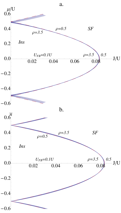
Figure 1: Zero-temperature mean-field phase diagram of the Fermi-Bose mixture with $U_{FB}=0.1U$. (a) Renormalized chemical potential, $\tilde{\mu}/U$ vs. bare $J/U$ phase boundary. From bottom-left to top-right, the fermions DOS is $\rho\cdot U=3.5,3,2.5,\ldots,0.5$. A dashed red line marks the uncoupled Bose gas, $U_{FB}=0$, but can barely be distinguished from the $\rho=0.5$ line. (b) charge-offset $\overline{n}=\tilde{\mu}/\tilde{U}$ vs. bare $J/U$ phase boundary. From left to right at $\overline{n}=0$, the fermions DOS is $\rho\cdot U=3.5,3,2.5,\ldots,0.5$.

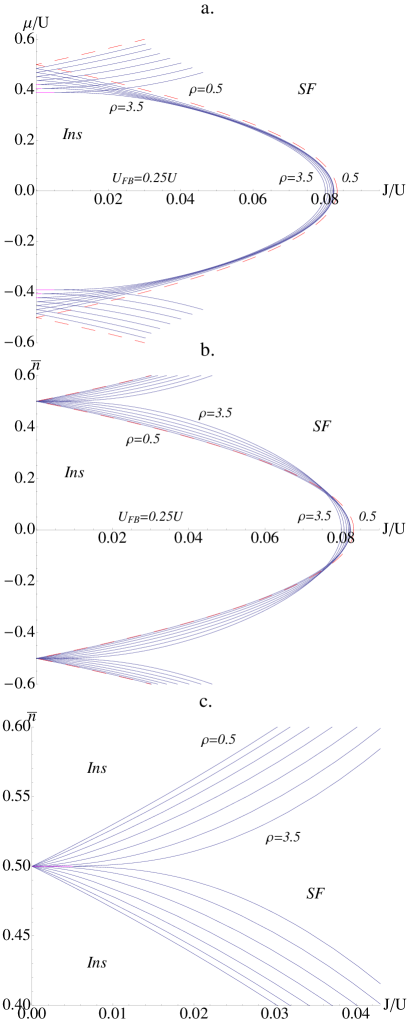
Figure 2: Zero-temperature mean-field phase diagram of the Fermi-Bose mixture with $U_{FB}=0.25U$. (a) Renormalized chemical potential, $\tilde{\mu}/U$ vs. bare $J/U$ phase boundary. From bottom-left to top-right, the fermions DOS is $\rho\cdot U=3.5,3,2.5,\ldots,0.5$. The dashed red line is the uncoupled Bose gas, $U_{FB}=0$. (b) charge-offset $\overline{n}=\tilde{\mu}/\tilde{U}$ vs. bare $J/U$ phase boundary. From left to right at $\overline{n}=0$, the fermions DOS is $\rho\cdot U=3.5,3,2.5,\ldots,0.5$. (c) A focus on the area near degeneracy, $\overline{n}=1/2$, in (b). In this plot we can see the strong effect of the orthogonality catastrophe for slow electrons. The intercept of the boundary with the $\overline{n}$ axis becomes singular and scales as $J/U\sim|0.5-\overline{n}|^{1-\gamma}$, illustrating Eq. (34).

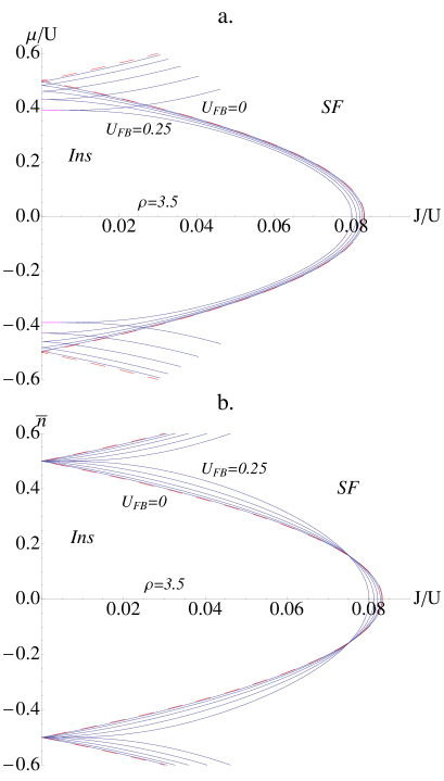
Figure 3: Zero-temperature mean-field phase diagram of the Fermi-Bose mixture with Fermi dispersion $\rho=3.5/U$. (a) Renormalized chemical potential, $\tilde{\mu}/U$ vs. bare $J/U$ phase boundary. From bottom-left to top-right, the fermions DOS is $U_{FB}/U=0,0.05,0.1,\ldots,0.25$. $U_{FB}=0$ is shown as a dashed red line. (b) Charge-offset $\overline{n}=\tilde{\mu}/\tilde{U}$ vs. bare $J/U$ phase boundary. From left to right at $\overline{n}=0$, the fermions DOS is $U_{FB}/U=0.25,0.2,\ldots,0$, with $U_{FB}=0$ shown as a red dashed line.

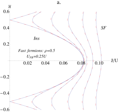
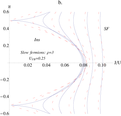
Figure 4: Temperature dependence of the SF-Ins boundary for $U_{FB}=0.25U$. (a) The SF-Ins boundary for $T=0,0.04,\ldots,0.2$ (from left to right at $\overline{n}=1/2$) with fast fermions, $\rho=0.5$. The dashed red line is the uncoupled Bose gas boundary, $U_{FB}=0$. (b) Same as (a) with slow Fermions, $\rho=3/U$. (c) The critical boson hopping $J/U$ vs. $T/U$, for fermion DOS $\rho\cdot U=0.5,1,\ldots,3.5$. The linear curve of the uncoupled Bose gas becomes a cusp as the bosons couple to slow fermions, as also calculated in Eq. (33).

Eq. (32) allows us to calculate the mean-field SF-insulator phase boundary for weakly interacting mixtures for a range of Temperatures and Fermi DOS. To illustrate Eq. (32) predictions for the transition line, Figs. 1, and 2 show the boundaries for Bosons and Fermions interacting with $U_{FB}=0.1U$ and $U_{FB}=0.25U$, respectively, for a range of fermion velocities, or DOS $\rho$. In Fig. 3 we plot the effect of slow fermions, with $\rho=3.5/U$, on the Bosonic SF transition for a range of interactions $U_{FB}$. The Superfluid-insulator transition boundary at finite temperature for $U_{FB}=0.25U$ is shown in Fig. 4 for a range of temperatures for fast and slow fermions. In all figures we assume $z=6$.

One easily drawn qualitative conclusion is that slow electrons mostly inhibit superfluidity, which is the mark of the orthogonality catastrophe. The most dramatic suppression effect occurs near the degeneracy points, where $\overline{n}=\tilde{\mu}/\tilde{U}=m+1/2$. Let us obtain closed-form expressions for the SF-INS boundary there. A helpful observation is that if the charging gap nearly vanishes, it suffices to consider the lowest nearly-degenerate charge states in Eq. (32).

When the degeneracy is exact, e.g., at $\overline{n}=1/2$, we obtain for the critical $J$ vs. Temperature:

$$\begin{array}[]{c}1=\frac{zJ}{4}\int\limits_{0}^{\beta}d\tau\left(\frac{\sin(\pi T/\Lambda)}{\sin(\pi T\tau)}\right)^{\gamma}\approx\\ \frac{zJ}{4\pi T}\left(\frac{2\pi T}{\Lambda}\right)^{\gamma}B(\frac{\gamma}{2},1-\gamma)\sin\left(\frac{\pi\gamma}{2}\right)\end{array}$$ (33)

where we neglected screening retardation, i.e., $S^{\Lambda}$, altogether. This is valid for $T^{1-\gamma}\ll\Lambda^{1-\gamma}/\gamma$. $B(m,n)$ is the beta-function. Fig. 4b shows Eq. (32) in this limit. Whereas for pure bosons the critical $J$ is linearly proportional to $T$, the interaction with Fermions makes the critical $J$ required for superfluidity increase dramatically, and obey $J_{c}\sim T^{1-\gamma}$.

A similar analysis can be done at zero temperature slightly away from degeneracy at $\overline{n}-1/2=\epsilon\ll 1$. In this regime we obtain:

$$1=\frac{zJ}{4}\int\limits_{0}^{\infty}d\tau\frac{e^{-\epsilon\tilde{U}\tau}}{\left(\Lambda\tau\right)^{\gamma}}\approx\\ \frac{zJ}{4}\left(\frac{\epsilon\tilde{U}}{\Lambda}\right)^{\gamma}\frac{1}{\epsilon\tilde{U}}\Gamma(1-\gamma).$$ (34)

where ignoring screening retardation is valid if $\epsilon^{1-\gamma}\ll(\Lambda/\tilde{U})^{1-\gamma}/\gamma$. Here too, the critical hopping as a function of $\epsilon$ is linear, $J_{c}\sim|\epsilon|$ for pure Bosons, but increases dramatically to $J_{c}\sim|\epsilon|^{1-\gamma}$ when the Bosons interact with the Fermions. This dependence is demonstrated in Fig. 2c.

V Discussion

V.1 Regime of applicability

Our theory of the SF-insulator transition applies to the weakly coupled Bose-Fermi mixtures, with $U_{FB}<U$, but a second parameter that is required to be small is $U_{FB}\rho<1$ (see Eq. 18). The latter is required for the perturbation theory of Eq. (23) to be justified. As explained above, this condition can be easily understood by noting from Eq. (15) that the response of the Fermi gas to the appearance of a Boson in a particular site is $\Delta n_{F}=U_{FB}\rho$, which clearly must be lower than 1. Even more importantly, the perturbative analysis is valid so long that no localized states form in the fermionic spectrum when a site’s potential changes by $U_{FB}$; this, too, is true when $\rho U_{FB}<1$ at large dimensionality.

The formation of a localized state at larger values of $U_{FB}\rho$, and therefore where $\gamma>1$, is likely to suppress the orthogonality-catastrophe effects, perhaps in analogy to the behavior of a Kondo-impurity in a metal: when a Kondo impurity localizes an electronic state it becomes inert. Therefore the largest suppression of the SF-INS boundary is likely to occur when $U_{FB}\rho\sim 1$, as $\gamma\sim 1$foo (a). The regime $\gamma>1$ lies beyond the scope of this paper, but we intend to approach it in a later publication. Note that this regime can still occur when $U_{FB}\ll U$.

We note also that since our theory is concerned with weak Fermi-Bose coupling, it ignores Fermi-Bose bound pair formation, as well as p-wave superconducting correlations, which may be important only at parametrically low temperatures.

V.2 Relation to experiment

Our theory provides the mean-field phase diagram under the assumption of a grand-canonical ensemble with fixed chemical potentials. Experiments, on the other hand, are conducted in finite non-uniform traps, and therefore to compare their results with the thermodynamic phase diagram we provide, the chemical potential of the interacting Bose and Fermi gasses must be determined for particular trap geometries, using, e.g., the LDA approach, as in Refs. Cramer et al., 2004; Albus et al., 2003.

Experiments on Bose-Fermi systems show a strong suppression of superfluidity. Ref. Gunter et al., 2006 describes a system where $J/U\sim 1/20$, $J_{F}/J\sim 5$, and $U_{FB}\sim-2U$, i.e., the Bose-Fermi system is strongly interacting. Thus our theory of orthogonality-catastrophe effects is not directly applicable here. We note, however, that at large values of $U_{FB}$, bound composite fermions would formLewenstein et al. (2004). These will have a weakened $U_{FB}$ and a strongly enhanced DOS, ${\rho}$. This makes it possible to observe orthogonality-catastrophe SF suppression even in this regime.

V.3 Relation to dissipative phase transitions

At weak $U_{FB}$, we find that Fermions, through their orthogonality catastrophe, by and large inhibit superfluidity, particularly when the fermions are slow. This effect is extremely reminiscent of dissipative superconducting-metal phase transitions in Josephson junctions.

Typically, dissipative effects as in resistively shunted Josephson junctions (RSJJ), are thought to strengthen phase coherence Schmid (1983); Chakravarty (1982). But in our case, since the Bose-Fermi mixtures couple through a capacitive interaction, as opposed to the phase-phase interaction in superconducting systems expressed in a Caldeira-Leggett Caldeira and Leggett (1981, 1983) term or its modular equivalent Ambegaokar et al. (1982), we encounter a suppression.

Another important distinction is that the Caldeira-Leggett analysis of a single RSJJ’s, and of 1d superfluids, associates (Quasi long-range) phase ordering with the long-time behavior of $\langle e^{i\phi(\tau)}e^{-i\phi(0)}\rangle$. But in the mean-field theory of the SF-insulator transition, the onset of true long-range phase order we encounter is associated with the less restrictive time-integral of the aforementioned correlation, as in Eq. (32) foo (b). The dynamics of the Fermionic screening gas modifies this integral only quantitatively, but it does not affect the nature of the transition.

The less restrictive condition for ordering in the mean-field analysis reflects the assumed higher dimensionality of the systems we consider. Concomitantly, in low dimensional systems with short-range interactions only, the Mermin-Wagner theorem rules out the formation of long range order. For Josephson junctions, for instance, phase-slips are the domain-wall like defects which make the order parameter fluctuate. Similar defects are absent from our analysis since their cost in terms of action is too prohibitive due to the assumed high connectivity of the system. Therefore we can make the mean-field assumption of a non-fluctuating order parameter. This assumption is fully justified above the lower critical dimension (although our analysis will only be valid at and above the upper critical dimension).

V.4 Summary and future directions

In this manuscript we concentrated on the effects of the orthogonality catastrophe on the superfluid-insulator transition line, and showed how slow fermions inhibit superfluidity through dissipation capacitatively coupled to number-fluctuations. The orthogonality catastrophe should also be evident in other measurements, which may give an independent estimate of the dissipation present. This might be most apparent in revival experiments, where the system is shifted from a superfluid phase into the insulating phase, and released after $t_{w}$ Greiner et al. (2002). We expect that the revival decay time will be smaller with increasing dissipation. We intend to address the dynamical effects in Fermi-Bose mixtures in a future work.

Another interesting angle for future work is the appearance of a super-solid at the special point of Fermionic half-filling Titvinidze et al. , extending our formalism to account for this possibility could be done by considering the Fermionic density correlations near nesting vectors of the Fermi gas.

Appendix A Fermionic response function

For completeness, we provide here a simple derivation of the Fermionic response function, Eq. (25), for fermions in one-dimension. Once our result is put in terms of the fermionic density-of-states at the Fermi-surface, it applies in any dimension, since the existence of a $(d-1)$-dimensional Fermi-surface renders the dispersion for low-energy excitations essentially one-dimensional.

Let us assume, for simplicity, that the fermionic Hamiltonian is:

$${\cal H}=\hbar v_{F}\sum\limits_{k=0}^{2k_{F}}(|k|-k_{F})(\hat{c}^{\dagger}_{k}\hat{c}_{k}+\hat{c}^{\dagger}_{-k}\hat{c}_{-k})$$ (35)

The density of states per site for this Hamiltonian is:

$$\rho=\frac{1}{\pi\hbar v_{F}}$$ (36)

For the Hamiltonian (35), Eq. (24) reads:

$$C_{\omega}=\langle\Delta n_{F\,i}\Delta n_{F\,i}(0)\rangle_{\omega}=T\frac{1}{V^{2}}\sum\limits_{k_{1},k_{2}=-2k_{F}}^{k_{F}}\sum\limits_{\omega^{\prime}=2\pi(n+1/2)}\frac{-1}{(i\omega^{\prime}-\hbar v_{F}(|k_{1}|-k_{F}))(i(\omega^{\prime}+\omega)-\hbar v_{F}(|k_{2}|-k_{F}))},$$ (37)

This formula sums over the contributions of particle-hole excitations of four kinds: both particle and hole are right movers ($k_{1},k_{2}>0$), both particle and hole are left movers ($k_{1},k_{2}<0$), and two mixed cases. In order to avoid the absolute value, we concentrate on the first case, and multiply by four:

$$C_{\omega}=4T\sum\limits_{\omega^{\prime}=2\pi(n+1/2)+\omega/2}\int_{0}^{2k_{F}}\frac{dk_{1}}{2\pi}\int_{0}^{2k_{F}}\frac{dk_{2}}{2\pi}\frac{1}{i(\omega^{\prime}-\omega/2)-\hbar v_{F}(k_{1}-k_{F})}\frac{1}{i(\omega^{\prime}+\omega/2)-\hbar v_{F}(k_{2}-k_{F})},$$ (38)

where we also shifted $\omega^{\prime}$ by $\omega/2$. We now separate from this sum the contributions from large $|\omega^{\prime}|>\hbar v_{F}k_{F}$. These high energy modes contribute an $\omega$-independent term to the static screening. Corrections to this constant are easily seen to be quadratic in $\omega$ (e.g., set $k_{1},k_{2}\rightarrow 0$). The low-$\omega^{\prime}$ terms, however, will give rise to a $|\omega|$ contribution, which we are after. The k-integrals can be easily done in the limit $|\omega^{\prime}\pm\omega/2|\ll\hbar v_{F}k_{F}$, and we obtain:

$$\begin{array}[]{c}C_{\omega}=c-4T\sum\limits_{\omega^{\prime}=2\pi(n+1/2)+\omega/2}\frac{1}{(2\pi\hbar v_{F})^{2}}\log\left(\frac{\hbar v_{F}k_{F}-i(\omega^{\prime}-\omega/2)}{-\hbar v_{F}k_{F}-i(\omega^{\prime}-\omega/2)}\right)\log\left(\frac{\hbar v_{F}k_{F}-i(\omega^{\prime}+\omega/2)}{-\hbar v_{F}k_{F}-i(\omega^{\prime}+\omega/2)}\right)\vspace{2mm}\\ \approx c-4T\sum\limits_{\omega^{\prime}=2\pi(n+1/2)+\omega/2}\frac{1}{(2\pi\hbar v_{F})^{2}}[-i\pi~{}\rm{sgn}(\omega^{\prime}+\omega/2)][-i\pi~{}\rm{sgn}(\omega^{\prime}-\omega/2)].\end{array}$$ (39)

The $\omega$ dependence arises from the region where the two sign functions give opposite results: $-|\omega|/2<\omega^{\prime}<|\omega|/2$. Thus:

$$C_{\omega}=c^{\prime}-4T\frac{|\omega|}{2\pi T}\frac{1}{(2\hbar v_{F})^{2}}\cdot 2,$$ (40)

where the last factor of 2 is since $c^{\prime}$ contains the contributions for $-|\omega|/2<\omega^{\prime}<|\omega|/2$ assuming the same sign as for the rest of the frequency range. The final answer is thus:

$$C_{\omega}=c^{\prime}-\frac{|\omega|}{\pi v_{F}^{2}\hbar^{2}}=a-\pi\rho^{2}|\omega|,$$ (41)

as reported in Eq. (25).

A.1 Bosonization approach to the polarization calculation

One-dimensional fermionic systems are most effectively described in terms of a bosonized action. Let us re-derive Eq. (25) using this simpler approach. We define the two fields $\theta$ and $\phi$. Using here the convention:

$$\frac{1}{\pi}\nabla\theta=\rho_{L}+\rho_{R}\hskip 14.22636pt\frac{1}{\pi}\nabla\phi=\rho_{R}-\rho_{L},$$ (42)

where $\rho_{R,L}$ are the right-moving and left-moving densities respectively, the Hamiltonian of 1-d Fermions is:

$${\cal H}=\frac{v_{F}\hbar}{2\pi}\int dx\left(\nabla\theta^{2}+\nabla\phi^{2}\right),$$ (43)

and $v_{F}$ is the Fermi velocity.

The Hamiltonian (43) can be turned into an imaginary time Lagrangian:

$${\cal L}=\frac{v_{F}\hbar}{2\pi}\int dx\left(\nabla\theta^{2}+\dot{\theta}^{2}\right).$$ (44)

The density-density correlation we would like to calculate is now given as a path-integral over the $\theta$ field:

$$C_{\omega}=\langle\Delta n_{F\,i}\Delta n_{F\,i}(0)\rangle_{\omega}=2\cdot\frac{1}{\pi^{2}}\langle\nabla\theta\nabla\theta\rangle_{\omega}$$ (45)

Here we need to pause and explain the extra factor of 2: the expectation value in the brackets only takes into account particle-hole excitations that are contained within the same branch of the fermionic spectrum, right moving or left moving. We must also include, however, excitations with the particle part being a right mover and the hole being a left mover, and vise versa. These give exactly the same contribution (as is also seen in the first approach), and therefore it is sufficient to simply multiply the expectation value by 2.

With that in mind, we proceed to write:

$$\begin{array}[]{c}C_{\omega}=\frac{2}{\pi^{2}}\int\limits_{-k_{F}}^{k_{F}}\frac{dk}{2\pi}\frac{k^{2}}{\frac{2v_{F}\hbar}{2\pi}\left(k^{2}+\omega^{2}/v_{F}^{2}\right)}\vspace{2mm}\\ \frac{1}{\pi^{2}v_{F}\hbar}\int\limits_{-k_{F}}^{k_{F}}dk\left[1-\frac{\omega^{2}/v_{F}^{2}}{k^{2}+\omega^{2}/v_{F}^{2}}\right]\vspace{2mm}\\ \approx c^{\prime}-\frac{\omega^{2}}{\pi^{2}v_{F}^{3}\hbar}\int\limits_{\infty}^{\infty}\frac{dk}{k^{2}+(\omega/v_{F})^{2}}\vspace{2mm}\\ =c^{\prime}-|\omega|\frac{1}{\pi v_{F}^{2}\hbar^{2}}=c^{\prime}-\pi\rho^{2}|\omega|,\end{array}$$ (46)

where in the last step we simply calculated the residue of the k integral.

References

- Haviland et al. (1989) D. B. Haviland, Y. Liu, and A. M. Goldman, Phys. Rev. Lett. 62, 2180 (1989).
- Hebard and Paalanen (1990) A. F. Hebard and M. A. Paalanen, Phys. Rev. Lett. 65, 927 (1990).
- Steiner et al. (2005) M. A. Steiner, G. Boebinger, and A. Kapitulnik, Phys. Rev. Lett. 94, 107008 (2005).
- Sambandamurthy et al. (2004) G. Sambandamurthy, L. W. Engel, A. Johansson, and D. Shahar, Phys. Rev. Lett. 92, 107005 (2004).
- Frydman et al. (2002) A. Frydman, O. Naaman, and R. C. Dynes, Phys. Rev. B 66, 052509 (2002).
- Lau et al. (2001) C. N. Lau, N. Markovic, M. Bockrath, A. Bezryadin, and M. Tinkham, Phys. Rev. Lett. 87, 217003 (2001).
- Bezryadin et al. (2000) A. Bezryadin, C. N. Lau, and M. Tinkham, Nature 404, 971 (2000).
- Rogachev and Bezryadin (2003) A. Rogachev and A. Bezryadin, Applied Physics Letters 83, 512 (2003).
- Altomare et al. (2006) F. Altomare, A. M. Chang, M. R. Melloch, Y. Hong, and C. W. Tu, Phys. Rev. Lett. 97, 017001 (2006).
- Haviland et al. (2000) D. B. Haviland, K. Andersson, and P. Ågren, J. of Low T. Phys. 118, 733 (2000).
- Chow et al. (1998) E. Chow, P. Delsing, and D. B. Haviland, Phys. Rev. Lett. 81, 204 (1998).
- Rimberg et al. (1997) A. J. Rimberg, T. R. Ho, C. Kurdak, J. Clarke, K. L. Campman, and A. C. Gossard, Phys. Rev. Lett. 78, 2632 (1997).
- Zhang et al. (1989) S. C. Zhang, T. H. Hansson, and S. Kivelson, Phys. Rev. Lett. 62, 82 (1989).
- Oshikawa et al. (1997) M. Oshikawa, M. Yamanaka, and I. Affleck, Phys. Rev. Lett. 78, 1984 (1997).
- Fisher (1990) M. P. A. Fisher, Phys. Rev. Lett. 65, 923 (1990).
- Sachdev (1999) S. Sachdev, Quantum phase transitions (Cambridge University Press, London, 1999).
- Fisher et al. (1989) M. P. A. Fisher, P. B. Weichman, G. Grinstein, and D. S. Fisher, Phys. Rev. B 40, 546 (1989).
- Mason and Kapitulnik (2002) N. Mason and A. Kapitulnik, Phys. Rev. B 65, 220505 (2002).
- Mason and Kapitulnik (1999) N. Mason and A. Kapitulnik, Phys. Rev. Lett. 82, 5341 (1999).
- Refael et al. (2007) G. Refael, E. Demler, Y. Oreg, and D. S. Fisher, Phys. Rev. B 75, 014522 (2007).
- Michaeli and Finkel’stein (2006) K. Michaeli and A. M. Finkel’stein, Phys. Rev. Lett. 97, 117004 (2006).
- Vishwanath et al. (2004) A. Vishwanath, J. E. Moore, and T. Senthil, Phys. Rev. B 69, 054507 (2004).
- Bloch et al. (2007) I. Bloch, J. Dalibard, and W. Zwerger, Many-body physics with ultracold gases, arXiv.org:0704.3011 (2007).
- Cramer et al. (2004) M. Cramer, J. Eisert, and F. Illuminati, Phys. Rev. Lett. 93, 190405 (2004).
- Albus et al. (2003) A. Albus, F. Illuminati, and J. Eisert, Phys. Rev. A 68, 023606 (2003).
- Wang (2006) D.-W. Wang, Phys. Rev. Lett. 96, 140404 (2006).
- (27) I. Titvinidze, M. Snoek, and W. Hofstetter, cond-mat/0708.3241.
- Büchler and Blatter (2004) H. P. Büchler and G. Blatter, Phys. Rev. A 69, 063603 (2004).
- Adhikari and Salasnich (2007) S. K. Adhikari and L. Salasnich, Phys. Rev. A 76, 023612 (2007).
- Lewenstein et al. (2004) M. Lewenstein, L. Santos, M. A. Baranov, and H. Fehrmann, Phys. Rev. Lett. 92, 050401 (2004).
- Powell et al. (2005) S. Powell, S. Sachdev, and H. P. Buchler, Phys. Rev. B 72, 024534 (2005).
- Gunter et al. (2006) K. Gunter, T. Stoferle, H. Moritz, M. Kohl, and T. Esslinger, Phys. Rev. Lett. 96, 180402 (2006).
- Ospelkaus et al. (2006a) C. Ospelkaus, S. Ospelkaus, K. Sengstock, and K. Bongs, Phys. Rev. Lett. 96, 020401 (2006a).
- Schreck et al. (2001) F. Schreck, L. Khaykovich, K. L. Corwin, G. Ferrari, T. Bourdel, J. Cubizolles, and C. Salomon, Phys. Rev. Lett. 87, 080403 (2001).
- Ospelkaus et al. (2006b) S. Ospelkaus, C. Ospelkaus, O. Wille, M. Succo, P. Ernst, K. Sengstock, and K. Bongs, Phys. Rev. Lett. 96, 180403 (2006b).
- Modugno et al. (2003) M. Modugno, F. Ferlaino, F. Riboli, G. Roati, G. Modugno, and M. Inguscio, Phys. Rev. A 68, 043626 (2003).
- Ferlaino et al. (2004) F. Ferlaino, E. de Mirandes, G. Roati, G. Modugno, and M. Inguscio, Phys. Rev. Lett. 92, 140405 (2004).
- Hadzibabic et al. (2002) Z. Hadzibabic, C. A. Stan, K. Dieckmann, S. Gupta, M. W. Zwierlein, A. Görlitz, and W. Ketterle, Phys. Rev. Lett. 88, 160401 (2002).
- (39) S. Roethel and A. Pelster, cond-mat/0703220.
- (40) L. Pollet, C. Kollath, U. Schollwöck, and M. Troyer, cond-mat/0609604.
- Wen (2004) X.-G. Wen, Quantum Field Theory of Many-body Systems (Oxford University Press, 2004).
- Mahan (1981) G. D. Mahan, Many-Particle Physics (AP, 1981).
- Anderson (1967) P. W. Anderson, Phys. Rev. Lett. 18, 1049 (1967).
- Yang (2007) K. Yang, Superfluid-insulator transition and fermion pairing in bose-fermi mixtures, arXiv.org:0707.4189 (2007).
- Mering and Fleischhauer (2007) A. Mering and M. Fleischhauer, The one-dimensional bose-fermi-hubbard model in the heavy-fermion limit, arXiv.org:0709.2386 (2007).
- Mathey et al. (2004) L. Mathey, D.-W. Wang, W. Hofstetter, M. D. Lukin, and E. Demler, Phys. Rev. Lett. 93, 120404 (pages 4) (2004).
- Sengupta and Pryadko (2005) P. Sengupta and L. P. Pryadko, Quantum degenerate bose-fermi mixtures on 1-d optical lattices, cond-mat/0512241 (2005).
- Altman and Auerbach (1998) E. Altman and A. Auerbach, Phys. Rev. Lett. 81, 4484 (1998).
- Noziéres and De Dominicis (1969) P. Noziéres and C. T. De Dominicis, Phys. Rev. 178, 1097 (1969).
- Yuval and Anderson (1970) G. Yuval and P. W. Anderson, Phys. Rev. B 1, 1522 (1970).
- Caldeira and Leggett (1981) A. O. Caldeira and A. J. Leggett, Phys. Rev. Lett. 46, 211 (1981).
- Caldeira and Leggett (1983) A. O. Caldeira and A. J. Leggett, Ann. Phys. 149, 374 (1983).
- foo (a) But since can not exceed 1, the qualitative nature of the SF-INS transition is always the same, and never becomes a Caldeira-Leggett type transition.
- Schmid (1983) A. Schmid, Phys. Rev. Lett. 51, 1506 (1983).
- Chakravarty (1982) S. Chakravarty, Phys. Rev. Lett. 49, 681 (1982).
- Ambegaokar et al. (1982) V. Ambegaokar, U. Eckern, and G. Schön, Phys. Rev. Lett. 48, 1745 (1982).
- foo (b) Note, also, that the mean-field is strictly only valid at , and long-range phase ordering may only appear at by the Mermin-Wagner theorem.
- Greiner et al. (2002) M. Greiner, O. Mandel, T. W. Hänsch, and I. Bloch, Nature 419, 51 (2002).