Landau-deGennes Theory of Biaxial Nematics Re-examined

Abstract

Recent experiments report that the long looked for thermotropic biaxial nematic phase has been finally detected in some thermotropic liquid crystalline systems. Inspired by these experimental observations we concentrate on some elementary theoretical issues concerned with the classical sixth-order Landau-deGennes free energy expansion in terms of the symmetric and traceless tensor order parameter $Q_{\alpha\beta}$. In particular, we fully explore the stability of the biaxial nematic phase giving analytical solutions for all distinct classes of the phase diagrams that theory allows. This includes diagrams with triple- and (tri-)critical points and with multiple (reentrant) biaxial- and uniaxial phase transitions. A brief comparison with predictions of existing molecular theories is also given.

I INTRODUCTION

The biaxial nematic phase, predicted theoretically by Freiser Freiser (1970, 1971) over 35 years ago, is one of the perennially challenging problems of experimental soft-matter physics. Although discovery of this phase was made by Saupe and co-workers in a fine-tuned lyotropic liquid crystal system in 1980 Yu and Saupe (1980) only in the past three years- and following several earlier attempts that proved unsuccessful in this regard (for a comprehensive review see e.g. Luckhurst (2001, 2004))- strong experimental evidence has become available that this phase can also be made stable in thermotropic liquid crystalline materials Madsen et al. (2004); Acharya et al. (2004); Merkel et al. (2004); Madsen et al. (2006). This discovery raises the emerging theoretical problem of what mechanism is responsible for the stability of thermotropic biaxial nematics, especially for bent-core systems Madsen et al. (2004); Acharya et al. (2004) and for tetrapode-like molecules Merkel et al. (2004); Neupane et al. (2006), where this phase was shown to be stable.

There are two nematic phases of distinct symmetries. The ubiquitous uniaxial nematic phase has the ${\cal{D}}_{\infty h}$ point group symmetry de Gennes and Prost (1993); Gramsbergen et al. (1986); Singh (2000); Longa et al. (1994), which results in the definition of a single mesoscopic direction, known as the director. The director is a unit vector, denoted $\mathbf{\hat{n}}$, with the directions $\mathbf{\bf\hat{n}}$ and $-\mathbf{\hat{n}}$ being equivalent. One consequence of this is that there are two different principal components of a second rank tensorial property, such as e.g the magnetic susceptibility. Generally, two uniaxial nematic phases are distinguished: prolate ($N_{U+}$) and oblate ($N_{U-}$). The prolate uniaxial states usually occur for rod-like molecules while disc-like molecules yield the oblate uniaxial states. As opposed to the uniaxial nematic phase, the biaxial nematic phase, denoted $~{}N_{B}$, is characterized by three orthonormal directors, the Goldstone modes, which we denote $\{\mathbf{\hat{l}},\mathbf{\hat{m}},\mathbf{\hat{n}}=\mathbf{\hat{l}}\times\mathbf{\hat{m}}\}$. Due to overall lack of polarity of the known biaxial nematics, one finds that $\mathbf{\hat{l}}$ and $-\mathbf{\hat{l}}$, $\mathbf{\hat{m}}$ and $-\mathbf{\hat{m}}$ and $\mathbf{\hat{n}}$ and $-\mathbf{\hat{n}}$ directions are equivalent. That is, from the symmetry point of view the biaxial nematic phase is a structure of ${\cal{D}}_{2h}$ point-group symmetry and the corresponding second rank tensorial property has three different principal components.

Generally, first– and second order phase transitions are observed experimentally between the isotropic phase and different nematic phases and between the nematic phases. The phase sequence of $Iso$ $\leftrightarrow$ $(N_{U-})$ $\leftrightarrow$ $(N_{B})$ $\leftrightarrow$ $(N_{U+})$ $\leftrightarrow$ $(N_{B})$ $\leftrightarrow$ $(N_{U-})$ $\leftrightarrow$ $(Iso)$ is found with decreasing temperature Yu and Saupe (1980); Charvolin (1984); Neto and Salinas (2005); Merkel et al. (2004), where the brackets indicate that some of the phases may not appear. In particular, the amazing reentrant uniaxial and isotropic phases are observed in lyotropic systems (see e.g. Neto and Salinas (2005) and references therein).

On the theoretical level, possible effects of molecular structure on nematic order have been studied. More specifically, molecular field theories of single-component systems consisting of biaxial molecules and interacting via hard-core or continuous potentials were shown to produce a stable biaxial phase Freiser (1970); Alben (1973); Mulder (1989); Teixeira et al. (1998); Sonnet et al. (2003); Longa et al. (2005, 2007). A similar scenario emerges from computer simulation studies Biscarini et al. (1995); Cleaver et al. (1996); Sarman (1996); Camp and Allen (1997); Ginzburg et al. (1997); Camp et al. (1999); Berardi and Zannoni (2000) and from Landau treatments Allender and Lee (1984); Allender et al. (1985); Gramsbergen et al. (1986); Prostakov et al. (2002).

Out of the theories cited the simplest description of the uniaxial and biaxial nematic phases is one offered by a sixth-order Landau-deGennes free energy expansion in terms of the alignment tensor $Q_{\alpha\beta}$ (6). The theory is generally employed to interpret experimental data as well as to classify possible topologies of the phase diagrams. Therefore it seems quite important to know, if possible, an analytical form of all distinct classes of the phase diagrams and limitations on them that can be derived from this simple theory. This task has only partly been realized so far Allender and Lee (1984); Allender et al. (1985); Gramsbergen et al. (1986); Toledano et al. (1995); Longa et al. (1998); Singh (2000); Prostakov et al. (2002). None of the papers cited shows, however, a full spectrum of predictions of this theory. The closest to the ideal is the paper by Prostakov Prostakov et al. (2002), but also there not all cases/analytical solutions have been given.

Owing to the current excitement in the field of thermotropic biaxial nematics we think it is important to re-examine this fundamental theory. We give analytical formulas for all distinct classes of the phase diagrams the model can predict and for their stability range. We hope this will be of some help for experimentalists in analyzing experimental data on biaxial nematics and will bring partial order to existing molecular predictions on this phase.

This paper is organized as follows. After a brief discussion of the Landau-deGennes theory in Sec. II, we give analytical solutions for the phase diagrams in Sec. III. Section IV is devoted to a short discussion.

II Landau-deGennes Free Energy

The best way to account for a symmetry change that takes place across a phase transition is by referring to an order parameter. For a phenomenological description of the nematics the relevant order parameters are tensors built out of the directors. Among these the leading order parameter is the second rank symmetric and traceless alignment tensor $\mathbf{Q}$. In a standard parametrization $\mathbf{Q}$ can be written as

$$\mathbf{Q} = {\frac{q_{0}}{\sqrt{6}}}\left(3\hat{\mathbf{n}}\otimes\hat{\mathbf{n}}-{\bm{1}}\right)+{\frac{q_{2}}{\sqrt{2}}}\left(\hat{\mathbf{l}}\otimes\hat{\mathbf{l}}-\hat{\mathbf{m}}\otimes\hat{\mathbf{m}}\right),$$ (1)

where the directors {$\mathbf{\hat{l}},\mathbf{\hat{m}},\mathbf{\hat{n}}$} are identified with eigenvectors of $\mathbf{Q}$ corresponding to the eigenvalues $\lambda_{1}=-\frac{{q_{0}}}{\sqrt{6}}+\frac{{q_{2}}}{\sqrt{2}}$, $\lambda_{2}=-\frac{q_{0}}{\sqrt{6}}-\frac{q_{2}}{\sqrt{2}}$, $\lambda_{3}=-\lambda_{1}-\lambda_{2}=\sqrt{\frac{2}{3}}q_{0}$, respectively. The parametrization (1) for $\mathbf{Q}$ is chosen such that the formula for $F$ is kept concise. The isotropic state is stabilized when all three eigenvalues of ${\mathbf{Q}}$ are equal and hence vanish, which yields ${\mathbf{Q}}\equiv{\mathbf{0}}$. For the ${\cal{D}}_{\infty h}$- symmetric uniaxial states two out of the three eigenvalues of ${\mathbf{Q}}$ are equal, i.e., $q_{0}\neq 0,\,q_{2}=0$ or $q_{0}\neq 0,\,q_{2}=\sqrt{3}\,q_{0}$ or $q_{0}\neq 0,\,q_{2}=-\sqrt{3}\,q_{0}$. In the general case, ${\mathbf{Q}}$ has three different real eigenvalues that account for the ${\cal{D}}_{2h}$- symmetric biaxial state. A microscopic interpretation of the alignment tensor for simple molecular models is found in Mulder (1989); Longa and Paja̧k (2005) and can easily be extended to the more general cases.

The Landau-deGennes phenomenological theory of non-chiral systems is implicitly based on the hypothesis that equilibrium properties of the system can be found from a non-equilibrium free energy, constructed as an ${\cal{O}}(3)$–symmetric expansion in powers of $\mathbf{~{}Q}$. The only restriction on the expansion is that it must be stable against an unlimited growth of the order parameter. There are two types of ${\cal{O}}(3)$ invariants that can be constructed out of $\mathbf{Q}$, which involve traces and determinants of powers of $\mathbf{Q}$. But determinants can be expressed in terms of traces and all traces of $\mathbf{Q}^{n}$ with $n\geq 4$ are polynomials of $\mathrm{Tr}{(\mathbf{Q}}^{2})$ and $\mathrm{Tr}{(\mathbf{Q}}^{3})$ Gramsbergen et al. (1986). In addition, $\mathrm{Tr}{(\mathbf{Q}}^{2})$ and $\mathrm{Tr}{(\mathbf{Q}}^{3})$ are bounded by the inequality

$$\frac{1}{6}\mathrm{Tr}{(\mathbf{Q}}^{2})^{3}-\mathrm{Tr}{(\mathbf{Q}}^{3})^{2}=\hskip 113.81102pt$$

$$\frac{1}{3}\left(\lambda_{1}-\lambda_{2}\right)^{2}\left(2\lambda_{1}+\lambda_{2}\right)^{2}\left(\lambda_{1}+2\lambda_{2}\right)^{2}\geq 0,$$ (2)

which is fulfilled as equality for the uniaxial phases.

A coordinate-independent form of the inequality (II) is obtained by a very convenient re-parametrization in $\mathrm{Tr}(\mathbf{Q}^{2})$ and $\mathrm{Tr}(\mathbf{Q}^{3})$ that uses just two scalar parameters: $q$ and $0\leq\omega\leq 1$. They are introduced through the relations

$$\mathrm{Tr}(\mathbf{Q}^{2}) = q^{2}=q_{0}^{2}+q_{2}^{2}=I_{2}$$ (3)

$${\sqrt{6}}\,\mathrm{Tr}(\mathbf{Q}^{3}) = {q^{3}(1-\omega)}=q_{0}^{3}-3q_{0}q_{2}^{2}=I_{3},$$ (4)

where $|q|$ is the norm of $\mathbf{Q}$ and $\omega$ serves as a normalized measure of phase biaxiality. The ${\cal{D}}_{2h}$- symmetric biaxial state is characterized by $\omega>0$ with maximal biaxiality being accomplished for $\omega=1$. For the uniaxial phases $\omega=0$. In addition, for uniaxial $\mathbf{Q}$-tensors a transformation $\mathbf{\hat{u}}\rightarrow[(Q_{\alpha\beta}-c\delta_{\alpha\beta})u_{\alpha}u_{\beta}]$, where c is an arbitrary constant making the bilinear form $[...]$ positive-definite, transforms a unit sphere $|\mathbf{\hat{u}}|=1$ into an axially symmetric, prolate- ($q>0$) or oblate ($q<0$) closed surface. Hence the sign of $q$, being consistent with the sign of $\mathrm{Tr}(\mathbf{Q}^{3})$, allows one to distinguish between ${N_{U+}}$ ($q>0$) and ${N_{U-}}$ ($q<0$) phases. Actually $q$ and $\omega$ can serve as invariant measures of order in uniaxial ($q\neq 0,\omega=0$)- and biaxial ($q\neq 0,\omega\neq 0$) nematics. For the isotropic phase $q=0$. The allowed variation of $\mathrm{Tr}(\mathbf{Q}^{2})$ and $\mathrm{Tr}(\mathbf{Q}^{3})$ and consequently also of $q$ and $\omega$, along with the identification of different nematic phases, is shown in Fig. (1).

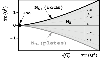
Figure 1: Allowed variation of the independent degrees of freedom $\mathrm{Tr}{(\mathbf{Q}}^{2})$ and $\mathrm{Tr}{(\mathbf{Q}}^{3})$ (shaded area) and identification of the corresponding phases. Shown are also lines of constant biaxiality parameter, $\omega$.

In the absence of electric and magnetic fields the bulk free energy for the isotropic- and the nematic phases has the form

$$F(\mathbf{Q})=F[\mathrm{Tr}{(\mathbf{Q}}^{2}),\mathrm{Tr}{(\mathbf{Q}}^{3})]=F[I_{2},I_{3}]=F[q,\omega].$$ (5)

The minimal coupling Landau expansion of $F$ that accounts for the biaxial nematic phase has to be taken up to 6th order with respect to $\mathbf{Q}$. This theory, also known as Landau-deGennes free energy of biaxial nematics, reads (see e.g. Gramsbergen et al. (1986))

$$F = F_{o}+\frac{1}{2}a\,I_{2}-\frac{1}{3}b\,I_{3}+\frac{1}{4}c\,I_{2}^{2}+\frac{1}{5}d\,I_{2}I_{3}+$$ (6)

$$\frac{1}{6}e\,I_{2}^{3}+\frac{1}{6}(f-e)I_{3}^{2}+\ldots$$

$$= F_{o}+F_{u}(q)+F_{b}(q)\omega+\frac{1}{6}\,\phi\,q^{6}\omega^{2}\ldots$$

with

$$F_{u} = \frac{1}{2}a\,q^{2}-\frac{1}{3}b\,q^{3}+\frac{1}{4}c\,q^{4}+\frac{1}{5}d\,q^{5}+\frac{1}{6}f\,q^{6}\hskip 28.45274pt$$ (7)

$$F_{b} = \frac{1}{3}b\,q^{3}-\frac{1}{5}d\,q^{5}-\frac{1}{3}\,\phi\,q^{6}.$$ (8)

In Eq. (6) the $F_{o}$-part represents the unimportant free energy of the reference isotropic phase; $F_{u}$ is the free energy of the uniaxial phases ($\omega=0$) and the remaining two terms represent biaxial contributions. The coefficients of the expansion generally depend on temperature (inverse density) and other thermodynamic (control) parameters. In what follows we will only keep an explicit dependence on the temperature. In particular, the coefficient $a=a_{o}(T-T^{*})$ with $T$ being the absolute temperature, is the only term in the expansion that is assumed to be explicitly temperature (or density)-dependent. On general thermodynamic grounds (see e.g. Longa and Paja̧k (2005)) one can show that $a$ is usually the first of the coefficients in the expansion (6) that changes sign as temperature is lowered. The sign change is a result of competition between either energy and entropy or different forms of entropy. The parameter $T^{*}$ accounts quantitatively for this competition and represents the spinodal temperature for the first order phase transition from the isotropic phase to the uniaxial nematic phase. As for the remaining parameters: $a_{o}>0$ by definition and stability of the expansion requires $e>0$ and $f>0$. Except for cases of multicritical behavior, the signs of $b,c,d,e,f$ are assumed not to change in the vicinity of $T^{*}$. Hence, these coefficients, being weakly temperature-dependent, are assumed constants and taken at $T=T^{*}$.

The parametrization of $F$ in terms of $q$ and $\omega$, Eq. (6), leads to a simple determination of absolute minima of $F$ and, hence, a construction of the corresponding phase diagrams. Clearly, the form of $\mathbf{Q}$, Eq. (1), implies that the Iso-$N_{B}$ and the $N_{U}-N_{B}$ phase transitions can be either first- or second order. In other words we may expect first-order, second-order and tricritical behavior at Iso-$N_{B}$ and $N_{U}-N_{B}$ transitions, depending on model parameters.

III Phase diagrams

Out of the five material parameters $b,c,d,e,f$ ($\phi=f-e$), introduced in Eq. (6), two are redundant and can be set equal to 0 or $\pm 1$. This is a direct consequence of the freedom to choose a scale for the free energy and for ${\mathbf{Q}}$. If not specified otherwise we choose $e=1$ and $c=0,\pm 1$, and investigate the phase diagrams in the ($a$, $b$)-plane as function of $d$ and $f$. Additionally, we assume $f>0$ to guarantee the stability of the expansion (6) against unlimited growth of $q$ and replace $f-e$ by $\phi$ ($\phi=f-e\equiv f-1$) whenever convenient. We also make use of the free energy invariance with respect to the transformation: $\{b,d,q\}\rightarrow\{-b,-d,-q\}$, which limits $d$ to $d\geq 0$. The diagrams for $d<0$ are obtained as mirror images with respect to the $b=0$ line of those for $d>0$, followed by a subsequent change of $N_{U\pm}$ into $N_{U\mp}$.

Interestingly, the relatively simple expansion (6) generates a rich spectrum of possibilities for phase diagrams. We show that all of them can be divided into ten distinct classes, where four involve only uniaxial phases. The remaining cases, corresponding to $d<0$, are obtained from the classes discussed by applying the aforementioned $b=0$ mirror transformation.

III.1 Phase diagrams with uniaxial phases: $q\neq 0,\omega=0$

We start by considering regions of stability of the uniaxial nematic. The necessary conditions for this phase to become, at least, locally stable read

$$\frac{\partial F_{u}}{\partial q} = q\left(a-bq+cq^{2}+dq^{3}+fq^{4}\right)=0$$ (9)

$$\frac{\partial^{2}F_{u}}{\partial q^{2}} = a-2bq+3cq^{2}+4dq^{3}+5fq^{4}>0.$$ (10)

The limit of local stability is attained when the inequality (10) becomes equality, which, together with (9), describes a saddle bifurcation in the model and represents spinodal lines. These conditions are particularly simple to solve for $a$ and $b$ in a parametric, q-dependent form. The nontrivial solution is

$$a = cq^{2}+2dq^{3}+3fq^{4}$$ (11)

$$b = 2cq+3dq^{2}+4fq^{3},$$ (12)

which, together with the trivial one: $\left\{a=0,q=0,(\forall\,b)\right\}$ defines the borders of the area in the $(a,b)$ plane, where the solutions to the Eq. (9) are, at least, locally stable. Clearly, $q$ runs over all real numbers. The subsequent calculation of the free energy at these local minima allows us to select the global minimum within the family of uniaxial solutions.

A complete analysis of the model, including calculation of the free energy, proceeds in a similar way. In particular, we determine parametrically the transition line between the isotropic- and the uniaxial phases by solving the system of equations: $\{F_{u}=0,\partial F_{u}/\partial q=0\}$ for $a(q)$ and $b(q)$. The solution reads

$$a = \frac{cq^{2}}{2}+\frac{4dq^{3}}{5}+fq^{4}$$ (13)

$$b = \frac{3cq}{2}+\frac{9dq^{2}}{5}+2fq^{3}.$$ (14)

Subsequent analysis of the Eqs. (11, 13) allows us to single out four topologically distinct classes of the phase diagrams with uniaxial- and isotropic phases. The representatives of each class are shown in Figs. 2-5. The corresponding global stability sectors in the $\{c,d,f\}$ parameter space are given in Figs.14-12.

We shall now characterize each of the ’uniaxial’ classes of the diagrams.

III.1.1 Class (a)

The first class is obtained for $d=0$, Fig. 2.

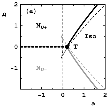
Figure 2: Generic phase diagram with a direct, first order phase transition from isotropic- to uniaxial nematic phases, where gray color refers to phase transitions involving the $N_{U-}$ phase. For $b=0$ a phase transition between isotropic and highly degenerated phase of $q\neq 0$ but of arbitrary $\omega$ takes place at the quadruple point (T). For $c>0$ T became a tetracritical point. Parameters taken are $(c,d,f)=(-1,0,1)$. Thin dashed lines, representing spinodal, are the solutions of the Eq. (11); also $a=0$ spinodal is shown.

It contains a line of first order $Iso\leftrightarrow{N_{U+}}$ phase transitions for $b>0$, a line of first order $Iso\leftrightarrow{N_{U-}}$ phase transitions for $b<0$, and a degenerated biaxial phase of $q\neq 0$ and arbitrary $\omega$, stable only along the $b=0$ line. We shall come back to the degenerated case in the last subsection of this paper. The $Iso\leftrightarrow{N_{U\pm}}$ lines have a common tangent $a=0$. For $c\geq 0$ the four lines meet at an isolated, tetracritical point, also often referred to as the Landau point. Its coordinates are $(a,b)=(0,0)$. For $c<0$ the Landau point becomes a quadruple point of coordinates $(a,b)=(\frac{3c^{2}}{16f},0)$, marked as ’T’ in Fig. 2. The whole phase diagram is given analytically by

$$b^{2}=\frac{\sqrt{\left(c^{2}+16af\right)^{3}}-c\left(c^{2}-48af\right)}{16f},$$ (15)

where $a\geq\frac{3c^{2}}{16f}\Theta(c)$ with $\Theta$ being the step function.

Now we concentrate on more complex cases with $d\neq 0$. They are gathered in three classes of the diagrams, denoted (b)-(d).

III.1.2 Class (b)

Diagrams that belong to this class are similar to (a) except for an additional first-order phase transition line between the ${N_{U+}}$ and ${N_{U-}}$ phases. A typical situation is shown in Fig. 3.

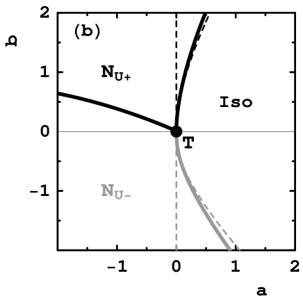
Figure 3: Generic phase diagram with a direct, $N_{U+}-N_{U-}$ first order phase transition. Parameters taken are $c=d=f=1$. For detailed definition of all symbols and lines used see caption to Fig. 2. The triple point (T) is localized at $(a,b)=(0,0)$.

Also in this case the transition line can be given in an analytical form as:

$$a = u\left[2du(d+2fu)+c(2d+5fu)\right]\times$$ (16)

$$\frac{\left[5c+2u(4d+5fu)\right]}{4(d+5fu)^{2}}$$

$$b = -\frac{u\left[3cd+2u\left(3d^{2}+7fud+5f^{2}u^{2}\right)\right]}{2(d+5fu)}$$ (17)

with the free energy

$$F_{u}=-\frac{u^{2}(3d+5fu)\left[5c+2u(4d+5fu)\right]^{3}}{240(d+5fu)^{3}}.$$ (18)

The parameter u must satisfy the inequalities

$$-\frac{3d}{5f} \leq u\leq -\frac{d}{5f}\hskip 14.22636pt\text{for}\hskip 14.22636pt25cf\leq 6d^{2}$$ (19)

$$-\frac{d}{5f} \leq u\leq 0\hskip 29.87538pt\text{for}\hskip 14.22636pt25cf\geq 6d^{2}.$$ (20)

Generally, this topology is observed for the $\frac{cf}{d^{2}}$ parameter taken from outside of the interval $[\frac{6}{25},\frac{9}{25}]$ (see discussion below leading to inequalities (24, 25)) and is the most typical for the uniaxial family of the phase diagrams, Figs. 12-14. The appearance of the ${N_{U+}}-{N_{U-}}$ line is a result of competition between the third- and the fifth order invariants in the free energy expansion when the coefficients weighting these terms are of the opposite sign. For ${25}cf\geq 9d^{2}$ the three phases: $Iso$, $N_{U+}$ and $N_{U-}$ meet at the triple point, T, of coordinates $(a,b)=(0,0)$ where $u=0$ and $F_{u}=0$. At T the lines $Iso-N_{U+}-$ and $Iso-N_{U-}$ have a common tangent given by the $a=0$ line. For ${25}cf\leq 6d^{2}$ the triple point moves away from the origin to a new location at

$$a = \frac{3\left(6d^{2}-25cf\right)^{2}}{10000f^{3}}$$ (21)

$$b = \frac{9d\left(6d^{2}-25cf\right)}{500f^{2}},$$ (22)

which is obtained by substituting $u=-\frac{3d}{5f}$ into Eqs. (16).

III.1.3 Class (c)

This class of the phase diagrams is perhaps the most interesting one among the uniaxial topologies. In addition to the ${N_{U+}}-{N_{U-}}$ transition line, shown in Fig. 3 and given by (16,20), it also displays a direct $N_{U-}-N_{U-}$ first-order phase transition line terminating at a critical point of the liquid-vapor type.

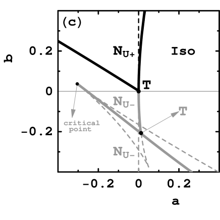
Figure 4: Generic phase diagram with a direct, $N_{U-}-N_{U-}$ first order phase transition terminating at a critical point. Parameters taken are $(c,d,f)=(1,1.05,0.306)$. Note that one of the spinodal lines connected with the $N_{U+}$ phase is separated from the transition line $Iso-N_{U+}$ by less than the thickness of the graph, and, hence, is invisible. For detailed definition of all symbols and lines used see caption to Fig. 2.

Again this behavior results from the aforementioned competition between the third- and the fifth order terms in the free energy expansion. An example of the ${N_{U-}}\leftrightarrow{N_{U-}}$ line, together with the lines: $~{}Iso\leftrightarrow{N_{U-}}$, $~{}Iso\leftrightarrow{N_{U+}}$ and $~{}Iso\leftrightarrow{N_{U+}}\leftrightarrow{N_{U-}}$, is shown in Fig. 4. The lines terminate at the $Iso-N_{U+}-N_{U-}$ triple point of coordinates $(a,b)=(0,0)$ and at the $Iso-N_{U-}-N_{U-}$ triple point given by the formula (21). The necessary condition for this class of the diagrams to appear is a requirement that the spinodal has two cuspidal points for the oblate states ($q<0$). After inspecting $q$-dependence of the curve (11) one easily finds that the $(a,b)$-coordinates of these points are obtained by substituting

$$q_{\pm}=\frac{-d\pm\sqrt{d^{2}-\frac{8}{3}cf}}{4f}$$ (23)

into Eq. (11). Additionally, the conditions $0\leq{8cf}<{3}d^{2}\,\,\,\,\wedge\,\,\,\,c>0$ (in our re-scaling $c=1$) must be met for the cuspidal points with negative values of $q$ to occur. Taken together, these conditions guarantee that there exist two local minima (usually one of them becomes the global one) and two local maxima in the free energy branch for the oblate states ($q<0$). The local minima can finally convert into a stable $N_{U-}-N_{U-}$ line, Eq. (16), if

$${6}{}d^{2}\leq 25{cf}{}\leq{9}{}d^{2}\,\,\,\,\, \wedge \,\,\,\,\,c>0$$ (24)

$$-\frac{d}{2f}-\frac{\sqrt{9d^{2}-24cf}}{6f}\leq u \leq-\frac{3d}{5f}.$$ (25)

Note that the conditions (24,25) are more restrictive than the ones for the cuspidal points of the spinodal. The first one, (24), states that the $Iso-N_{U-}-N_{U-}$ triple point disappears (and hence also the $N_{U-}-N_{U-}$ line) for $b>0$. Additionally, it guarantees the appearance of the $Iso-N_{U-}-N_{U-}$ triple point (cusp) in the $F_{u}(q<0)=0$ branch of the free energy for $b<0$. The second inequality, (25), represents actually the same restrictions, but expressed in terms of u. Finally, coordinates of the critical point are obtained by substituting $q_{-}$, Eq. (23), into Eq. (11). This leads to

$$a = \frac{4cf\left(3d^{2}-2cf\right)-3d^{4}}{96f^{3}}-\frac{d\left(3d^{2}-8cf\right)^{3/2}}{96\sqrt{3}f^{3}}\hskip 8.53581pt$$ (26)

$$b = \frac{9d^{3}-36cfd+\sqrt{3}\left(3d^{2}-8cf\right)^{3/2}}{72f^{2}}.$$ (27)

Sector of stability of the class (c) is shown in Fig. 14. It is restricted to the area given by $6d^{2}/25<f<9d^{2}/25\wedge f<1$. The richest phase sequence obtained for this class as temperature is lowered is $Iso-N_{U+}-N_{U-}-N_{U-}$.

III.1.4 Class (d)

Quite interesting and untypical situation is met when $cf/d^{2}$ approaches one of its two limiting values in (24). For $cf=\frac{6}{25}d^{2}$, Fig. 14, the $N_{U-}-N_{U-}$ transition line and a part of the $N_{U+}-N_{U-}$ transition line become reduced to a common straight line

$$b=-\frac{5f}{2d}\,a,\hskip 28.45274pta\in[-\frac{8d^{4}}{625f^{3}},0].$$ (28)

That is, the $N_{U-}-N_{U-}$ transition line becomes also a line of triple points with the critical and triple point collapsing at $a=-\frac{8d^{4}}{625f^{3}}$! This case, illustrated in Fig. 5, makes us to expect that when higher orders in the expansion (6) are taken into account the degeneracy of the $N_{U-}-N_{U-}-N_{U+}$ line should be removed and replaced by an $(Iso)-N_{U-}-N_{U-}-N_{U+}$ bubble-shaped diagram with up-to three triple points. Bracket indicates that the branch $Iso-N_{U-}$ does not need to be present.

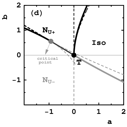
Figure 5: Degenerated version of phase diagram shown in Fig. 4. The $N_{U-}-N_{U-}$ line (together with the critical point) belongs to the $N_{U-}-N_{U+}$ line starting at $a=0$, both being straight lines. The dashed straight line above the critical point is a continuation of the $N_{U-}-N_{U-}$ line and serves as a reference to $N_{U-}-N_{U+}$ line. Parameters taken are $(c,d,f)=(1,1,6/25)$. For detailed definition of all symbols and lines used see caption to Fig. 2.

At $cf=\frac{9}{25}d^{2}$, which is the second of the two limits, the $N_{U-}-N_{U-}$ line becomes reduced to a single critical point located at $(a,b)=(\frac{2d^{4}}{625f^{3}},-\frac{7d^{3}}{125f^{2}})$. The point belongs to the $Iso-N_{U-}$ transition line.

The phase diagrams described so far are stable against formation of the biaxial phase given that $\phi\equiv f-1\leq 0$. If this condition is fulfilled we can always find a uniaxial state with free energy lower than- or equal to the free energy of any biaxial state. Indeed, consider a biaxial phase of $0<\omega<1$. A sufficient condition for the equilibrium value $\omega_{b}$ of $\omega$ in the biaxial phase is then given by

$$\left.\frac{\partial F}{\partial\omega}\right|_{\omega_{b}}=F_{b}(q)+\frac{1}{3}\phi\,q^{6}{\omega_{b}}=0,\hskip 14.22636pt0<\omega_{b}<1,$$ (29)

which, when solved for $F_{b}(q)$ and substituted back to the biaxial free energy formula, Eq. (6), yields

$$F_{biax}\equiv F(q,\omega_{b})=F_{0}+F_{u}(q)-\frac{1}{6}\phi\,q^{6}{\omega_{b}}^{2}.$$ (30)

The Eq. (30) clearly shows that only for $\phi>0$ ($f>1$) there is a chance to get a stable biaxial nematic phase. For $\phi<0$ the uniaxial state is always more favorable. The same conclusions are drawn for the biaxial state of $\omega=1$. By a direct calculation of the free energy we find for this case that the biaxial state of the free energy $F(q=q_{b},\omega=1)$, is always less stable than one of the two uniaxial states: $\{q=\pm q_{b}$, $\omega=0\}$, where $q_{b}$ is value of $q$ in the biaxial phase.

III.2 Phase diagrams with biaxial nematic phase: $q\neq 0,0<\omega\leq 1$

The discussion of the previous section shows that, generally, a stable biaxial nematic phase is found for $\phi=f-e\equiv f-1>0$. In this section we analyze this case more thoroughly. We start by pointing out that the sign of the $F_{b}(q)$ term in Eq. (6) decides about the relative stability of the biaxial order with respect to all other phases involved. Generally, a uniaxial phase becomes unstable against formation of the long-range biaxial order if $F_{b}(q)\leq 0$, which implies that

$$b\,\gtrless\frac{3}{5}\,d\,q^{2}+\phi\,q^{3},\hskip 14.22636ptq\gtrless 0.$$ (31)

In addition, for $F_{b}(q)\leq-\frac{1}{3}\,\phi\,q^{6}$, or, equivalently

$$b\,\lessgtr\frac{3}{5}\,d\,q^{2},\hskip 14.22636ptq\gtrless 0$$ (32)

the phase biaxiality, $\omega$, attains its maximal value $\omega_{b}=1$, Eq. (29). The equality sign in the condition (31) marks a bifurcation from the uniaxial to the biaxial phase. Together with (9), this can be solved for $a$ and $b$ to give the spinodal lines in a parametric form:

$$(a,b)=\left(-cq^{2}-\frac{2d}{5}\,q^{3}-q^{4},\frac{3d}{5}\,q^{2}+\phi\,q^{3}\right).$$ (33)

A few general conclusions can be drawn from the formulas (6,33) and inequality (31). First of all, if Eq. (33) is fulfilled on a globally stable uniaxial nematic branch, the transition $N_{U}-N_{B}$ is second order. Satisfying relation (33) on a locally stable uniaxial branch results in a first order $N_{U}\,(Iso)-N_{B}$ phase transition. That is, the bifurcation scenario allows for a possibility of a tricritical point on the $N_{U}-N_{B}$ line. Second order $Iso-N_{B}$ transition is only admitted to states of maximal biaxiality ($\omega=1$).

For the biaxial branch of the free energy a more quantitative analysis can be given. In particular, the biaxial free energy (30) can be expressed in an equivalent form as

$$F_{biax}=-\frac{b^{2}}{6\phi}+\frac{1}{2}\alpha q^{2}+\frac{1}{4}\gamma q^{4}+\frac{q^{6}}{6},$$ (34)

where

$$\alpha=a+\frac{2bd}{5\phi},\hskip 14.22636pt\gamma=c-\frac{6\,d^{2}}{25\phi}\hskip 11.38109pt\text{and}\hskip 11.38109pt\gamma^{2}\geq 4\alpha.$$ (35)

A convenient parametric form for the $Iso-N_{B}$ line now easily follows from the equation $F_{biax}=0$, supplemented with the condition for $q_{b}$: $(\partial F_{biax}/\partial q)_{q=q_{b}}=0$. The solution of practical importance may be expressed as

$$\left(a=-\frac{2bd}{5\phi}-\gamma q^{2}-q^{4},b^{2}=-\frac{1}{2}q^{4}\left(4q^{2}+3\gamma\right)\phi\right).$$ (36)

Additionally, a stability criterion of the biaxial solution is given by the condition that determinant of second derivatives of the free energy is positive definite. This means that the biaxial phase is locally stable if

$$\frac{\partial^{2}F}{\partial q^{2}}\frac{\partial^{2}F}{\partial\omega^{2}}-\left(\frac{\partial^{2}F}{\partial q\,\partial\omega}\right)^{2}\geq 0\hskip 28.45274pt\Longrightarrow$$

$$4\alpha+\gamma\left(\sqrt{\gamma^{2}-4\alpha}-\gamma\right)>0.$$ (37)

The limiting case of vanishing determinant gives two straight lines in the $(a,b)$-plane: $\left\{\alpha=0,\gamma^{2}=4\alpha\right\}$, which are further spinodals of the model.

Detailed analysis of relative stability of $Iso$, $N_{U}$ and $N_{B}$ phases shows that all ’uniaxial’ phase diagrams, Figs. 2-5, have their biaxial counterparts. Generally, the biaxial phase replaces, at least partly, the $N_{U+}-N_{U-}$ transition line by the two lines: ${N_{U+}}\leftrightarrow{~{}N_{B}}$ and ${N_{U-}}\leftrightarrow{N_{B}}$. They can be given in a parametric form as functions of the real parameter $q_{1}$

$${5\delta a}{} = q_{1}\left[\left(6q^{2}-10q_{1}^{2}\right)d^{2}-10\zeta q_{1}d+\right.$$ (38)

$$\hskip 28.45274pt\left.25q^{2}\left(q^{2}+c\right)\phi\right]$$

$$5\delta b = 6d^{2}q^{2}-25\phi\left[q^{4}-q_{1}^{3}\left(d+fq_{1}\right)+\right.$$ (39)

$$\hskip 28.45274pt\left.c\left(q^{2}-q_{1}^{2}\right)\right]$$

$$50q^{2}\phi = 4d^{2}-40\phi q_{1}d-50\zeta\phi\pm$$ (40)

$$\sqrt{2}\sqrt{\delta^{2}\left(2d^{2}+40\phi q_{1}d+25(2\zeta-c)\phi\right)},$$

with $\delta=2d+5\phi q_{1}$ and $\zeta=fq_{1}^{2}+c$. The parameter $q_{1}$ runs over the uniaxial branches, where $q_{1}>0$ for $N_{U+}$ and $q_{1}<0$ for $N_{U-}$. Analyzing various cases we are able to single out six additional classes of the diagrams, shown in Figs. 6-11, that supplement the uniaxial family. Again, the phase diagrams with the $N_{B}$ phase should be correlated with Figs. 12-14, where sectors of absolute stability of a given class are shown in the $\{c,d,f\}$ parameter space.

The discussion of the biaxial phase diagrams will proceed in a similar way as for the uniaxial case, that is we again start with the case of $d=0$. In this limit we can distinguish between the two different classes of the diagrams, all being symmetric with respect to the $b=0$ line.

III.2.1 Class (e)

The first class, shown in Fig. 6, is similar to (a), Fig. 2.

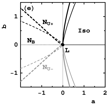
Figure 6: Generic phase diagram for $d=0$ and $c\geq 0$. Biaxial phase is sandwiched between two uniaxial phases. A direct phase transition from the isotropic phase to biaxial nematic is possible through the Landau point. Solid lines represent phase transitions of first order, dashed lines second order. Two cases are shown: $c=0,d=0,f=1.5$ (thin lines) and $c=1,d=0,f=1.5$ (thick lines). As previously, gray lines represent phase transitions involving $N_{U-}$ phase.

The only difference is that the line separating ${N_{U+}}$ and ${N_{U-}}$ splits itself into ${N_{U+}}\leftrightarrow{~{}N_{B}}$ and ${N_{U-}}\leftrightarrow{N_{B}}$ lines of second order phase transitions with $N_{B}$ phase positioned in between. We find this class stable for $c\geq 0$ and $f>1(\equiv\phi>0)$. As previously the uniaxial lines are given by (15). For the ${N_{U}}-{~{}N_{B}}$ lines the formulas (38) now simplify to

$$b^{2}=\frac{1}{2}\left(3ac-c^{3}+\sqrt{c^{2}-4a}\left(c^{2}-a\right)\right)\phi^{2},$$ (41)

where $a\leq 0$. The four phases: $~{}Iso$, ${N_{U+}}$, ${N_{B}}$ and ${N_{U-}}$ meet at the Landau (tetracritical) point: $L=(a,b)=(0,0)$. Additionally, for $c=0$ the ${N_{U+}}-{~{}N_{B}}$ and ${N_{U-}}-{~{}N_{B}}$ lines have a common tangent at L, which is given by the $a=0$-line. For $c=1$ this tangent is the $b=0$-line.

III.2.2 Class (f)

The diagrams of this class, Fig. 7, are also derived from (a) and observed when $c<0$.

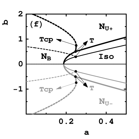
Figure 7: Generic phase diagram for $d=0$ and $c<0$. Biaxial phase becomes stable between two uniaxial phases. A direct phase transition from isotropic phase to biaxial nematic is possible along the line between the two triple points, T, that replace the Landau point. Solid lines represent phase transitions of first order, dashed lines second order. Tcp stands for tricritical point. Two cases with $f\lessgtr 2$ are shown: $c=-1,d=0,f=1.7$ (thin lines) and $c=1,d=0,f=3.1$ (thick lines). For the meaning of lines see caption to Fig. 6.

Again the uniaxial lines are given by Eq. (15) and the ${N_{U}}-{~{}N_{B}}$ lines by Eq. (41). The latter represent thermodynamically stable, second-order transition lines if

$$a \leq \frac{3c^{2}(2f-1)}{4(f+1)^{2}}\hskip 14.22636pt\text{for}\hskip 14.22636pt1<f\leq 2$$ (42)

$$a \leq \frac{c^{2}}{4}\hskip 54.06023pt\text{for}\hskip 14.22636ptf>2.$$ (43)

A new feature shown is a splitting of the Landau point into two triple points where $Iso$, $N_{U}$ and $N_{B}$ meet. The position of the triple points is

$$(a,b^{2}) = \left(\frac{3c^{2}(2f-1)}{4(f+1)^{2}},-\frac{27c^{3}(f-1)^{2}}{8(f+1)^{3}}\right).$$ (44)

Both triple points are connected by a direct $Iso\leftrightarrow{N_{B}}$ line of first order phase transitions for which we have

$$b^{2}=\frac{1}{4}\phi\left[c\left(c^{2}-6a\right)-\left(c^{2}-4a\right)^{3/2}\right].$$ (45)

Depending on $f$, the phase transition between $N_{U}$ and $N_{B}$ can be either first or second order. For $1\leq f\leq 2$ only second order $N_{U}-N_{B}$ transitions are realized. For $f>2$ the second order transition line (41) is separated from the triple point by the ${N_{U}}-{~{}N_{B}}$ line of first order phase transitions ($\omega\neq 0$). Both ${N_{U}}-{~{}N_{B}}$ lines meet at the tricritical point given by

$$(a,b^{2})=\left(\frac{c^{2}}{4},-\frac{1}{8}c^{3}\phi^{2}\right).$$ (46)

III.2.3 Class (f’)

Now we turn to a more complex case, namely that of $d\neq 0$. It is quite convenient to discuss new features of the diagrams that emerge in this case by referring directly to the parameter space division as shown in Figs. 12-14. New classes will be parameterized by $c=\pm 1,0$. It turns out that for $c=-1$, the effect of nonzero $d$ is merely to distort the phase diagrams classified as (f). The distorted diagrams that preserve all features of (f) are separated from the new class (f’), Fig. 8, by curves:

$$d^{2}=\frac{25c\left(\sqrt{\phi}-1\right)^{2}\phi}{6\left(\phi-2\sqrt{\phi}-2\right)},\hskip 8.53581pt0\leq\phi\leq 4+2\sqrt{3}.$$ (47)

The curves are pictured dark-gray in Fig. 12.

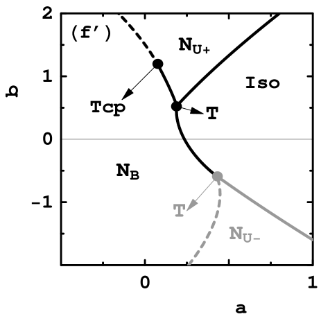
Figure 8: Generic phase diagram for $d\neq 0$ and $c<0$. Biaxial phase becomes stable between two uniaxial phases. A direct phase transition from the isotropic phase to biaxial nematic is possible along the line between two triple points (T) that replace the Landau point. Only one tricritical point (Tcp), along $N_{U+}-N_{B}$, is possible for this class of diagrams. Parameters taken are: $c=-1,d=1,f=3$. For the meaning of lines see caption to Fig. 6.

The area to the right, shown as light-gray, represents the class (f’). The class differs from the deformed versions of (f-Tcp)-like diagrams with two tricritical points and of (f) without tricritical points by the presence of one tricritical point on the $N_{U+}-N_{B}$ transition line.

III.2.4 Class (g)

The case $c=0$, Fig. 13, results in a new class of the diagrams shown in Fig. 9.

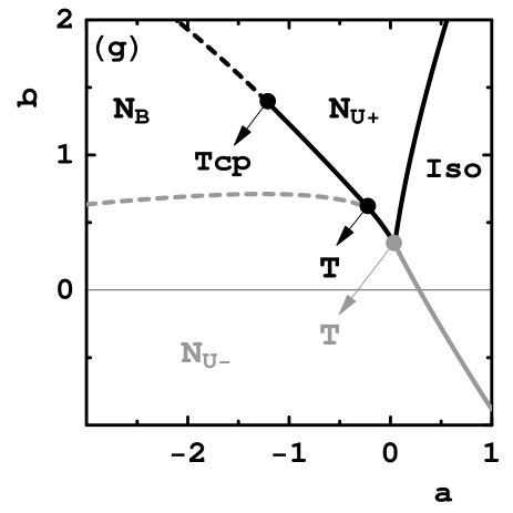
Figure 9: Generic phase diagram for $d\neq 0$ and $c=0$. Biaxial phase becomes stable between two uniaxial phases. A direct phase transition from isotropic phase to biaxial nematic is not possible. Two triple points (T) are connected by the $N_{U+}-N_{U-}$ line of first order phase transitions. One tricritical point (Tcp) appears on the $N_{U+}-N_{B}$ line. Maximum along $N_{U-}-N_{B}$ allows for two biaxial nematic phases on the temperature scale, separated by the $N_{U-}$ phase. The low-temperature biaxial phase is referred to as reentrant $N_{B}$. Parameters taken are: $c=0,d=2,f=1.6$. For the meaning of lines see caption to Fig. 6.

One of the differences between (g) and (f’), exemplified in Fig. 9, is the absence of the direct transition between $Iso$ and $N_{B}$. The $N_{B}$ phase branches off the $N_{U+}-N_{U-}$ first-order transition line at the $N_{U+}-N_{B}-N_{U-}$ triple point. Interestingly, we observe a maximum along the second-order $N_{B}-N_{U-}$ transition line at the location given by

$$(a,b)=\left(\frac{16d^{4}(\phi-1)}{625\phi^{4}},\frac{4d^{3}}{125\phi^{2}}\right).$$ (48)

This maximum indicates that we can observe reentrant biaxial nematic phase as temperature is lowered. Consequently, it leads to a very rich sequence of phase transitions, e.g. $Iso-N_{U+}-N_{B}-N_{U-}-N_{B}$. The reentrant phase and hence also the maximum disappear for $f\geq 2$. In the interval $2<f<1+2/\sqrt{3}$, shown as sector (g’) in Fig. 13, the remaining features of the diagram, Fig. 9, are left unchanged.

III.2.5 Class (h)

For $c=1$ we identify two new classes of the diagrams, denoted (h) and (i). The class (h), Fig. 10, is derived from (e), the difference again being the presence of maximum along the second-order $N_{B}-N_{U-}$ transition line at $(a,b)$ given by Eq. (48).

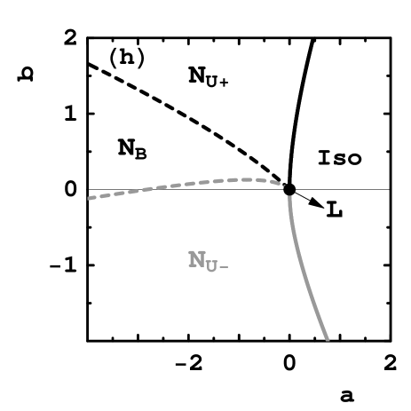
Figure 10: Generic phase diagram for $d\neq 0$ and $c=1$. This class of the diagrams is a deformed versions of (e). A major difference between (e) and (h) is a maximum along $N_{U-}-N_{B}$ that allows for reentrant $N_{B}$. Parameters taken are: $c=1,d=1,f=1.5$. For the meaning of lines and of reentrant $N_{B}$ see captions to Figs. 6 and 9, respectively.

That is we again can observe a sequence of phases with reentrant biaxial nematic. Sector (h), Fig. 14, is separated from the neighboring sectors (g) and (h+c) by the following lines: the dashed one given by $f=1+6d^{2}/25$ ($0\leq d\leq 5/\sqrt{3}$) and the continuous one given by $f=9d^{2}/25$ ($d>5/\sqrt{3}$).

III.2.6 Class (i)

This class of the diagrams is essentially a combination of (g) and (c) and yields the richest sequences of phases and of corresponding phase transitions. They include reentrant biaxial nematic, $N_{U+}-N_{B}$ tricritical point and a line of phase transitions between identical uniaxial phases terminating at a critical point. Exemplary phase diagram is given in Fig. 11.

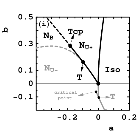
Figure 11: Generic phase diagram for $d\neq 0$ and $c=1$. It combines properties of (g) and (c). Parameters taken are: $c=1,d=3,f=2.75$.

Sector of stability for this class, denoted (i) in Fig. 14, is limited by the following curves: $f=1+6d^{2}/25$ ($d>5/\sqrt{3}$), $f=9d^{2}/25$ ($5/3\leq d\leq 5/\sqrt{3}$), $f=1$ ($5/3\leq d\leq 5/\sqrt{6}$) and $f=6d^{2}/25$ ($d>5/\sqrt{6}$). In a small sector, named (h+c), the tricritical point and the $N_{U+}-N_{U-}$ line disappear, the resulting phase diagrams being a combination of (h) and (c).

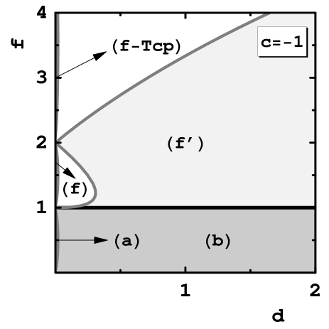
Figure 12: Sectors, in $\{c=-1,d,f\}$ parameter space, of absolute stability of phase diagrams labeled from (a) through (i). (f-Tcp) stands for (f)-class with two tricritical points, Fig. 7. Deformed versions of (f) and (f-Tcp) diagrams are realized within sectors marked white.

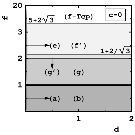
Figure 13: Sectors, in $\{c=0,d,f\}$ parameter space, of absolute stability of phase diagrams labeled from (a) through (i). (g’) stands for (g)-class without reentrant $N_{B}$ (i.e. without a maximum along $N_{U-}-N_{B}$).

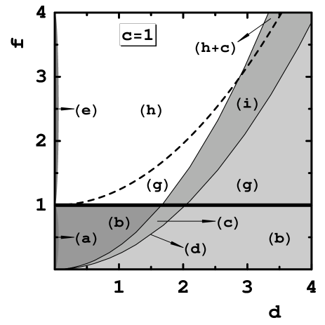
Figure 14: Sectors, in $\{c=1,d,f\}$ parameter space, of absolute stability of phase diagrams labeled from (a) through (i). (h+c) stands for diagrams that combine properties of (h) and (c) (see Figs. 4,10).

III.3 Degenerated phase diagrams for b=0

This case requires a few comments for not all phase sequences with b=0 can be identified from the diagrams that we have given so far. There are also subtle symmetry issues due to the presence of accidental degeneracy.

The identification of phases and of phase sequences for $b=0$ is straightforward for $d\neq 0$, in which case they follow directly from the diagrams representing classes (b,c,d,f’,g,h). Only the case $d=0$, represented by the diagrams (a,e,f), requires separate comments. By inspecting the free energy expansion (6) for $b=d=0$ we find immediately that only three states can be realized at equilibrium: (i) degenerated uniaxial state of $\omega=0$ for $f<1$; (ii) degenerated biaxial-uniaxial state of arbitrary $\omega$ for $f=1$, and (iii) biaxial state of maximal biaxiality ($\omega=1$) for $f>0$.

The uniaxial state, denoted (i), has the same free energy for oblate and prolate states, which means that the system creates oblate and prolate domains with the same energy cost. Due to this accidental degeneracy the symmetry group of the state can be classified as ${\cal{D}}_{\infty h}\times{\cal{Z}}_{2}$. Consequently, the transition from the isotropic phase to the degenerated uniaxial phase can be either second-order ($c=1$) or first order ($c=-1$) with a tricritical point at $c=0$. The transition temperature and the order parameter for temperatures below the transition are given by $\{a=0$ for $c=0,1$; $a=\frac{3}{16f}$ for $c=-1\}$ and $q^{2}=\frac{\sqrt{c^{2}-4af}-c}{2f}$, respectively.

The states (ii,iii) have mathematically the same form of the free energy as one for the degenerated uniaxial case. All formulas are reproduced from the case (i) if we substitute $f=1$ there. Hence, again, the phase transition from the isotropic phase to the corresponding ordered phase can be either first or second order with an intermediate tricritical point. The difference between the cases (ii) and (iii) is in symmetry. For (ii) the only restriction on $\mathbf{Q}$ is $\mathrm{Tr}{(\mathbf{Q}}^{2})=const$. The accidental degeneracy of the equilibrium solutions for $\mathbf{Q}$ is the rotational invariance in five-dimensional space of components $Q_{\alpha\beta}$. The relevant symmetry group is thus ${\cal{O}}({5})$, which seizes up the difference between uniaxial and biaxial domains. We call it the degenerated biaxial-uniaxial phase.

In the case (iii) the tensor $\mathbf{Q}$ is given by Eq. (1) with e.g. $q_{0}=0$, that is by one of the three degenerated solutions fulfilling maximal biaxiality condition $\mathrm{Tr}{(\mathbf{Q}}^{3})=0$.

IV Discussion

The Landau-deGennes theory of biaxial nematics presented in this paper has been elaborated to show the outcome of mathematical structure of the expansion that is based solely on the order parameter $\mathbf{Q}$. The phenomenological approach is particularly simple and the knowledge of full spectrum of predictions of one of the most commonly cited theories is desirable, particularly because of current interest in seeking for stable thermotropic biaxial nematic phase. The analytical formulas are given for almost all transition lines, characteristic points of the lines, and for the stability range of a given class of the phase diagrams. Except for the purely uniaxial group of the diagrams for $f<1$, the biaxial phase is naturally stabilized between prolate and oblate uniaxial nematics. Phase transitions to the biaxial phase can be either first or second order with a possibility of a tricritical point. Due to a competition between cubic and fifth-order invariants the direct $N_{U-}-N_{U-}$, $N_{U+}-N_{U-}$ and the reentrant biaxial nematic phase are also possible. The Landau $Iso-N_{U+}-N_{B}-N_{U-}$ (tetracritical) point can split into two triple points positioned either on the $Iso-N_{B}$ transition line or on the $N_{U+}-N_{U-}$ line.

One may wonder then why the biaxial nematic phase is so difficult to account for experimentally. The practical difficulty could be that for real systems the parameter $f$, responsible for the stabilization of the biaxial nematic phase, is much too small compared to other coefficients of the Landau expansion, so we effectively stay in the uniaxial sector of the diagrams ($f\leq 1$). An alternative explanation could be that smectic and crystalline phases, not taken into account, may interfere before the right thermodynamic parameters are reached. Clearly, the best choice of the Landau coefficients to get $N_{B}$ absolutely stable would be that where $N_{B}$ bifurcates directly from the isotropic phase. At microscopic level it would then be of interest to construct molecular models showing generic types of the diagrams identified phenomenologically. To this goal it is necessary to establish a bridge between molecular and phenomenological approaches, in particular one needs a molecular interpretation of the alignment tensor and, at least, of the $(a,b)$-parameters entering the expansion. The problem is relatively simple in the mean-field approximation and the solution has already been given Mulder (1989); Longa and Paja̧k (2005) for the class of the so called $L=2$ models with ${\cal{D}}_{2h}$-symmetric hard molecules/soft interactions Mulder (1989); Longa et al. (2005). Applying formulas (14-20) from Longa and Paja̧k (2005) to the mean-field versions of the models Alben (1973); Luckhurst and Romano (1980); Sonnet et al. (2003); Longa et al. (2005, 2007); Bates (2006) we recover diagrams represented by (e) Alben (1973); Luckhurst and Romano (1980); Longa et al. (2007), (f) Sonnet et al. (2003); Longa et al. (2005) and (g) Bates (2006). Evidence for degenerated states ($b=d=0$) has been given by Matteis and Virga Matteis and Virga (2005).