Constraining the nature of High Frequency Peakers

Abstract

Aims. The “bright” High Frequency Peakers (HFPs) sample is a mixture of blazars and intrinsically small and young radio sources. We investigate the polarimetric characteristics of 45 High Frequency Peakers, from the “bright” HFP sample, in order to have a deeper knowledge of the nature of each object, and to construct a sample made of genuine young radio sources only.

Methods. Simultaneous VLA observations carried out at 22.2, 15.3, 8.4 and 5.0 GHz, together with the information at 1.4 GHz provided by the NVSS at an earlier epoch, have been used to study the linearly polarized emission.

Results. From the analysis of the polarimetric properties of the 45 sources we find that 26 (58%) are polarized at least at one frequency, while 17 (38%) are completely unpolarized at all frequencies. We find a correlation between fractional polarization and the total intensity variability. We confirm that there is a clear distinction between the polarization properties of galaxies and quasars: 17 (66%) quasars are highly polarized, while all the 9 galaxies are either unpolarized ($<0.2\%$) or marginally polarized with fractional polarization below 1%. This suggests that most HFP candidates identified with quasars are likely to represent a radio source population different from young radio objects.

1 Introduction

From our previous works (Orienti et al. mo06 (2006); Orienti, Dallacasa & Stanghellini mo07 (2007), hereafter Paper I) it is clear that the bright HFP sample (Dallacasa et al. dd00 (2000)) contains both young radio sources and blazars, since it was selected on the basis of single epoch multi-frequency radio observations. It is thus important to properly discriminate/classify these sources on the basis of their intrinsic nature by using all the evidence coming from observations.
The evolutionary stage of a powerful radio source in radio-loud Active Galactic Nuclei can be determined by its linear size. Following a self-similar evolution model (e.g. Fanti et al. cf95 (1995); Readhead et al. read96 (1996); Snellen et al. sn00 (2000)), the most compact sources would evolve into the extended radio galaxy population and eventually into the “oldest” and “largest” sources in the Universe, the class of giant radio galaxies.
However, it has also been claimed (Alexander alexander00 (2000); Marecki et al. ma03 (2003)) that a fraction of young and compact radio sources would die in an early stage, never becoming large-scale objects.
In this scheme the youngest objects are the “Compact Symmetric Objects” (CSOs), which are small ($<$ 1 kpc) radio sources with a convex synchrotron radio spectrum which peaks at frequencies ranging from a few hundred MHz to a few GHz (Wilkinson et al. wil94 (1994)).
Statistical studies of different samples of this class of objects (O’Dea & Baum odea97 (1997)) have led to the discovery of an anti-correlation between the spectral peak and the linear size (i.e. the age): the higher the turnover frequency, the younger (smaller) the source is.
“High Frequency Peaker” (HFP) radio sources (Dallacasa dd03 (2003)), characterized by the same properties of the CSOs, but with observed spectral peaks above 5 GHz, are the best candidates to be newly born radio sources with typical ages of 10² - 10³ years.
So far, the “bright” HFP sample (Dallacasa et al. dd00 (2000)) is the only existing sample of this class of sources. Its selection was based on radio spectral characteristics only.
Other kinds of radio sources, such as blazars, can temporarily match the selection criteria during a phase of their variability, i.e. when a flaring, self-absorbed component at the jet base dominates the radio emission, and thus, they could contaminate a sample selected on the basis of spectral properties. However, genuine young radio sources and blazars show different characteristics, if proper observables are considered. The spectral variability (Tinti et al. st05 (2005); Paper I) and the morphology (Orienti et al. mo06 (2006)) of young HFP candidates have been discussed in earlier works. This paper focuses on the polarimetric properties of these two classes of objects.
Given their intrinsically small linear sizes, young radio sources entirely reside within the Narrow Line Region (NLR) of the host galaxy. The ambient medium of this region is generally described by a two-phase plasma: a component in the form of clumps/clouds, with high density n_e $\sim$ 10⁴ cm^-3 and temperature T $\sim$ 10⁴ K, but a small filling factor (i.e. they occupy about $<$10^-4 of the total volume of the NLR, McCarthy mac93 (1993)); and a diffuse, less dense (n_e $\sim$ 10^-3 cm^-3), and hotter (T $\sim$ 10⁷ K) component, which fills the inter-cloud space. In the presence of a magnetic field, both components can act as a Faraday screen, causing significant Faraday rotation and possibly depolarization of the synchrotron radiation.
Radio sources completely embedded in such an environment are expected to show high Rotation measures (RM) and strong depolarization (DP), if the structure of the Faraday Screen is not resolved, which is generally the case, at least with arcsecond-scale resolution polarimetric observations.
As the source expands ($>$ 1 kpc), its radio emission emerges from the NLR and reaches the outer regions of the host galaxy interstellar medium (ISM) where a more homogeneous environment with less ionization and a weaker magnetic field may substantially reduce the aforementioned effects.
Evidence of a relationship between the fractional polarization and the linear size has been pinpointed by Cotton et al. (cotton03 (2003)) and Fanti et al. (cf04 (2004)) by studying samples of compact steep spectrum (CSS) and GHz-peaked spectrum (GPS) radio sources spanning linear sizes from a fraction to a few kpc. In their work, Cotton et al. (cotton03 (2003)) found that at 1.4 GHz almost all the sources smaller than 6 kpc are completely unpolarized. At higher frequencies (i.e. 5.0 and 8.4 GHz), Fanti et al. (cf04 (2004)) found a similar effect but the complete depolarization of the radiation progressively happens at smaller linear sizes ($<$ 3-5 kpc).
Similar results have been obtained by Stanghellini et al. (cs98 (1998)) on a sample of GPS sources, whose typical linear size is $<$ 1 kpc. They found that the majority of the GPS objects have very low fractional polarization, with upper limits consistent with the residual instrumental polarization.
On the other hand, blazars are usually large radio sources, but they appear compact since their size is foreshortened by projection together with some amount of beaming that enhances the emission of the core region and jet base, making the large scale, low-surface brightness emission barely visible in low dynamic range observations. In the unified scheme (e.g. Antonucci anto93 (1993); Urry & Padovani urry95 (1995)), blazars are thought to be oriented at small angles to the line of sight, allowing us to see their nuclear radiation directly and not through the magneto-ionic medium and the obscuring torus. For this reason they are expected to be significantly polarized, as is usually found (e.g. Saikia saikia99 (1999)). However, the high polarization shown by these objects may also be due to Doppler boosted knots in jets, as may be the case in 3C 351 (Saikia saikia99 (1999)).
In this paper we present polarimetric data of 45 HFP candidates from the “bright” HFP sample (Dallacasa et al. dd00 (2000)) observed with the VLA at frequencies from 4.6 to 22 GHz.

2 Polarization observations and data reduction

Simultaneous multi-frequency observations of 45 (out of 55) HFPs that were visible during the allocated observing time were carried out in July 2002 with the VLA in B configuration, in full polarization. The observing bandwidth was chosen to be 50 MHz per IF. A separate analysis for each IF in L, C and X bands was carried out to improve the spectral coverage of the data, as was done in previous works (Dallacasa et al. dd00 (2000); Tinti et al. st05 (2005)).
We obtained the flux density measurements in the L band (IFs at 1.465 and 1.665 GHz), C band (4.565 and 4.935 GHz), X band (8.085 and 8.465 GHz), U band (14.940 GHz) and K band (22.460 GHz).
Each source typically was observed for 60 seconds in each band, cycling through frequencies. Therefore, the flux density measurements can be considered simultaneous.
Since the sources are relatively strong with small angular sizes, the snap-shot observing mode was considered adequate. For each frequency about 3 min were spent on each primary flux density calibrator 3C 286 and 3C 48. Secondary calibrators, chosen to minimize the telescope slewing time, were observed for 1.5 minutes at each frequency every 25 minutes. An appropriate calibrator (J1927+739) for the instrumental polarization was observed over a wide range of parallactic angles.
The data reduction followed the standard procedures for the VLA, implemented in the NRAO AIPS software.
After the standard amplitude and phase calibration, the instrumental polarization was determined and removed. The absolute orientation of the electric vector was determined from the data of the primary flux density calibrator 3C 286, which was observed twice. The residual instrumental polarization is conservatively evaluated to be 0.1%-0.3%, and an uncertainty on the orientation of about 2^∘-3^∘, depending on the observing bands, being worse in U and K bands.
Total intensity data at all frequencies, together with the analysis of the spectral variability have been published by Tinti et al. (st05 (2005)).
Our measurements in the L band are less sensitive than those from the NVSS (Condon et al. condon98 (1998)) due to a less accurate calibration of the instrumental polarization, mainly caused by some radio frequency interferences (RFI) which affected some scans of the calibrator of the instrumental polarization. We then complemented our data with the polarization measurements available from the NVSS, in order to compare our sample with the results by Cotton et al. (cotton03 (2003)) and Fanti et al. (cf04 (2004)).
Polarization images in the Stokes’ U and Q parameters were produced for each frequency, with the exception of the L band.

Table 1: Polarization properties. Col. 1: source name (J2000); Col. 2: optical identification (Table 2) Col. 3: redshift; Col. 4: pc-scale morphology (see Table 2) Col. 5, 7, 9, 12, 15: polarization percentage $m$ and the error $\sigma_{m}$ in K, U, X, C and L bands respectively; Col. 6, 8, 10, 11, 13, 14, 16: polarization angle $\chi$ and the error $\sigma_{\chi}$ in K, U, X, C and L bands.

Source	Id.	z	Morph.	mK	$\chi^{K}$	mU	$\chi^{U}$	mX	$\chi^{X}_{\rm 1}$	$\chi^{X}_{\rm 2}$	mC	$\chi^{C}_{\rm 1}$	$\chi^{C}_{\rm 2}$	mL	$\chi^{L}$
(1)	(2)	(3)	(4)	(5)	(6)	(7)	(8)	(9)	(10)	(11)	(12)	(13)	(14)	(15)	(16)
J0003+2129	G	0.452	CSO	0.7$\pm$0.4	-35$\pm$11	0.6$\pm$0.4	16$\pm$10	$<$0.2	-	-	$<$0.2	-	-	$<$0.1	-
J0005+0524	Q	1.887	CSO	-	-	-	-	0.5$\pm$0.3	15$\pm$4	37$\pm$6	$<$0.2	-	-	$<$0.3	-
J0037+0808	EF		CSO	$<$0.3	-	$<$0.3	-	$<$0.2	-	-	$<$0.2	-	-	$<$0.5	-
J0111+3906	G	0.668	CSO	$<$0.1	-	$<$0.1	-	$<$0.1	-	-	$<$0.1	-	-	$<$0.1	-
J0116+2422	EF		Un	$<$0.3	-	-	-	$<$0.2	-	-	$<$0.2	-	-	0.4	-
J0217+0144	Q	1.715	Un	1.0$\pm$0.1	71$\pm$3	2.2$\pm$0.1	73$\pm$3	2.7$\pm$0.1	87$\pm$2	87.3$\pm$2	1.7$\pm$0.1	83$\pm$2	90$\pm$2	1.5$\pm$0.1	42$\pm$1.0
J0329+3510	Q	0.5	CJ	1.6$\pm$0.2	-1$\pm$3	1.6$\pm$0.1	35$\pm$3	0.5$\pm$0.1	59$\pm$3	44$\pm$3	1.0$\pm$0.1	-75$\pm$2	-73$\pm$2	5.0$\pm$0.3	-46$\pm$1
J0357+2319	Q		Un	3.2$\pm$0.3	88$\pm$3	2.2$\pm$0.3	-87$\pm$4	1.7$\pm$0.4	-80$\pm$3	-78$\pm$3	1.5$\pm$0.4	-68$\pm$3	-80$\pm$3	0.8$\pm$0.3	-16$\pm$6
J0428+3259	G	0.479	CSO	$<$0.2	-	$<$0.1	-	$<$0.1	-	-	$<$0.1	-	-	$<$0.3	-
J0519+0848	EF		Un	1.6$\pm$0.2	55$\pm$3	-	-	1.0$\pm$0.1	-89$\pm$2	89$\pm$3	2.0$\pm$0.1	86$\pm$2	85$\pm$2	2.3$\pm$0.3	-6$\pm$2
J0625+4440	BL		Un	0.7$\pm$0.2	-75$\pm$5	-	-	2.1$\pm$0.2	-87$\pm$3	-86$\pm$2	2.4$\pm$0.2	-86$\pm$3	-86$\pm$2	4.7$\pm$0.4	-79$\pm$1
J0638+5933	EF		CSO	$<$0.1	-	-	-	$<$0.1	-	-	$<$0.1	-	-	$<$0.2	-
J0642+6758	Q	3.180	Un	$<$0.3	-	0.8$\pm$0.2	-43$\pm$6	0.6$\pm$0.1	-69$\pm$3	-60$\pm$3	1.6$\pm$0.1	-81$\pm$2	-84$\pm$2	$<$0.2	-
J0646+4451	Q	3.396	MR	2.5$\pm$0.2	19$\pm$3	3.6$\pm$0.1	17$\pm$3	3.1$\pm$0.1	30$\pm$2	28$\pm$2	1.6$\pm$0.1	29$\pm$2	31$\pm$2	0.8$\pm$0.1	44$\pm$2
J0650+6001	Q	0.455	CSO	$<$0.1	-	-	-	$<$0.1	-	-	$<$0.1	-	-	$<$0.1	-
J1335+4542	Q	2.449	CSO	$<$0.2	-	-	-	$<$0.1	-	-	$<$0.1	-	-	$<$0.2	-
J1335+5844	EF	-	CSO	$<$0.2	-	-	-	$<$0.1	-	-	$<$0.1	-	-	$<$0.1	-
J1407+2827	G	0.0769	CSO	$<0.2$	-	-	-	$<$0.2	-	-	$<$0.1	-	-	$<$0.1	-
J1412+1334	EF		Un	$<$0.3	-	-	-	$<$0.2	-	-	$<$0.1	-	-	$<$0.4	-
J1424+2256	Q	3.626	Un	-	-	-	-	3.4$\pm$0.1	3$\pm$2	3$\pm$2	0.4$\pm$0.1	62$\pm$3	-89$\pm$3	0.6$\pm$0.2	3$\pm$5
J1430+1043	Q	1.710	MR	-	-	-	-	$<$0.1	-	-	$<$0.1	-	-	0.5$\pm$0.2	-71$\pm$6
J1457+0749	BL		Un	-	-	2.8$\pm$0.3	-39$\pm$4	5.3$\pm$0.1	-35$\pm$2	-37$\pm$2	5.7$\pm$0.2	-33$\pm$2	-34$\pm$2	-	-
J1505+0326	Q	0.411	Un	1.1$\pm$0.1	-43$\pm$3	-	-	0.7$\pm$0.1	-45$\pm$3	-44$\pm$3	0.2$\pm$0.1	-41$\pm$3	-45$\pm$3	1.6$\pm$0.1	56$\pm$1
J1511+0518	G	0.084	CSO	$<$0.1	-	-	-	$<$0.1	-	-	$<$0.1	-	-	$<$0.7	-
J1526+6650	Q	3.02	MR	$<$0.4	-	$<$0.3	-	$<$0.1	-	-	$<$0.1	-	-	$<$0.6	-
J1603+1105	BL		Un	$<$0.2	-	$<$0.3	-	0.9$\pm$0.2	-39$\pm$3	-36$\pm$3	1.8$\pm$0.2	-3$\pm$3	-6$\pm$3	-	-
J1616+0459	Q	3.197	CJ	2.3$\pm$0.2	90$\pm$4	-	-	2.9$\pm$0.1	-86$\pm$3	84$\pm$3	0.4$\pm$0.1	-41$\pm$3	-66$\pm$3	$<$0.2	-
J1623+6624	G	0.203	Un	$<$0.3	-	$<$0.2	-	$<$0.2	-	-	$<$0.2	-	-	$<$0.3	-
J1645+6330	Q	2.379	Un	2.9$\pm$0.3	78$\pm$3	2.7$\pm$0.1	73$\pm$3	3.0$\pm$0.1	63$\pm$3	64$\pm$3	1.3$\pm$0.1	46$\pm$2	45$\pm$2	2.4$\pm$0.2	-15$\pm$2
J1735+5049	G		CSO	$<$0.1	-	$<$0.1	-	$<$0.1	-	-	$<$0.1	-	-	$<$0.1	-
J1800+3848	Q	2.092	Un	0.6$\pm$0.1	-84$\pm$3	-	-	0.3$\pm$0.1	-62$\pm$3	-24$\pm$3	$<$0.1	-	-	0.6$\pm$0.1	56$\pm$5
J1811+1704	BL		CJ	7.1$\pm$0.7	-50$\pm$3	6.7$\pm$0.3	-42$\pm$3	1.8$\pm$0.1	12$\pm$3	9$\pm$3	2.3$\pm$0.1	-19$\pm$3	-27$\pm$3	-	-
J1840+3900	Q	3.095	Un	1.0$\pm$0.4	85$\pm$8	-	-	$<$0.3	-	-	$<$0.3	-	-	$<$0.4	-
J1850+2825	Q	2.560	MR	$<$0.1	-	$<$0.1	-	$<$0.1	-	-	$<$0.1	-	-	$<$0.3	-
J1855+3742	G		CSO	$<$0.4	-	$<$0.4	-	$<$0.2	-	-	$<$0.1	-	-	$<$0.3	-
J2021+0515	Q		CJ	1.6$\pm$0.2	47$\pm$4	1.4$\pm$0.2	-76$\pm$4	$<$0.1	-	-	$<$0.3$\pm$0.1	-	-	$<$0.3	-
J2024+1718	Q	1.05	Un	0.9$\pm$0.1	45$\pm$3	0.6$\pm$0.1	-32$\pm$4	0.8$\pm$0.1	45$\pm$3	45$\pm$3	0.2$\pm$0.1	-2$\pm$3	-5$\pm$3	$<$0.3	-
J2101+0341	Q	1.013	Un	2.5$\pm$0.1	-68$\pm$3	3.5$\pm$0.1	-69$\pm$3	4.5$\pm$0.1	-70$\pm$2	-68$\pm$2	3.7$\pm$0.1	-58$\pm$2	-60$\pm$2	$<$0.1	-
J2123+0535	Q	1.878	CJ	3.7$\pm$0.2	-1$\pm$3	2.7$\pm$0.1	1$\pm$3	0.8$\pm$0.1	22$\pm$3	15$\pm$3	1.1$\pm$0.1	82$\pm$3	82$\pm$3	2.0$\pm$0.1	53$\pm$1
J2203+1007	G		CSO	$<$0.4	-	$<$0.4	-	$<$0.2	-	-	$<$0.2	-	-	$<$0.4	-
J2207+1652	Q	1.64	Un	$<$0.3	-	$<$0.3	-	1.5$\pm$0.2	85$\pm$3	87$\pm$3	1.3$\pm$0.2	-72$\pm$3	-80$\pm$3	3.6$\pm$0.2	55$\pm$1
J2212+2355	Q	1.125	Un	8.6$\pm$0.4	36$\pm$3	7.9$\pm$0.4	38$\pm$3	6.8$\pm$0.2	28$\pm$2	28$\pm$2	5.7$\pm$0.2	-4$\pm$2	1$\pm$2	2.0$\pm$0.1	43$\pm$1
J2257+0243	Q	2.081	Un	$<$0.2	-	$<$0.2	-	$<$0.3	-	-	$<$0.1	-	-	0.9$\pm$0.2	44$\pm$1
J2320+0513	Q	0.622	Un	0.9$\pm$0.1	69$\pm$3	1.3$\pm$0.1	44$\pm$3	2.7$\pm$0.1	59$\pm$2	58$\pm$2	4.3$\pm$0.1	71$\pm$2	71$\pm$2	2.3$\pm$0.1	59$\pm$1
J2330+3348	Q	1.809	MR	1.1$\pm$0.1	44$\pm$3	$<$0.2	-	0.5$\pm$0.1	-33$\pm$3	-33$\pm$3	1.4$\pm$0.1	-17$\pm$3	-15$\pm$3	1.2$\pm$0.2	-39$\pm$4

The final noise (1$\sigma$) is usually of $\sim$ 0.07 mJy/beam for C and X bands, and $\sim$ 0.2 mJy/beam for U and K bands, although for a few objects a higher noise level was found in these latter bands, limiting the sensitivity in detect-polarized emission.
Images of the polarization intensity, polarization angle and percentage polarization were produced for all the sources.
Based on the Stokes’ parameters and their errors the polarization parameters were calculated for each frequency as in Klein et al. (uk03 (2003)).
Polarization percentage and polarization angle with their errors at each frequency are reported in Table 1. In C and X bands we report the polarization angle for each single frequency. Data concerning the L band are from the NVSS (Condon et al. condon98 (1998)). Polarization angles represent the position angle of the E-vector as measured by integrating over each source (AIPS tasks JMFIT and IMSTAT) on the Stokes U and Q images. Sources marked in boldface are those found unpolarized (m $<0.5\%$) at all frequencies. Table 2 summarizes the optical identification and the radio structure of the observed sources.
In the case of C and X bands, where two frequencies per band are available, Table 1 provides only one value for the polarization percentage since it does not change significantly between the frequencies. Conversely, for the polarization angle we prefer to report the values for each separate frequency. For unpolarized sources i.e. those with a signal-to-noise ratio below 3$\sigma$ in polarized emission, the polarization angle is not provided.

Table 2: Summary of optical identification versus radio structure (Orienti et al. mo06 (2006)) of the 45 observed sources.

	G	Q	BL	EF	Tot
CSO	8	3	0	3	14
CJ	0	4	1	0	5
Un	1	14	3	3	21
MR	0	5	0	0	5
Tot	9	26	4	6	45

3 Results

The intrinsic radio polarization, the rotation measure and the depolarization are discriminant ingredients in the determination of different classes of extragalactic radio sources.
Our multi-frequency VLA polarization measurements, in addition to the information from the NVSS allow us to identify and remove contaminating objects from the sample of candidate young HFPs (Dallacasa et al. dd00 (2000)).

3.1 Fractional polarization

The properties of the polarized emission of young radio sources and blazars are very different. As previously mentioned, statistical studies (e.g. Fanti et al. cf04 (2004)) show that young radio sources have a monotonic decrement in their fractional polarization with decreasing frequency, consistent with substantial depolarization. In contrast, blazars show a relatively constant polarization at all frequencies (Klein et al. uk03 (2003)).
Considering the VLA data (from K to L band), we find that 12 ($\sim 26\%$) sources (Table 1) have significant polarized emission at all our frequencies: 9 of them with $m$ greater than about 1% (6 quasars J0217+0144, J0357+2319, J0646+4451, J1645+6330, J2212+2355 and J2320+0513, 2 BL Lacs J1457+0749 and J1811+1704 and the Empty Field J0519+0848); a further 3 objects (2 quasars J0329+3510 and J2123+0535 and the BL Lac J0625+4440) have well detected polarized emission at all the available frequencies but the fractional polarization may drop below 1%.
On the other hand, 17 ($\sim 38\%$) sources (marked in boldface in Table 1) are completely unpolarized at any frequency. Of the remaining sources, 11 ($\sim 24\%$) objects (10 quasars J0642+6758, J1424+2256, J1505+0326, J1616+0459, J1840+3900, J2021+0515, J2101+0341, J2207+1652, J2257+0243 and J2330+3348 and the BL Lac J1603+1105) have irregular fractional polarization with values as high as 3% in one band, while its linear polarization may be undetected at other (either higher or lower) frequencies (either higher or lower). 5 ($\sim 11\%$) objects (1 galaxy J0003+2129 and 4 quasars J0005+0524, J1430+1043, J1800+3848 and J2024+1718) are slightly polarized ($m>0.5\%$) at least at one frequency.
The comparison between polarized properties and the flux density variability can be more effective in determining the nature of candidate HFP. Indeed, blazar objects display significant polarization, as well as a high degree of flux density variability. Conversely, young radio sources are the least variable class of extragalactic objects (O’Dea odea98 (1998)) with a mean variation within $\sim$5% (Stanghellini et al. cstan05 (2005)).
We thus compare the fractional polarization $m$ at each frequency with the total intensity flux density variability V, as described in Paper I. Sources with variability index $V$$<$3 are characterized by the lack of flux density variability and are good candidates to be genuine young radio sources, while sources with $V$$>$3 do show significant variability and they are likely part of the blazar population.
In order to investigate a possible separation in the polarimetric properties between sources with different variability index, we compare the median $m$ at each frequency for all the observed sources and for those with V$<$ 3 and V$>$ 3 (Table 3).

Table 3: Median degrees of percentage polarization and the statistical errors. L-band data are from the NVSS (Condon et al. condon98 (1998)).

	All	V$<$3	V$>$3	G	Q	BL	EF
Band	$\overline{m}\;\;\;\;\;\;\;\;$$\sigma_{\overline{m}}$	$\overline{m}\;\;\;\;\;\;\;\;$$\sigma_{\overline{m}}$	$\overline{m}\;\;\;\;\;\;\;\;$$\sigma_{\overline{m}}$	$\overline{m}\;\;\;\;\;\;\;\;$$\sigma_{\overline{m}}$	$\overline{m}\;\;\;\;\;\;\;\;$$\sigma_{\overline{m}}$	$\overline{m}\;\;\;\;\;\;\;\;$$\sigma_{\overline{m}}$	$\overline{m}\;\;\;\;\;\;\;\;$$\sigma_{\overline{m}}$
L	0.40     0.18	0.30     0.05	0.80     0.27	0.30     0.07	0.60     0.23	-          -	0.40     0.34
C	0.20     0.21	0.10     0.01	1.30     0.29	0.10     0.02	0.40     0.28	2.35     0.89	0.15     0.31
X	0.30     0.23	0.15     0.03	0.90     0.32	0.20     0.02	1.65     0.33	1.95     0.96	0.20     0.14
U	0.60     0.37	0.30     0.06	1.50     0.48	0.20     0.07	1.40     0.47	2.80     1.86	-          -
K	0.40     0.28	0.25     0.05	1.00     0.40	0.20     0.07	1.00     0.39	0.7     2.22	0.30     0.23

There is a well established difference in the polarization percentage at all frequencies between sources with different variability index: 17 objects (94%) of the sources with $m>\,\sim 1\%$ at at least one frequency are strongly variable ($V\gg 3$) and among them 11 objects ($\sim$65%) no longer show the convex radio spectrum (Paper I), while 14 objects ($\sim 82\%$) of the unpolarized sources have $V<3$.
In Fig. 1 plots of the polarization percentage versus the total intensity flux density variability in K, U, X, C and L bands are shown. Filled triangles, filled circles, empty circles and stars represent sources with a CSO structure, a Core-Jet morphology, an unresolved and a marginal structure respectively. Upper limits are indicated with an arrow associated with each symbol.

Figure 1: Polarization percentage in K, U, X, C and L bands. L-band data are from the NVSS (Condon et al. condon98 (1998)). The vertical line represents the total intensity flux density variability index $V=3$ (Paper I).

From these diagrams it is clear that significant fractional polarization is found only in sources with $V>3$. The median $V$ of the sources with high $m$ (i.e. larger than the median $m$ of the sample) is about 10 times higher than that of sources with low $m$, independent of frequency. Conversely, the median $m$ of the sources with $V>3$ is higher than the median $m$ of sources $V<3$ at all frequencies (Table 3). If we consider the fractional polarization in relation to the pc-scale structure (Table 1), we find that 12 objects (86%) of the sources with a CSO-like morphology (represented by filled triangles in Fig. 1) are unpolarized at all frequencies, while 26 objects (84%) of the sources without a CSO-like structure are polarized at at least one frequency. Only two sources with a CSO-like morphology (the galaxy J0003+2129 and the quasar J0005+0524) do show some amount of polarized emission ($m>0.5\%$) at the highest frequencies, while they are unpolarized in the C band, as expected if an unresolved Faraday Screen is present along the line of sight.
The comparison between the fractional polarization and the pc-scale structure (Orienti et al. mo06 (2006)) suggests that sources with or without a CSO-like morphology, typical of very young radio sources, have a different degree of polarization.
Although the L-band data are from a different epoch, we find the same trend of fractional polarization as in higher frequency data. Two quasars (J1430+1043 and J2257+0243) show polarized emission in the L-band only. This suggests that, except in these two cases, the polarized emission mainly originates in the central region of radio sources without significant contribution from extended features.
To investigate whether radio sources with different optical counterparts have different polarimetric properties, we compare the median polarization percentage of sources associated with galaxies, quasars, BL Lacs and empty fields (Table 3). Although there are limited statistics available, we find that galaxies and empty fields have very low values at all frequencies, while quasars and BL Lacs are more polarized, as expected in unified schemes. In this scheme radio galaxies lie close to the plane of the sky, while quasars and BL Lacs are observed at small viewing angles. Thus the radio emission from the central region of quasars and BL Lacs undergoes little influence from the magneto-ionic medium and the obscuring torus/disc, as happens in galaxies, and little or even no depolarization is expected. No relationship between the fractional polarization and the observing frequencies has been found, but this is likely due to the poor statistics at high frequency.

3.2 Depolarization and rotation measure

The basic theory of the Faraday effects on polarized emission is described in Burn (burn66 (1966)). In the following discussion we assume that the radiation leaving the volume occupied by the magnetic field and the relativistic particles is polarized at some level. Then, it crosses a region where it undergoes Faraday rotation and depolarization. These phenomena are more severe where the ion (electron) density is high and there is a disordered magnetic field with a substantial component along the line of sight.
We have used our measurements of depolarization,

$$DP={\large\frac{m_{\nu 1}}{m_{\nu 2}}},\,\,\,\,\,{\rm with}\,\,\nu_{1}<\nu_{2}$$

and of $\chi_{\nu}$ (orientation of the electric polarization vector at a given frequency $\nu$) to derive the rotation measure

$$RM=0.81\int_{L}n_{e}B_{\parallel}dL\;(\rm rad\;m^{-2})$$

where $n_{e}$ is the electron density of thermal plasma in cm^-3, $B_{\parallel}$ the magnetic field component along the line of sight in $\mu$G and L the effective path length in parsecs. In general, multiple frequencies are necessary to solve for the $n\pi$ ambiguities in measurements.
From multi-frequency observations, RM can be determined by the well known relation

$$\chi_{\rm obs}=\chi_{\rm int}+RM\cdot\lambda^{2}$$

where the intrinsic position angle $\chi_{\rm int}$ is the zero-wavelength value.
In general the $\lambda^{2}$-law comes from the assumptions of the ideal model as in Burn (burn66 (1966)). Deviations from the $\lambda^{2}$-law may arise when the total polarization is the superposition of two or more regions with different $m$ and $RM$ (see e.g. Rossetti et al., submitted).
For the depolarization we consider data in K, X, C and L bands since in U band the availability of only a few polarization measurements does not allow an accurate statistical analysis.
We compute the depolarization DP for all the sources with substantial polarized emission (only upper limits at the lowest frequency have been included; Table 1). The median values found are consistent with a slight depolarization (Table 4), with the exception of DP${}^{\rm L}_{\rm C}$, where it seems that L-band data are more polarized than C-band data. This may happen when polarization in L-band comes from extended features that are resolved out in the C-band and when contributions from the core region are still negligible.

Table 4: Median degrees of depolarization and statistical errors for the sources in which polarized emission has been detected. Only sources with upper limits at the lower frequency (Table 1) have been considered.

	$\overline{DP}\;\;\;\;\;\;\;\;$$\sigma_{\overline{DP}}$
L/C	1.15      0.45
L/X	0.80      0.52
L/K	0.69      0.42
C/X	0.87      0.18
C/K	0.55      0.27
X/K	0.72      0.22

In general DP values range between 0 and 1, however in Table 5 there are a few sources where $DP>1$. Depolarization higher than 1 implies that effects related to the spectral index also play a major role. For example in a source characterized by both an unpolarized optically-thick core and a polarized optically-thin jet the resulting DP is greater than 1.
For the 18 sources ($\sim$40%) with polarization $>$ 3$\sigma$ in three or four bands (providing up to 6 independent data points given the splitting of the frequencies in C and X bands) we computed the RM. In our sample 11 ($\sim 24\%$) sources have $\chi$ measured in four bands (6 frequencies) and 7 ($\sim 16\%$) in three bands (5 frequencies). To determine the RM we verify whether the $\chi$ at different frequencies are well interpolated by the linear fit. In a few cases we added the minimum number of $\pm$n$\pi$, such as to have the best least-square fit to the data (Fig. 2). In general we find that sources have $\chi$ $\propto$ $\lambda^{2}$. However, for two sources (J0329+3510 and J1616+0459) the fit provides high chi-square values, while for J2024+1718 no linear fit could interpolate the data (Fig. 2, lowest panel). As previously mentioned, this may happen if the polarized emission originates from two (unresolved by our VLA data) regions with substantially different RM.
If we consider the rotation measure derived between C and K/U bands we obtain a median value of 74 rad/m², with values as high as 365 rad/m², which are higher than those found in previous works (e.g. O’Dea odea89 (1989); Saikia et al. saikia98 (1998)).
For 12 ($\sim 67\%$) of these 18 sources we have information on the polarization angle at 1.4 GHz from the NVSS (Condon et al. condon98 (1998)). However, if we consider all polarization angles from L to K band, we could not find any linear fit across the whole frequency-range. Here, variability could play a role by changing the orientation of the E-vector with time. Furthermore, optically-thin polarized components along the jet on a small scale may provide a substantial contribution at the lower frequency causing a deviation from the $\lambda^{2}$ expectations. If we compute the RM considering the C and L band only, we generally obtain RM values (median value of 13 rad/m²) much lower than those derived at higher frequency, but this is not significant since there is no way to solve for $n\pi$ ambiguities. However, it also may be possible that at lower frequency one may be sampling plasma located at further distances from the core (Saikia et al. saikia98 (1998)). A KS-test has not found any correlation ($>$99%) between the rotation measure and the depolarization.

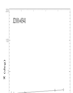
Figure 2: Examples of $\chi$ vs $\lambda^{2}$ fits discussed in the text. Upper panel: the fit to the source J2101+0341 as an example of a good linear interpolation. Middle panel: the fit to the source J0357+2319 as an example of a good interpolation with the addition of $n\pi$. Lower panel: the case of J2024+1718 whose RM cannot be fitted even with the addition of $n\pi$.

Table 5: Observed and Intrinsic Rotation Measures RM_obs and RM_int computed considering either high-frequency bands (from C to K; RM^h-f), or low-frequency bands (from L and C bands; RM^l-f); the Depolarization computed between C and X bands, and the intrinsic position angle $\chi_{\rm int}$. nf: data not fitted by a linear interpolation. When the redshift is unknown, we compute the RM_int assuming z=1.0.

Source	z	RM${}_{\rm obs}^{\rm h-f}$	RM${}_{\rm int}^{h-f}$	RM${}_{\rm obs}^{\rm l-f}$	RM${}_{\rm int}^{l-f}$	DP${}_{X}^{C}$	$\chi_{\rm int}$
		rad/m-2	rad/m-2	rad/m-2	rad/m-2		deg
J0217+0144	1.715	50	369	20	147	0.6	74
J0329+3510	0.5	388	873	12	27	1.7	17
J0357+2319		66	264	25	100	1.0	-86
J0519+0848		74	296	-39	-156	2.0	69
J0625+4440		-28	-112	5	20	1.1	-80
J0642+6758	3.18	-152	-2656	-	-	2.2	-46
J0646+4451	3.396	42	811	6	116	0.5	17
J1457+0749		22	88	-	-	1.1	-40
J1505+0326	0.411	2	6	43	86	0.2	-46
J1616+0459	3.197	202	3558	-	-	0.1	-97
J1645+6330	2.379	-129	-1473	-26	-297	0.4	75
J1811+1704		915	3660	-	-	0.8	-58
J2024+1718	1.05	nf		-	-	0.2
J2101+0341	1.013	47	190	-	-	0.9	-75
J2123+0535	1.878	373	3090	-13	-108	1.2	-6
J2212+2355	1.125	-177	799	19	86	0.8	40
J2320+0513	0.622	62	163	-5	-13	1.7	56
J2330+3348	1.809	365	2880	-10	-79	2.6	-92

4 Discussion and conclusions

Multi-frequency polarimetric measurements of a sample of young radio sources (Fanti et al. cf04 (2004); Cotton et al. cotton03 (2003)) show that very compact objects ($<$1 kpc) are unpolarized or strongly depolarized, and the fractional polarization is strictly related to the frequency: the lower the frequency, the stronger the depolarization.
On the other hand, blazars may not be intrinsically compact, but they are foreshortened because of projection effects (Antonucci anto93 (1993)). Since these objects are seen at small observing angles, their nuclear radio emission crosses a thinner slab of the magneto-ionic ambient medium and therefore Faraday rotation and depolarization are only marginally affected, contrary to what happens in radio sources with the axis oriented close to the plane of the sky. We find the same behaviour when we compare the fractional polarization of radio sources with different optical counterparts. HFPs associated with quasars and BL Lacs have higher polarization percentages than galaxies and empty fields, in agreement with unified schemes.
Several studies of the polarimetric properties in blazars have shown that these objects display a fractional polarization from $\sim 1\%$ up to $\sim$10%, almost constant at all frequencies (Klein et al. uk03 (2003); Saikia et al. saikia98 (1998)), and a polarization variability on different time-scales, from a few days to several years (Saikia & Salter ss88 (1988)), which can also be unrelated to the total intensity flux density variability. These objects usually have small rotation measures, becoming larger moving to higher frequency (e.g. Saikia et al. saikia98 (1998); O’Dea odea89 (1989)). Such a trend also has been found in our sources, rotation measures computed between L and C bands being much smaller than those between C and K bands. Furthermore, if we consider all the bands together (from L to K) no linear fit could interpolate the data. This may be explained assuming that the low and high frequency emissions originate from different regions of the radio jet.
In this scenario, the polarimetric properties are a key element for the determination of different classes of radio sources.
The information derived in this way becomes more effective if other selection tools, such as flux density variability (Paper I; Tinti et al. st05 (2005)) and morphological information (Orienti et al. mo06 (2006)) are taken into account.
From the analysis of our multi-frequency polarimetric data, we find that 12 sources ($\sim$26%) show polarized emission $>$1% at all the available frequencies, while another 17 objects ($\sim$38%) are completely unpolarized. In a sample of compact sources, such a percentage of highly-polarized objects reflects a strong contamination by blazar radio sources.
We find that 14 ($\sim 82\%$) of the unpolarized sources do not show any significant variability. On the other hand, all the highly-polarized ($m$ $>$1%) sources have strong flux-density variability and 11 ($\sim 65\%$) no longer show a convex spectrum.
If we analyze the polarized emission in relation to the pc-scale morphology (Orienti et al. mo06 (2006)), we find that HFPs with or without a CSO-like structure have different polarization properties: 12 ($\sim 86\%$) of the CSO-like sources are completely unpolarized at all frequencies, while 12 ($\sim 60\%$) of those without a CSO-like structure have highly-polarized ($m$ $>$ 1%) emission at each frequency.
All these pieces of evidence confirm the idea that the “bright” HFP sample (Dallacasa et al. dd00 (2000)) is made of two different radio source populations. If all the discriminant tools (variability, morphology, polarization) are considered together, we find that at least 33 ($\sim 60\%$) objects of the whole sample are contaminant objects, and only 22 ($\sim 40\%$) display all the typical characteristics of young radio source candidates. Furthermore, all the galaxies of the sample are still considered young radio sources, supporting the idea that the majority of galaxies and quasars represent two different radio source populations.

- (1) Alexander, P. 2000, MNRAS, 319, 8
- (2) Antonucci, R. ARA&A, 31, 473
- (3) Burn, B.F. 1966, MNRAS, 133, 67
- (4) Condon, J.J., Cotton, W.D., Greisen, E.W. et al. 1998, AJ, 115, 1693
- (5) Cotton, W.D., Dallacasa, D., Fanti, C. et al. 2003, PASA, 20, 12
- (6) Dallacasa, D., Stanghellini, C., Centonza, M., Fanti, R. 2000, A&A, 363, 887
- (7) Dallacasa, D. 2003, PASA, 20, 79
- (8) Fanti, C., Fanti, R., Dallacasa, D., Schilizzi, R.T. et al. 1995, A&A, 302, 317
- (9) Fanti, C., Branchesi, M., Cotton, W.D. et al. 2004, A&A, 427, 465
- (10) Klein, U., Mach, K.-H., Gregorini, L., Vigotti, M. 2003, A&A, 406, 579
- (11) Marecki, A., Spencer, R.E., Kunert, M. 2003, PASA, 20. 46
- (12) McCarthy, P.J. 1993, ARA&A, 31, 639
- (13) O’Dea, C.P. 1989, A&A, 210, 35
- (14) O’Dea, C.P., Baum, S.A. 1997, AJ, 113, 148
- (15) O’Dea, C.P. 1998, PASP, 110, 493
- (16) Orienti, M., Dallacasa, D., Tinti, S., Stanghellini. C. 2006, A&A, 450, 959
- (17) Orienti, M., Dallacasa, D., Stanghellini, C. 2007, A&A, in press, Paper I
- (18) Readhead, A.C.S., Taylor, G.B., Xu, W., Pearson, T.J. et al. 1996, ApJ, 460, 612
- (19) Rossetti, A., Fanti, C., Fanti, R., et al., submitted to A&A
- (20) Saikia, D.J., Salter, C.J. 1988, ARA&A, 26, 93
- (21) Saikia, D.J., Holmes, G.F., Kulkarni, A.R., Salter, C.J., Garrington, S.T. 1998, MNRAS, 298, 877
- (22) Saikia, D.J. 1999, MNRAS, 302, 60L
- (23) Snellen, I.A.G., Schilizzi, R.T., Miley, G.K. et al. 2000, MNRAS, 319, 445
- (24) Stanghellini. C., O’Dea, C.P., Dallacasa, D., et al. 1998, A&AS, 131, 303
- (25) Stanghellini, C., O’Dea, C.P., Dallacasa, D. et al. 2005, A&A, 443, 891
- (26) Tinti, S., Dallacasa, D., de Zotti, G., Celotti, A., Stanghellini, C. 2005, A&A, 432,31
- (27) Urry, M.C., Padovani, P. 1995, PASP, 107, 803
- (28) Wilkinson, P.N., Polatidis, A.G., Readhead, A.C.S., Xu, W., Pearson, T.J. 1994, ApJ, 432, 87