Event-Driven Dynamics of Rigid Bodies Interacting via Discretized Potentials

Abstract

A framework for performing event-driven, adaptive time step simulations of systems of rigid bodies interacting under stepped or terraced potentials in which the potential energy is only allowed to have discrete values is outlined. The scheme is based on a discretization of an underlying continuous potential that effectively determines the times at which interaction energies change. As in most event-driven approaches, the method consists of specifying a means of computing the free motion, evaluating the times at which interactions occur, and determining the consequences of interactions on subsequent motion for the terraced-potential. The latter two aspects are shown to be simply expressible in terms of the underlying smooth potential. Within this context, algorithms for computing the times of interaction events and carrying out efficient event-driven simulations are discussed. The method is illustrated on system composed of rigid rods in which the constituents interact via a terraced potential that depends on the relative orientations of the rods.

I Introduction

Simulating systems with discontinuous interactions offers a number of advantages over standard molecular dynamics simulations (SMD) in which the solution of a system of ordinary differential equations is solved numerically by iterating a map which approximates the short-time dynamicsFrenkelSmit . The advantage of simulating discontinuous systems using event-driven algorithmsRapaport80 (discontinuous molecular dynamics, or DMD) over SMD is particularly apparent for systems of low density, where the short-time mapping of the dynamics in SMD is applied to freely evolve the majority of the system. In spite of the rarity of interactions at low density, the inherent time step in SMD simulations cannot be increased beyond some small threshold without loss of stability and accuracy of trajectories, since there is nearly always a small fraction of particles interacting at any given time. Several adaptive integration methods exist, typically based on either separating rapidly and slowly-varying components of the potential in a multiple time step approachmts , or on time re-parametrization of the Hamiltonian equations to a new system that is integrated with a fixed step sizereparam . Both methods have inherent drawbacks making them unsuitable for arbitrary potentials. On the other hand, in the event-driven approach where there is no inherent time step, each non-interacting particle is not propagated forward in time until it interacts with another particle in the system.

Event driven simulations also have some rather serious drawbacks. For example, simulations of flexible molecular systems are plagued with processing often irrelevant intra-molecular events on very rapid time scales, wasting a great deal of computation. When physically reasonable, much can be gained by treating the molecules as rigid. Although the general framework for performing event-driven simulations of rigid or constrained systems has been recently worked outdmdMethod , numerical methods must be used to find interaction times, potentially leading to gross inefficiencies. Another clear drawback that discourages the use of the DMD approach is that little is known about how to design site-based, stepped interaction potentials between such rigid bodies, and much work must be done to tune interaction parameters, such as well-depths and interaction distances at which discontinuities occur. The design of a distance-based, discontinuous potential for long-ranged electrostatic interactions seems particularly problematic.

In this article, possible solutions for both these problems in DMD simulations are presented. An algorithm based upon an adaptive grid search is presented as an alternative to the uniform grid approach of Ref. dmdMethod, to make the search for interaction times as efficient as possible. We also demonstrate here how the issue of designing detailed discontinuous potentials can be side-stepped altogether by using a mapping of an underlying continuous pair potential onto discrete potential energy values. The potential energy then consists of a set of allowed energy terraces, each mapped onto by many different positions and orientations of the system. The discretization of the potential energy on the level of the pair potential implies that the evolution consists of free propagation of the system punctuated by impulses at discrete times when the underlying continuous interaction potential for a pair of particles hits a critical value. Because the scheme uses ordinary continuous interaction potentials as its basis, no substantial effort is required to parameterize the Hamiltonian, and the experience of many years of work in the modeling of systems can be exploited. The method is applicable to any type of pair-interaction potential, and can be used with potentials written for rigid systems that depend on the center of mass positions as well as the relative orientation of two interacting bodiesgayBerne ; fastWater .

The paper is organized as follows: Sec. II reviews the elements of rigid body mechanics required to formulate the method. In Sec. III, a general description to numerically find interaction times is presented. A derivation of the consequences of the action of the impulsive forces and torques on the system is given in Sec. IV. The scheme is applied to a simple model system with orientationally-dependent interactions in Sec. V. Final comments are given in Sec. VI.

II Rigid Systems Interacting Via Stepped-Potentials

The systems considered here consist of $N$ rigid bodies, each of mass $m$ and moment of inertia tensor $\mathsf{I}_{i}$. Associated with each object $i$ are a center of mass position and velocity $\mathbf{r}_{i}$ and $\mathbf{v}_{i}$, an attitude or orientation matrix $\mathsf{A}_{i}$, and an angular velocity vector $\bm{\omega}_{i}$. The attitude matrix $\mathsf{A}_{i}$ transforms a vector $\mathbf{a}$ with respect to a fixed inertial lab reference frame to its representation $\tilde{\mathbf{a}}=\mathsf{A}_{i}\mathbf{a}$ in the principal-axis frame of body $i$. $\mathsf{A}_{i}$ is in fact defined such that the moment of inertia tensor is diagonal in the principal axis frame: $\tilde{\mathsf{I}}_{i}=\mathsf{A}^{\dagger}_{i}\mathsf{I}_{i}\mathsf{A}_{i}=\mathrm{diag}(I_{i1},I_{i2},I_{i3})$, where $I_{i1}$, $I_{i2}$ and $I_{i3}$ are the (possibly distinct) principal moments of inertia of body $i$. Although there are several ways to parametrize the attitude matrix $\mathsf{A}$, such as Euler angles, unit quaternions, or angle-axisGoldstein coordinates, three generalized coordinates are always required to specify the orientation of each three-dimensional rigid body, denoted here by $\bm{\vartheta}_{i}=(\vartheta_{i1},\vartheta_{i2},\vartheta_{i3})$. The time derivative of $\bm{\vartheta}_{i}$ can be related to $\bm{\omega}_{i}$ by noting that $\bm{\omega}_{i}$ is related to the time derivative of the attitude matrix viaVanZonSchofieldCompPhys

$$\sum_{a=x,y,z}\varepsilon_{bac}(\bm{\omega}_{i})_{a}=\sum_{a=x,y,z}(\dot{\mathsf{A}}_{i})_{ab}(\mathsf{A}_{i})_{ac},$$ (1)

where $\varepsilon_{bac}$ is the Levi-Civita symbol.Goldstein From this relation, one can easily derive that $\bm{\omega}_{i}=\mathsf{N}_{i}^{\dagger}\dot{\bm{\vartheta}}_{i}$, where $(\mathsf{N}_{i})_{ab}=\frac{1}{2}\varepsilon_{bcd}(\mathsf{A}_{i})_{ec}\partial(\mathsf{A}_{i})_{ed}/\partial(\bm{\vartheta}_{i})_{a}$.

If the system is governed by a smooth potential $U$, then the equations of motion imply that

$$\dot{\mathbf{p}}_{i} =-\frac{\partial U}{\partial\mathbf{r}_{i}}=\mathbf{F}_{i}; \dot{\mathbf{L}}_{i} =-\mathsf{N}^{-1}_{i}\frac{\partial U}{\partial\bm{\vartheta}_{i}}\equiv\bm{\tau}_{i},$$ (2)

where $\mathbf{p}_{i}=m\mathbf{v}_{i}$ is the (linear) momentum of body $i$, $\mathbf{L}_{i}=\mathsf{I}_{i}\bm{\omega}_{i}$ is the angular momentum of that body with respect to its center of mass, $\mathbf{F}_{i}$ is the force on the center of mass of body $i$, and $\bm{\tau}_{i}$ is the torque on body $i$.

In many cases, the formal expression for the torque in Eq. (2) can be written in compact form which does not depend on the choice of parametrization of the attitude matrix $\mathsf{A}_{i}$. For example, if the potential can be written in terms of site-site interactions, the center of mass force $\mathbf{F}_{i}=\sum_{\gamma}\mathbf{F}_{i\gamma}$ is a sum of the forces $\mathbf{F}_{i\gamma}$ acting on the sites $\gamma$, and the torque can be written as

$$\bm{\tau}_{i} =\sum_{\gamma}\left(\mathbf{r}_{i\gamma}-\mathbf{r}_{i}\right)\times\mathbf{F}_{i\gamma},$$ (3)

where $\mathbf{r}_{i\gamma}$ is the position of site $\gamma$ on body $i$.

A second example where one can write simple expressions for $\mathbf{F}_{i}$ and $\bm{\tau}_{i}$ is if the potential $U$ is a sum of pair potentials $U_{ij}$ between bodies $i$ and $j$, each of which is rotationally invariant but depends on inner products of the relative position vector $\mathbf{r}_{ij}=\mathbf{r}_{i}-\mathbf{r}_{j}$ and a set of orientationally dependent vectors $\mathbf{s}_{i}^{\alpha}$ and $\mathbf{s}_{j}^{\beta}$ (where $\alpha$ and $\beta$ are integers indicating different vectors for body $i$ and $j$, respectively). Then the force and torque on body $i$ due to interactions with body $j$ through the interaction potential $U_{ij}(\mathbf{r}_{ij},\{\mathbf{s}_{i}^{\alpha}\},\{\mathbf{s}_{j}^{\beta}\})$ can be written as

$$\mathbf{F}_{ij} =-\frac{\partial U_{ij}}{\partial r_{ij}}\hat{\mathbf{r}}_{ij}-\sum_{\alpha}\frac{\partial U_{ij}}{\partial(\mathbf{r}_{ij}\cdot\mathbf{s}_{i}^{\alpha})}\mathbf{s}_{i}^{\alpha}-\sum_{\beta}\frac{\partial U_{ij}}{\partial(\mathbf{r}_{ij}\cdot\mathbf{s}_{j}^{\beta})}\mathbf{s}_{j}^{\beta}$$ (4)

$$\bm{\tau}_{ij} =-\sum_{\alpha,\beta}\frac{\partial U_{ij}}{\partial(\mathbf{s}_{i}^{\alpha}\cdot\mathbf{s}_{j}^{\beta})}\,\mathbf{s}_{i}^{\alpha}\times\mathbf{s}_{j}^{\beta}-\sum_{\alpha}\frac{\partial U_{ij}}{\partial(\mathbf{r}_{ij}\cdot\mathbf{s}_{i}^{\alpha})}\,\mathbf{s}_{i}^{\alpha}\times\mathbf{r}_{ij}$$ (5)

where we have used Eq. (2) and the fact that $\varepsilon_{bde}(\mathsf{N}_{i})_{ab}=(\mathsf{A}_{i})_{cd}\,\partial(\mathsf{A}_{i})_{ce}/\partial(\bm{\vartheta}_{i})_{a}$. Using the expressions of the forces in Eq. (4), one finds for each interacting pair $\mathbf{F}_{ij}+\mathbf{F}_{ji}=0$, which implies conservation of total linear momentum $\sum_{i}\mathbf{p}_{i}$. Furthermore, using the torques in Eq. (5), it is straightforward to verify that

$$\mathbf{r}_{i}\times\mathbf{F}_{ij}+\mathbf{r}_{j}\times\mathbf{F}_{ji}+\bm{\tau}_{ij}+\bm{\tau}_{ji}=0,$$ (6)

which, in turn, implies that the total angular momentum $\sum_{i}(\mathbf{L}_{i}+\mathbf{r}_{i}\times\mathbf{p}_{i})$ is conserved by the dynamics.fna

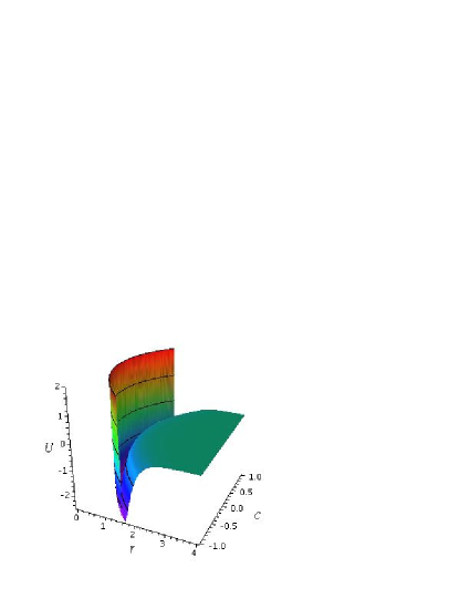
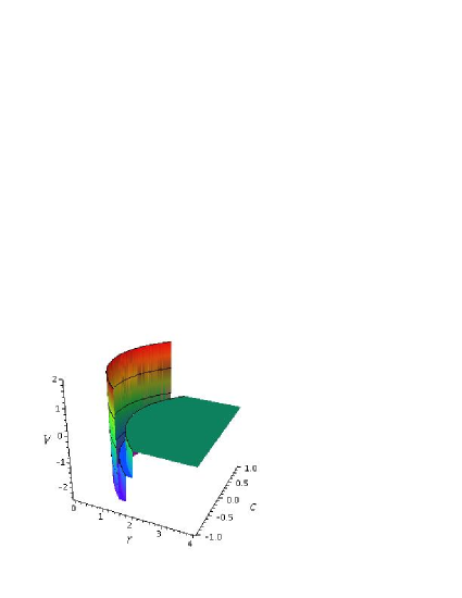
Figure 1: Illustration of the potential energy discretization procedure given in Eq. (7) applied to the potential in Eq. (22) of Sec. V, with the $\epsilon=5/2$, $\sigma=1$ and $\Delta=1$. The top panel shows the continuous potential $U$ and the bottom panel the terraced variant $V$ if $V_{min}=-2$, $\Delta V_{k}=\Delta V=1$ and $U_{k}=V_{min}+(k-\frac{1}{2})\Delta V$. On the axes, $r=|\mathbf{r}_{i}-\mathbf{r}_{j}|$ and $c=\mathbf{s}_{i}\cdot\mathbf{s}_{j}$.

So far we have considered $U$ to be a continuous potential, which is required for the derivatives in the above equations to exist. Now we consider a stepped interaction potential between a pair $i$, $j$ of bodies bases on a continuous potential $U_{ij}$, such that the interaction potential between bodies $i$ and $j$ is of the form

$$V_{ij} =V_{min}+\sum_{k=1}^{K}\Theta(U_{ij}-U_{k})\Delta V_{k},$$ (7)

where $\Theta(x)$ is the Heaviside function, and $U_{k}$ are a discrete sets of values of the smooth potential at which the system gains or loses potential energy $\Delta V_{k}$. Note that for a system in which the underlying continuous interaction energy $U_{ij}$ between bodies $i$ and $j$ lies anywhere in the range $U_{k}<U_{ij}<U_{k+1}$, the form of Eq. (7) assigns a constant potential energy value of $V_{min}+\sum_{k^{\prime}=1}^{k}\Delta V_{k^{\prime}}$ to this interaction. Figure 1 contains an illustration of the result of this procedure for the potential energy function given in Eq. (22). Because of the shape of the potential energy landscape, we call a potential of the form (7) a terraced potential.

For a system in which all interactions are of terraced form, the procedure to evaluate dynamical properties is the same as that in simulations of hard sphere systemsdmdMethod . While the system has constant potential energy between interaction events, the motion of the system is free and the trajectory of each constituent is independent of all others. The free propagation of the system between events determines the evolution of the spatial coordinates of the molecules in the system, and the interaction times at which the momenta of the system change discontinuously is determined by identifying the times at which the underlying continuous pair potential energy $U_{ij}$ hits an energy terrace $U_{k}$ where the potential energy changes discontinuously. Even though this interaction time is determined by free motion of the system, in general, it must be found numerically due to the mathematical complexity of the interaction condition. The next section addresses this problem. The final ingredient required to perform event-driven simulations of systems consists of specifying the interaction rules of how the momenta of the constituents in the molecular system are altered at the interaction times and is worked out in Sec. IV.

III Finding Interaction Event Times

For systems with terraced potentials as in Eq. (7), the particles evolve freely until a configuration of the system is reached where the instantaneous value of the underlying continuous potential $U_{ij}$ equals $U_{k}$, for some pair of particles $i$ and $j$. The first time at which such an event occurs can be solved by finding the smallest positive zero (root) of the indicator equation

$$f_{ij}(t) =U_{ij}\bigl{(}\mathbf{r}_{ij}(t),\{\mathbf{s}^{\alpha}_{i}(t)\},\{\mathbf{s}^{\beta}_{j}(t)\}\bigr{)}-U_{k},$$ (8)

where the time dependence of the indicator function $f_{ij}$ is determined by the free trajectories of bodies $i$ and $j$. Although the time dependence of the relative vector $\mathbf{r}_{ij}(t)=\mathbf{r}_{ij}(0)+(\mathbf{v}_{i}-\mathbf{v}_{j})t$ appearing in the indicator function is simple in the case of free motion, the time-dependence of the orientational vectors $\mathbf{s}_{i}^{\alpha}(t)$ and $\mathbf{s}_{j}^{\beta}(t)$ depends on the evolution of the attitude matrices $\mathsf{A}_{i}(t)$ and $\mathsf{A}_{j}(t)$, since these vectors may be expressed as

$$\mathbf{s}_{i}^{\alpha}(t) =\mathsf{A}^{\dagger}_{i}(t)\,\tilde{\mathbf{s}}_{i}^{\alpha}$$ (9)

$$\mathbf{s}_{j}^{\beta}(t) =\mathsf{A}^{\dagger}_{j}(t)\,\tilde{\mathbf{s}}_{j}^{\beta},$$ (10)

where $\tilde{\mathbf{s}}_{i}^{\alpha}$ and $\tilde{\mathbf{s}}_{j}^{\beta}$ are time-independent vectors in the body frames of particles $i$ and $j$, respectively.

The form of the time dependence of the attitude matrices $\mathsf{A}_{i}(t)$ depends on the way in which mass is distributed in the rigid bodies. Nonetheless, it is possible to write down analytical expressions for the time-dependence of $\mathsf{A}_{i}$ even when the mass of a body is not symmetrically distributed. The general solution of $\mathsf{A}_{i}(t)$ can always be written in the formVanZonSchofieldCompPhys

$$\mathsf{A}_{i}(t) =\mathsf{P}_{i}(t)\cdot\mathsf{A}_{i}(0),$$ (11)

where the matrix $\mathsf{P}_{i}(t)$ propagates the orientation matrix from an initial time to time $t$. The precise forms of $\mathsf{P}_{i}(t)$ for different kinds of rotor can be found in Ref. VanZonSchofieldCompPhys, .

Even with analytical expressions for the time-dependence of the underlying potential $U_{ij}(t)$, the earliest interaction time must be found numerically, as was also the case for event-driven dynamics for rigid systems interacting via site-site potentialsdmdApplication . However, one major benefit of utilizing an energy terracing approach is that there is only a single one-dimensional root search to be conducted for each pair of interacting bodies, in contrast to a site-based energy approach in which all pairs of sites between pairs of molecules must be examined for the earliest interaction time.

In Ref. dmdMethod, , a simple approach to find the earliest interaction time was given in which screening methods are used to identify a minimum and maximum time between which a root of the indicator function could lie. This interval is then sub-divided into equally-sized smaller intervals of fixed size $\Delta t$ and used to bracket sign changes of the indicator function. Unfortunately, for translating and rotating rigid bodies, the indicator function is oscillatory, making the detection of so-called grazing interactions troublesome unless a very small grid interval $\Delta t$ is used. Since the indicator function has a local extremum in a grazing interaction, a good strategy to find this kind of event is to determine the minimum or maximum of the indicator function in cases in which the indicator function $f_{ij}(t)$ itself does not change sign, but its derivative $\dot{f}_{ij}(t)$ does. However, in the vicinity of a grazing interaction, the values of the indicator function are typically small, and hence only extrema where the indicator function at one of the grid points lies below some threshold value need to be investigated. Efficient numerical routines exist to find local extrema of a one-dimensional functionNumRecipes ; Brent , and thereby detect grazing interactions. Once an interval with a change in sign of the indicator function has been identified, standard techniques can be invoked to find the rootNumRecipes ; Brent .

Although the scheme outlined above is fairly robust and can detect many millions of events without missing roots, its efficiency is strongly dependent on the choice of basic time interval $\Delta t$. In many cases, the size of this interval is determined not by the typical rate of change of the indicator function but by certain rare scenarios where rapid changes in the indicator function and its derivative and multiple local extrema occur. Unnecessarily small time intervals can be avoided by using the following adaptive bracketing scheme based on cubic interpolation to estimate the indicator function and the number of extrema in a given interval.

The basic idea is to use information from previous grid points as much as possible. Note that when evaluating the indicator function $f$ at a certain point $t$, it is very easy to also compute its time derivative. For a given pair of molecules $i$ and $j$ and assuming a terraced-interaction potential based on the continuous pair potential $U_{ij}(\mathbf{r}_{ij},\left\{\mathbf{s}_{i}\right\},\left\{\mathbf{s}_{j}\right\})$, the time derivative of the indicator function $f_{ij}(t)$ is given by

$$\dot{f}_{ij}(t) =-\mathbf{F}_{ij}\cdot\mathbf{v}_{ij}-\bm{\tau}_{ij}\cdot\bm{\omega}_{i}-\bm{\tau}_{ji}\cdot\bm{\omega}_{j},$$ (12)

where $\mathbf{v}_{ij}=\mathbf{v}_{i}-\mathbf{v}_{j}$ is the relative velocity vector for the centers of mass, $\mathbf{F}_{ij}$ is the force on $i$ due to $j$, and $\bm{\tau}_{ij}$ and $\bm{\tau}_{ji}$ are the torques on $i$ and $j$, as given by the smooth interaction in Eqs. (4) and (2).

At the start of the search for the first root of the function $f_{ij}$, its value and derivative are computed. A linear extrapolation $f_{\ell}(t)=f_{1}+\dot{f}_{1}\,t$ can be used to get an estimate $t^{\prime}$ for the root of $f_{ij}$ by solving $f_{\ell}(t^{\prime})=0$. The next grid point is then taken to be $t_{2}=t^{\prime}+\delta t$, where a small $\delta t$ is added to enhance the probability of a sign change of $f_{ij}$ in $[0,t_{2}]$. At $t=t_{2}$, the function and its derivative are evaluated. If there is a sign change in $f_{ij}$, a root has been bracketed and a numerical root search using standard techniques is usedNumRecipes ; Brent . Otherwise, given the value of the indicator function and its derivative at two times, a unique cubic interpolation of the indicator function can be constructed. For example, consider the indicator function $f(t)$ satisfying $f(0)=f_{1}$, $f(\Delta t)=f_{2}$ with time derivatives $\dot{f}(0)=\dot{f}_{1}$ and $\dot{f}(\Delta t)=\dot{f}_{2}$. Using these values, the cubic approximation $f_{c}(t)$ for the indicator function over the interval is

$$f_{c}(t) =f_{1}+\dot{f}_{1}\,t+\alpha\,t^{2}+\beta\,t^{3},$$ (13)

where

$$\alpha =\frac{3(f_{2}-f_{1})-(2\dot{f}_{1}+\dot{f}_{2})\Delta t}{\Delta t^{2}}$$ (14)

$$\beta =\frac{2(f_{1}-f_{2})+(\dot{f}_{1}+\dot{f}_{2})\Delta t}{\Delta t^{3}}.$$ (15)

The number of extrema in the interval $[0,\Delta t]$ is then estimated by finding the number of real roots of the equation $\dot{f}_{c}(t)=0$ in the interval. Furthermore, the values of the extrema are easily obtained using (13).

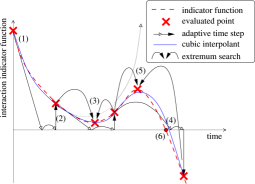
Figure 2: Example of the adaptive root search with cubic interpolation.

The adaptive procedure using the cubic approximants is most-easily explained by considering the example in Fig. 2. Consider beginning the process of looking for a root after an interaction event. In this scenario, at point $(1)$ in the figure, only the value of the indicator function and its derivative are known at $t=0$. The next bracketing point is chosen by solving $f_{\ell}(t^{\prime}_{2})=0$. If the time $t^{\prime}_{2}$ is very large or infinite, the next bracketing time $t_{2}$ is chosen to be some default (and regular) value, $\Delta t$. On the other hand if $t^{\prime}_{2}<\Delta t$, the second bracketing time $t_{2}=t^{\prime}_{2}+\delta t$ is chosen. At point $(2)$, the indicator function and its derivative are evaluated and the cubic and linear approximations to the function evaluated. The linear and cubic equations are then examined for roots. In the case shown in Fig. 2, the cubic approximation has no roots whereas the linear interpolant does, at $t^{\prime}_{3}$. Since $t^{\prime}_{3}<t_{2}+\Delta t$, the next bracketing point is selected to be $t_{3}=t^{\prime}_{3}+\delta t$. But the cubic interpolant has a local minimum in the interval $[t_{2},t_{3}]$, so a minimum search algorithm is used to find the actual minimum of $f_{ij}$ at (3). Since $f_{ij}$ is found to be positive at (3), a potential grazing interaction has been ruled out. The root of the cubic $t^{\prime}_{4}$ is then used to place the next bracketing point at $t_{4}=t_{4}+\delta t$. The cubic interpolant using points $t_{3}$ and $t_{4}$ reveals that there is a local maximum in this interval, and that there is a sign change in the indicator function in the interval since $f(t_{4})<0$. The local maximum is investigated and found to be positive at time $t_{5}$, so the final bracketing interval where a root is found is taken to be $[t_{5},t_{4}]$, leading to the root at point $(6)$.

IV Interaction rules

If the total interaction potential for the system is a pairwise-additive combination of terraced two-body interaction potentials of the form (7), then forces and torques only act instantaneously on a pair of molecules $i$ and $j$ at a time determined by when $U_{ij}$ is equal to one of the reference values $U_{k}$. The forces and torques are therefore impulsive, and lead to discontinuous changes in the linear and angular momenta of the pair. The effect of the impulses must be consistent with conservation conditions that arise from the symmetries of the overall Hamiltonian, such as the conservation of energy, and conservation of total linear and total angular momenta.

Since the momenta and angular momenta change discontinuously and are not well-defined at an interaction time $t_{c}$, a more practical starting point for deriving the interaction rules is to consider the effect of impulses applied to the overall change in the momentum and angular momentum of interacting bodies $i$ and $j$ over a small time interval $[t_{c}-\delta,t_{c}+\delta]$:

$$\mathbf{p}_{i}^{\prime} =\mathbf{p}_{i}+\int_{t_{c}-\delta}^{t_{c}+\delta}\mathbf{F}_{i}(t)dt$$ (16)

$$\mathbf{L}_{i}^{\prime} =\mathbf{L}_{i}+\int_{t_{c}-\delta}^{t_{c}+\delta}\bm{\tau}_{i}(t)dt,$$ (17)

with analogous expressions for molecule $j$. In Eqs. (16) and (17), the primed and unprimed vectors represent post and pre-interaction values of the respective quantities. For small enough $\delta$, the probability of a particle other than $j$ interacting with $i$ becomes zero. From Hamilton’s equations for the discontinuous system, the impulsive forces and torques are then given by

$$\mathbf{F}_{i}(t) =S^{f}_{i}\mathbf{F}_{ij}(t_{c})\delta(t-t_{c})$$ (18)

$$\bm{\tau}_{i}(t) =S^{l}_{i}\bm{\tau}_{ij}(t_{c})\delta(t-t_{c}),$$ (19)

where $\mathbf{F}_{ij}(t_{c})$ and $\bm{\tau}_{ij}(t_{c})$ are the forces and torques on body $i$ at the interaction time $t_{c}$ for the continuous system given in Eqs. (4) and (5), and $S^{f}_{i}$ and $S^{l}_{i}$ are unknown scalars. Note that the directions of the impulsive forces and torques due to the pair interaction are along the directions of those quantities for a continuous system interacting by the same potential at the interaction time. For the interaction pair $i$-$j$, conservation of linear momentum immediately implies that $S^{f}_{j}=S^{f}_{i}=S^{f}$. The requirement of conservation of total angular momentum furthermore gives

$$(S_{i}^{l}-S_{j}^{l})\sum_{\alpha,\beta}\frac{\partial U_{ij}}{\partial(\mathbf{s}_{i}^{\alpha}\cdot\mathbf{s}_{j}^{\beta})}(\mathbf{s}_{i}^{\alpha}\times\mathbf{s}_{j}^{\beta})\\ +(S_{i}^{l}-S^{f})\sum_{\alpha}\frac{\partial U_{ij}}{\partial(\mathbf{s}_{i}^{\alpha}\cdot\mathbf{r}_{ij})}(\mathbf{s}_{i}^{\alpha}\times\bm{r}_{ij})\\ +(S_{j}^{l}-S^{f})\sum_{\beta}\frac{\partial U_{ij}}{\partial(\mathbf{s}_{j}^{\beta}\cdot\mathbf{r}_{ij})}(\mathbf{s}_{j}^{\beta}\times\bm{r}_{ij})=0.$$ (20)

Since this condition must be satisfied for arbitrary vectors $\mathbf{r}_{ij}$, $\mathbf{s}_{i}^{\alpha}$, $\mathbf{s}_{j}^{\beta}$, we conclude that $S_{i}^{l}=S_{j}^{l}=S^{f}=S$.fnb The unknown scalar $S$ is now found from conservation of energy, by solving the quadratic equation

$$\biggl{(}\frac{\mathbf{F}_{i}\cdot\mathbf{F}_{i}}{m}+\frac{\bm{\tau}_{i}\cdot\mathsf{I}_{i}^{-1}\cdot\bm{\tau}_{i}}{2}+\frac{\bm{\tau}_{j}\cdot\mathsf{I}_{j}^{-1}\cdot\bm{\tau}_{j}}{2}\biggr{)}S^{2}\\ +(\mathbf{v}_{ij}\cdot\mathbf{F}_{i}+\bm{\tau}_{i}\cdot\bm{\omega}_{i}+\bm{\tau}_{j}\cdot\bm{\omega}_{j})S+\Delta V=0,$$ (21)

where all quantities are evaluated at interaction time $t_{c}$ and $\Delta V$ is the change in potential energy. Note that the term proportional to $S$ can also be written as $-\dot{U}_{ij}(t_{c})$, as follows from Eq. (12). The physical solution corresponds to the positive (negative) root branch if $\dot{U}_{ij}(t_{c})<0$ ($\dot{U}_{ij}(t_{c})>0$), provided real roots exist. If this latter condition is not met, there is not enough kinetic energy to overcome the discontinuous barrier, and the system experiences a reflection with no change in potential energy, i.e., $S$ is the non-zero solution of Eq. (21) with $\Delta V=0$.

V Model System

As an illustration of the method, consider a system composed of rods in which the continuous interaction potential between a given pair $i$-$j$ is of a modified Lennard-Jones form

$$U_{ij} =4\epsilon\left[\left(\frac{\sigma}{r_{e}}\right)^{12}-\left(\frac{\sigma}{r_{e}}\right)^{6}\right]$$ (22)

with

$$r_{e} =|\mathbf{r}_{ij}|+\zeta\left[\frac{1}{2}-(\mathbf{s}_{i}\cdot\mathbf{s}_{j})^{2}\right].$$ (23)

Here, $\mathbf{s}_{i}$ is a vector pointing along the long axis of the rod and $r_{e}$ defines an orientation dependent effective distance of interaction. Note that the form of this potential makes it energetically favorable to align adjacent rods orthogonal to one another.

By construction, the potential is invariant under rotations and translations and therefore the dynamics conserves the total linear and angular momentum in addition to the total energy of the system. Using Eqs. (2), (4) and (5), the force and torque on body $i$ due to interactions with $j$ is

$$\mathbf{F}_{ij} =-\frac{dU_{ij}}{dr_{e}}\hat{\mathbf{r}}_{ij}$$

$$\bm{\tau}_{ij} =2\zeta(\mathbf{s}_{i}\cdot\mathbf{s}_{j})\frac{dU_{ij}}{dr_{e}}\,\mathbf{s}_{i}\times\mathbf{s}_{j}$$

$$\frac{dU_{ij}}{dr_{e}} =-\frac{24\epsilon}{r_{e}}\left[2\left(\frac{\sigma}{r_{e}}\right)^{12}-\left(\frac{\sigma}{r_{e}}\right)^{6}\right].$$ (24)

Note that the torque on $i$ is orthogonal to the vector $\mathbf{s}_{i}$, so that the component of the angular momentum along the axis of the molecule is constant. Thus, even though the rotational dynamics of the rigid rods is that of a symmetric top, the angular motion around the long axis is decoupled from the other directions and can be neglected.

From this continuous system one can construct a system with a terraced potential. In the current study, the simplest form of the terracing procedure will be used, where the discontinuities in the potential are evenly-spaced values of the interaction energy, i.e. in Eq. (7) all $\Delta V_{k}$ are taken to be equal and the values of $U_{k}$ are taken to be $U_{k}=(k-\frac{1}{2})\Delta V$. In practice, it is desirable to map a value of $U_{ij}\approx 0$ to zero, so that pairs that are far apart do not contribute potential energy to the system. This is readily accomplished by adjusting the value of $V_{min}$ in Eq. (7). It is also important that the critical values $U_{k}$ not coincide with minima of the smooth pair potential, because a terrace of width zero would result, leading to numerical instabilities.

It is interesting to consider how the graininess of the energy terraces influences dynamical phenomena, particular in dense systems where orientational relaxation times become quite long. To examine the sensitivity of dynamical correlations to the form of the stepped-potential, event-driven simulations of a system of $N=512$ rods at a reduced number density $\rho^{*}=\rho\sigma^{3}=0.5$ and reduced temperature $T^{*}=kT/\epsilon=1.4$ were carried out in a periodic, cubic box and contrasted with SMD simulations using the continuous underlying potential, Eq. (22). The parameters chosen for the system and pair potential were $\epsilon=3.0$ kJ/mol, $\sigma=3.035$ Å, $\zeta=1$ Å, $m=18$ g/mol, and $I_{1}=I_{2}=1.154$ g/mol-Ų.

V.1 Implementation of the event-driven simulation

As was observed in the case of event-driven simulations based on site-site potentialsdmdApplication , the efficiency of the event-driven approach can be greatly enhanced by implementing several simple and now fairly standard techniques, such as cell divisions, tree data structures to manage events, and local molecular clocksRapaport80 . In Ref. dmdMethod, , two additional techniques for improving the performance of event-driven simulations utilizing numerical methods of finding event times were also presented: the use of screening methods to identify initial and final bracket times, and the truncation of potentially non-useful event searches through the scheduling of a virtual interaction. To identify which pairs of particles could have interactions under the terracing potential for a given choice for the set of discontinuities, the maximum distance $r_{m}$ at which $U$ is larger than $\Delta V/2$ was found by solving the equation $U_{ij}=-\Delta V/2$ with $r_{e}=r_{m}-\zeta/2$, giving

$$r_{m}=\frac{1}{2}\zeta+\frac{\sigma}{\sqrt[6]{\frac{1}{2}[1-\sqrt{1-\Delta V/(2\epsilon)}]}}.$$ (25)

The system is then partitioned using this maximum interaction distance to determine the cell size so that only particles in the same or adjacent cells interact. For each pair of possibly interacting particles $i$ and $j$, the times at which the distance between center of masses reaches $r_{m}$ is solved exactly using the linear free motion of the pair to determine minimum and maximum bracketing times.

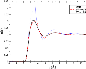
Figure 3: The radial distribution function for the center of mass of the rods.

To implement the virtual interaction event, a root search procedure for a given pair of rods was only conducted up to a maximum of $4$ femtoseconds before the root search was truncated, and if no root was found, the value of the indicator function and its derivative at the end point of the interval were stored in the tree to resume the search for the pair if neither particle has an event before the point at which the search was halted. A maximum step size of $\Delta t=4$ femtoseconds was also utilized in the adaptive search algorithm outlined in Sec. III.

The use of a uniform maximum step size generally leads to sub-optimal tree structures in the priority queue, where long linear branches corresponding to scheduled simultaneous virtual interaction events lead to longer insertion times of new events into the queue. Two countermeasures were employed to improve the management of the event queue: First, the maximum step size $\Delta t$ was given a small random adjustment to avoid the coincidence of any two virtual interactions. The effect of this adjustment is to form more balanced binary trees free of long linear branches. Second, a bounded priority queuePaul07 was used in which arrays of linear lists of events in a given time interval are combined with an implicit heap binary tree that performs a fine sort of the list containing the current time interval. The use of the linear lists enables rapid insertion of future events into the priority queue, and typically reduced the overall computational time by around $15\%$ for the system sizes investigated. It is expected that the advantage of the bounded priority queue over standard binary tree data structures will increase with increasing system size, since operations on the queue take $O(1)$ time per event, as opposed to $O(\log N)$ time.

To keep the tree structure from growing too large in the course of a simulation, standard scheduling schemes require canceling each event which becomes invalid due to the occurrence of an earlier interaction involving one of its participants. Tracking down these events in the tree requires a fair amount of bookkeepingRapaport80 . Directly canceling invalidated events could be done with the bounded priority queue as well, but there is no real need to do so since the tree component of the event queue is small already. Not removing invalid events from the queues was found to lead to another 15% reduction in computational time. The problem of growing linear lists was handled by a (relatively fast and infrequent) cleanup of invalid events from the lists when computer memory threatens to be depleted.

V.2 Comparison between standard molecular dynamics and event-driven simulations

To assess the relative merits of the DMD approach as opposed to a standard rigid body molecular dynamics approach, SMD simulation were carried out based on the pair potential in Eq. (22). The equations of motion were integrated using a symplectic integration scheme that utilizes the exact free motion for both rotational and translational degrees of freedomintegratorPapers . The time step used in the SMD simulations was $1.8$ femtoseconds, resulting in relative fluctuations of the total energy to the potential energy of about 1%. To improve the efficiency of the SMD simulations, Verlet lists were used.FrenkelSmit In addition, the potential was smoothly interpolated to zero starting from a cut-off distance of $r_{l}=2.5\sigma$ and reaching zero at a distance of $r_{u}=3\sigma$, by taking as the interaction potential

$$U_{ij}^{\rm{smooth}} =g(r_{ij})U_{ij}(\mathbf{r}_{ij},\mathbf{s}_{i},\mathbf{s}_{j})$$ (26)

where

$$g(r) =\left\{\begin{array}[]{ll}1&r<r_{l}\\ \frac{(r_{u}-r)^{2}(r_{u}-3r_{l}+2r)}{(r_{u}-r_{l})^{3}}&r_{l}\leq r\leq r_{u}\\ 0&r>r_{u}\end{array}\right..$$ (30)

The effect of discretization in the energy-terrace model on static structural and dynamical correlations was examined by varying the energy difference between discontinuities from a fraction of $kT$, the natural energy unit of the system, to several multiples of $kT$. Not surprisingly, the radial distribution function for the center of mass of the rods, shown in Fig. 3, shows the same qualitative behavior as that obtained from the continuous potential system, with clear discretization effects visible when large energy gaps (i.e. $\Delta V=kT$) are used. As observed in other systems with discontinuous potentialsdmdApplication , the peaks and troughs observed in the radial distribution function tend to be exaggerated, but generally in a manner that results in the correct integrated number of neighbors for each radial shell. The radial distribution functions from the SMD and DMD simulations are in excellent agreement when $\Delta V$ is $kT/2$ or less.

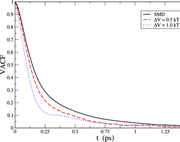
Figure 4: The normalized center of mass velocity autocorrelation function for different levels of energy terracing.

Dynamical correlations, on the other hand, tend to be more sensitive to the level of discretization in the stepped-potential. Considering the normalized autocorrelation function of the velocity of the center of mass (VACF), shown in Fig. 4, it is clear that the VACF decays too quickly for large steps. This behavior can be understood by noting that the average number of neighbors in the first solvation shell is too large when $\Delta V=kT$, as can be seen from the radial distribution functions in Fig. 3. The increase in the average number of neighbors around a given particle leads to an enhanced number of interactions at short times that give an exaggerated kick in random directions to the center of mass velocities and leads to a rapid loss of correlation. However as the energy steps are reduced, there is a convergence of the VACF towards the result of the SMD simulations since the local structure as well as the magnitude of the impulses are modified. Note that when $\Delta V=kT/2$, the life-time of velocity correlations is roughly correct.

The same trends are observed in the orientational correlation functions. As is clear from Fig. 5, the normalized autocorrelation function of the long-axis of the rods decays too slowly when the energy discontinuities are too large. Once again, the long lifetime of orientational correlations for the system with large discontinuities is indicative of pairs of molecules being too tightly bound in an orientationally dependent, locally-preferred configuration. However, the DMD results rapidly approach the SMD result as $\Delta V$ is reduced to $kT/2$ and exhibit the correct degree of anti-correlation for times around $0.15$ ps.

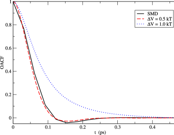
Figure 5: The normalized autocorrelation function of the long axis vector for different levels of energy terracing.

For dense systems, the event-driven simulations are not expected to be much more efficient than SMD simulations that take of advantage of stable and accurate symplectic integration schemes. The cost of the DMD simulation scales linearly with the number of events processed per picosecond of time. Interestingly, for $\Delta V$ in the range of $kT$ to $2$ $kT$, the number of interactions per picosecond is approximately constant and equal to $3.5\times 10^{4}$ coll/ps. At this rate of events, the DMD simulations are roughly $1.7$ times more efficient than the SMD simulations. However for $\Delta V=kT/2$, where the dynamics compares well with the dynamics of the continuous system, the rate of interactions per picosecond increases to around $4.7\times 10^{4}$ coll/ps and the relative efficiency of the DMD simulations drops to $1.25$. Of course these results depend strongly on a number of conditions, including the physical conditions of simulation, and are particularly sensitive to the density. For example, for a gaseous system where $T^{*}=10$ and $\rho^{*}=0.01$, the DMD simulation with $\Delta V=kT/2$ becomes more than $120$ times more efficient than the SMD simulations. From an algorithmic point of view, the low density DMD simulations resemble an adaptive time step simulation approach in which large time steps are utilized to integrate the equation of motion of a given particle when it is not interacting with any others, and when another particle is encountered, the time step is reduced to properly evolve the system through the interaction region. The energy-terracing scheme and event detection algorithm naturally provide an adaptive approach in which an interacting pair may experience many events in rapid succession as the pair evolves through an interaction region.

VI Conclusions

In this article a general framework for performing event-driven dynamics of rigid bodies has been presented that makes use of a mapping of a continuous potential onto discrete values. The evolution of the discretized-energy system consists of periods of free propagation of the system punctuated by impulses generated at discrete times that correspond to moments when the underlying continuous interaction potential for a pair of particles hits a critical value. An adaptive grid method using cubic interpolation was presented to facilitate the search for the earliest interaction time. The effect of the impulses on the subsequent dynamics of the system was analyzed using conservation conditions, resulting in a simulation algorithm that solves the evolution of the system within numerical precision. The trajectories are time-reversible, and exactly obey all applicable conservation laws by construction.

The method was demonstrated on a system of dense rigid rods interacting by a discretized version of a simple modified Lennard-Jones pair interaction potential in which the effective distance depends explicitly on the relative orientation of the rods. Although static correlations were reasonably well represented in the discretized potential system provided the energy mapping was not too coarse, dynamical correlations and related quantities such as the orientational relaxation time depend sensitively on the level of discretization of the continuous potential. It was found that potential energy steps on the order of $kT/2$ were required to reproduce results from simulations of the continuous potential system.

It should be emphasized that the implementation tested here, in which an evenly-spaced energy discretization was used, is the simplest choice of mapping of the continuous system onto a set of discrete energy levels. It is quite likely that some other distribution of energy levels would lead to substantial improvements in both the quality of the simulation results and the overall efficiency of the algorithm. However such modifications to the implementation must be carefully considered, since typically one is only interested in rough qualitative behavior of a system that is not overly sensitive to details of an interaction potential. In this case, the goal is to construct a simple model that demonstrates the relevant physics. A few, well-chosen potential energy discontinuities can be expected to meet this goal.

References

- (1) D. Frenkel and B. Smit, Understanding Molecular Dynamics (Academic Press, San Diego, California, 2004), 2nd ed.
- (2) D. C. Rapaport, J. Comp. Phys. 34, 184 (1980).
- (3) W.B. Streett, D.J. Tildesley, and G. Saville, Mol. Phys. 35, 639 (1978); M. Tuckerman, B.J. Berne, and G.J. Martyna, J. Chem. Phys. 94, 6811 (1991); R.D. Skeel and J.J. Biesiadecki, Annals of Numer. Math. 1, 191 (1994).
- (4) Y. Funato, P. Hut, S. McMillan, and J. Makino, Astrophysics Journal 112, 1697 (1996); M. Preto and S. Tremaine, Astron. J. 118, 2532 (1999).
- (5) L. Hernández de la Peña, R. van Zon, J. Schofield and S. Opps, J. Chem. Phys. 126, 074105 (2007).
- (6) J.G. Gay and B.J. Berne, J. Chem. Phys. 74, 3316 (1981).
- (7) Y. Liu and T. Ichiye, J. Phys. Chem. 100, 2723 (1996).
- (8) H. Goldstein, Classical Mechanics (Addison-Wesley, Reading, Massachusetts, 1980).
- (9) L. Hernández de la Peña, J. Schofield and S. Opps, J. Chem. Phys. 126, 074106 (2007).
- (10) R. van Zon and J. Schofield, J. Comput. Phys. 225, 145 (2007).
- (11) This symmetry is often broken in molecular simulations due to periodic boundary conditions.
- (12) W. H. Press, S. A. Teukolsky, W. T. Vetterling and B. P. Flannery, Numerical Recipes in FORTRAN: the Art of Scientific Computing, Cambridge University Press (1992).
- (13) R. P. Brent, Algorithms for Minimization without Derivatives (Englewood Cliffs, NJ: Prentice Hall).
- (14) Another way to show that the scalars have to be equal, is to note that the direction of the impulse in six dimensional configuration space (including relative orientation and position) is in the direction of the normal to the boundary of the terrace being hit. This normal is given by the gradient of the smooth underlying potential, and thus the six dimensional impulse has to have the same direction, with only a single scalar to be determined.
- (15) G. Paul, J. Comput. Phys. 221, 615 (2007).
- (16) R. van Zon and J. Schofield, Phys. Rev. E 75, 056701 (2007); R. van Zon, I. Omelyan, and J. Schofield, submitted.