Why many theories of shock waves are necessary. Kinetic functions, equivalent equations, and fourth-order models

Abstract

We consider several systems of nonlinear hyperbolic conservation laws describing the dynamics of nonlinear waves in presence of phase transition phenomena. These models admit under-compressive shock waves which are not uniquely determined by a standard entropy criterion but must be characterized by a kinetic relation. Building on earlier work by LeFloch and collaborators, we investigate the numerical approximation of these models by high-order finite difference schemes, and uncover several new features of the kinetic function associated with with physically motivated second and third-order regularization terms, especially viscosity and capillarity terms.

On one hand, the role of the equivalent equation associated with a finite difference scheme is discussed. We conjecture here and demonstrate numerically that the (numerical) kinetic function associated with a scheme approaches the (analytic) kinetic function associated with the given model — especially since its equivalent equation approaches the regularized model at a higher order. On the other hand, we demonstrate numerically that a kinetic function can be associated with the thin liquid film model and the generalized Camassa-Holm model. Finally, we investigate to what extent a kinetic function can be associated with the equations of van der Waals fluids, whose flux-function admits two inflection points.

1 Introduction

1.1 Background

In this paper we study the numerical approximation of several first-order nonlinear hyperbolic systems of conservation laws, and we consider discontinuous solutions generated by supplementing the hyperbolic equations with higher-order, physically motivated, vanishing regularization terms. Specifically, we consider complex fluid flows when physical features such as viscosity and capillarity effects can not be neglected even at the hyperbolic level of modeling, and need to be taken into account. This gives rise to many shock wave theories associated with any given nonlinear hyperbolic system: depending on the underlying small-scale physics of the problem under consideration, one need a different selection of “entropy solutions”.

It is well known that solutions of nonlinear hyperbolic equations become discontinuous in finite time, and may, therefore, exhibit shock waves. Classical shock waves satisfy standard entropy criteria (due to Lax, Oleinik, Wendroff, Liu, Dafermos, etc); they are compressible and stable under perturbation and approximation.

On the other hand, discontinuous solutions of hyperbolic problems may also exhibit non-classical, under-compressive shock waves – also referred to as subsonic phase boundaries in the context of phase transition theory. To uniquely characterize under-compressive shocks one need to impose a jump condition that is not implied by the given set of conservation laws and is called a kinetic relation. The selection of physically meaningful shock waves of a first-order hyperbolic system is determined by traveling waves associated with an augmented system that includes viscosity and capillarity effects. That is, one searches for scale-invariant solutions depending only on the variable $y:=x-\lambda\,t$ for some speed $\lambda$ and connecting two constant states $(\tau_{-},u_{-})$ and $(\tau_{+},u_{+})$ at infinity. The characterization of these “admissible” discontinuities is based on kinetic relations. (For background, see [20] and the references cited therein.)

For instance, one important model of interest in fluid dynamics describes liquid-vapor flows governed by van der Waals’s equation of state. For pioneering mathematical works on van der Waals fluids we refer to Slemrod et al. [29, 30, 13], who investigated self-similar approximations to the Riemann problem. The concept of a kinetic relation associated with (undercompressive) nonclassical shocks or phase boundaries was introduced by Abeyaratne and Knowles [1, 2], Truskinovsky [31, 32], and first analyzed mathematically by LeFloch [19]. Kinetic relations and nonclassical shocks were later studied extensively by Shearer et al. [18, 28] (phase transition), LeFloch et al. [14, 15, 16, 21, 5] (traveling waves, Riemann problem, general hyperbolic systems), and by Bertozzi, Shearer, et al. [7, 6] (thin film model), as well as Colombo, Corli, Fan, and others (see [10, 11, 12, 13] and the references cited therein).

1.2 Approximation of undercompressive waves

The present paper built on existing numerical work done by the first author and his collaborators [14, 15, 22, 8, 9] and devoted to the numerical investigation of non-classical shocks and phase boundaries generated by diffusive and dispersive terms kept in balance. These papers cover scalar conservation laws, and systems of two or three conservation laws arising in fluid dynamics (Euler equations) and material science. Entropy stable schemes were constructed, and kinetic relations were computed numerically. Numerical kinetic functions turn out to be very useful to to evaluate the accuracy and efficiency of the schemes under consideration.

Numerical experiments were also performed on undercompressive shocks for the models of thin films [6, 24, 25] and phase dynamics [26]. These authors did not investigate the role of the kinetic relation for these models, and one of our aims in the present paper is to tackle this issue.

Recall that one effective numerical strategy to compute under-compressive waves is provided by the Glimm and front tracking schemes, for which both theoretical and numerical results are now available [20, 9]. Both schemes converge to the correct non-classical solutions to any given Cauchy problem. The main feature of these schemes is to completely avoid spurious numerical dissipation or dispersion, which this guarantees their convergence to the physically meaningful solution selected by the kinetic relation. However, this class of schemes has some drawbacks: they are limited to first-order accuracy and require the precise knowledge of the Riemann solver, while numerical solutions may exhibit a noisy behavior.

In contrast, in the last twenty years, modern, high-order accurate, finite difference techniques of (classical) shock capturing have been developed to deal with discontinuous solutions of hyperbolic problems. Extending these techniques to compute nonclassical shocks turned out to be quite difficult, however. Our aim in the present paper is to pursue this investigation of the interplay between dissipative and dispersive mechanisms in hyperbolic models, and to better understand how they compare with similar mechanisms taking place in finite difference schemes.

This problem was first tackled by Hayes and LeFloch [14, 15] where the importance of the equivalent equation associated with a scheme was pointed out and kinetic functions for schemes were computed. Next, the role of high-order, entropy conservative schemes was emphasized and further kinetic functions were determined numerically [22]. In the situation just described, the numerical solutions usually contain mild oscillations, which vanish out when the mesh is refined. This feature is entirely consistent with the behavior of traveling wave solutions to the underlying dispersive model. In consequence, total variation diminishing (TVD) techniques should not be used to compute nonclassical shocks. Observe also that the diffusive-dispersive model serves only to provide a mechanism to select “admissible” solutions of associated hyperbolic equations. It has been established, for many hyperbolic models, that physically meaningful solutions can be characterized uniquely by pointwise conditions on shocks (Rankine-Hugoniot jump conditions, an entropy inequality, a kinetic relation, and, possibly, a nucleation criterion).

Finite difference schemes can also be studied for their own sake, and one important issue is whether criteria can be found for a given scheme to generate nonclassical shocks or not. Some heuristics were put forward in [15] and allow one to distinguish between the following cases:

• Schemes satisfying (a discrete version of) all of the entropy inequalities. In the context of scalar conservation laws, this is the case of the schemes with monotone numerical flux functions. For systems of two conservation laws (which admit a large family of (convex) mathematical entropies) this class includes the Godunov and the Lax-Friedrichs schemes (for small data, at least). These schemes, if convergent, must converge to a weak solution satisfying all entropy inequalities which, consequently, coincides with the classical solution selected by the Oleinik or Kruzkov entropy conditions (scalar equations) and the Wendroff or Liu entropy conditions (systems of two or more conservation laws).

• Schemes satisfying a single (discrete) entropy inequality but applied to a system with genuinely nonlinear characteristic fields. The classification of Riemann solutions given in [16] shows that, again, only the scheme can converge to the classical entropy solution, only.

• Schemes satisfying a single (discrete) entropy inequality but applied to a system with non-genuinely nonlinear characteristic fields. To decide whether such schemes are expected to generate nonclassical shocks, one should determine the equivalent equation. One may truncate the equivalent equation and keep only the first two terms. An analysis of the properties of traveling waves for this continuous model provides an indication of the expected behavior of the scheme. Interestingly, the behavior depends on the sign of the dispersion coefficient and the sign of the third-order derivative of the flux. For instance, for first-order schemes applied to scalar equations one typically obtains, after further linearization in the neighborhood of the origin $0$ in the phase space,

  $$v_{t}\pm(v^{3})_{x}=h\,v_{xx}+\alpha h^{2}\,v_{xxx}.$$

  Nonclassical shocks have been observed when the flux is concave-convex (that is, $v^{3}$) and $\alpha$ is positive, or else when the flux is convex-concave (that is, $-v^{3}$) and the coefficient $\alpha$ is negative.

1.3 Purpose of this paper

We will demonstrate here that the existence of under-compressive shocks and several typical behaviors of these nonlinear waves, especially the existence of a kinetic function, are properties shared by many examples arising in continuum physics. To make our point, we present a number of physical models describing nonlinear wave dynamics dynamics: cubic flux, thin liquid films, generalized Camassa-Holm, van der Waals fluids. Specifically, we prove that kinetic functions can be associated to each of these models and we study their monotonicity, dependence upon (viscosity, capillarity, mesh) parameters, and behavior in the large. We uncover several new features of the kinetic function that have not been observed theoretically via analytical methods yet. It is our hope that the conclusions reached here numerically will motivate further theoretical developments in the mathematical theory of non-classical shocks. The work also provides further ground that not a single theory of entropy solutions but, rather, many theories of shock waves are required to accurately describe singular limits of hyperbolic equations, as supported by the framework developed in [20, 21, 23].

The outline of the paper is as follows. In Section 2, we present the physical models of interest and discuss briefly their analytical properties. In Section 3, after introducing some background on non-classical shocks and kinetic relations, we investigate the role of the equivalent equation. In Section 4, we establish the existence of kinetic functions associated with each of the models and investigate their properties. In Section 5, we investigate van der waals fluids. Finally, Section 6 contains concluding remarks.

2 Models of interest

We begin with a brief presentation of a few nonlinear hyperbolic models arising in continuum physics.

2.1 Cubic conservation law

It will be convenient to start with an academic example consisting of a conservation law whose flux-function admits a non-degenerate inflection point. For simplicity and with little loss of generality as far as the local behavior near the inflection point is concerned, we can assume that the flux is a cubic function. After normalization, we arrive at the cubic conservation law

$$u_{t}+(u^{3})_{x}=0,\quad u=u(t,x)\in{I\!\!R},\,t\geq 0.$$ (2.1)

We are interested in (discontinuous) solutions that can be realized as limits of diffusive-dispersive solutions of

$$u_{t}+(u^{3})_{x}=\epsilon\,u_{xx}+\alpha\,\epsilon^{2}\,u_{xxx},\quad u=u_{\alpha}^{\epsilon}(t,x),$$ (2.2)

where $\alpha$ is a fixed parameter and $\epsilon\to 0$. Recall that shock waves of (2.1) are solutions containing a single propagating discontinuity connecting two states $u_{-},u_{+}$ at the speed $\lambda$. These constants must satisfy the Rankine-Hugoniot relation

$$\lambda={u_{+}^{3}-u_{-}^{3}\over u_{+}-u_{-}}=u_{-}^{2}+u_{-}\,u_{+}+u_{+}^{2},$$

as well as the entropy inequality associated with the quadratic entropy ${U(u):=u^{2}}$

$$-\lambda\,(u_{+}^{2}-u_{-}^{2})+{2\over 3}\,(u_{+}^{4}-u_{-}^{4})\leq 0.$$

As is now well-known, the solutions $u_{\alpha}:=\lim_{\epsilon\to 0}u^{\epsilon}_{\alpha}$ may contain both classical shock waves satisfying the standard compressibility condition (equivalent here to the entropy criteria introduced by Lax)

$$3\,u_{-}^{2}=f^{\prime}(u_{-})\geq\lambda\geq f^{\prime}(u_{+})=3\,u_{+}^{2},$$ (2.3)

as well as non-classical shock waves which turn out to be under-compressive

$$\lambda<f^{\prime}(u_{\pm}).$$ (2.4)

The characterization of the solutions generated by (2.2) as $\epsilon\to 0$ is provided as follows. Based on an analysis of all possible traveling wave solutions of (2.2), one can see that, for a given viscosity/capillarity ratio $\alpha$ and for every left-hand state $u_{-}$, there exists a single right-hand state

$$u_{+}=\varphi^{\flat}_{\alpha}(u_{-}),$$ (2.5)

that can be attained by a non-classical shock. The function $\varphi^{\flat}_{\alpha}$ is called the kinetic function associated with the model (2.2). The existence of the kinetic function has been established theoretically for a large class of flux-functions and nonlinear diffusion-dispersion operators, including (2.2). The results are often stated in terms of the shock set, ${\mathbf{S}}_{\alpha}(u_{-})$, consisting of all right-hand states $u_{+}$ that can be attained from a given left-hand state $u_{-}$ by a classical or by a non-classical shock. Note also that instead of the relation (2.5), one can equivalently prescribe the entropy dissipation of a non-classical shock, that is the kinetic relation can be expressed in the following form observed in [19]:

$$-\lambda\,(U(u_{+})-U(u_{-}))+F(u_{+})-F(u_{-})$$ (2.6)

$$=-\int_{I\!\!R}U^{\prime\prime}(v(y))\,v_{y}(y)^{2}\,dy\leq 0,$$

where $y\mapsto v(y)$ denotes the traveling wave trajectory connecting $u_{-}$ to $u_{+}$. In orther words, the entropy dissipation must be prescribed on a non-classical shock. As far as the specific model with cubic flux and linear diffusion and dispersion is concerned, the kinetic function and the shock set can be expressed explicitly by analytical formulas as follows. The kinetic function associated with (2.2) reads

$$\varphi^{\flat}_{\alpha}(u_{-})=\begin{cases}-u_{-}-{\tilde{\alpha}}/2,&u_{-}\leq-{\tilde{\alpha}},\\ -u_{-}/2,&|u_{-}|\leq{\tilde{\alpha}},\\ -u_{-}+{\tilde{\alpha}}/2,&u_{-}\geq{\tilde{\alpha}},\end{cases}$$ (2.7)

with ${\tilde{\alpha}}:=\sqrt{(8/3\alpha)}$, while the corresponding shock set is

$${\mathbf{S}}_{\alpha}(u_{-})\,=\,\begin{cases}(u_{-},{\tilde{\alpha}}/2]\cup\big{\{}-u_{-}-{\tilde{\alpha}}/2\big{\}},&u_{-}\leq-{\tilde{\alpha}},\\ [-u_{-}/2,u_{-}),&-{\tilde{\alpha}}\leq u_{-}\leq{\tilde{\alpha}},\\ \big{\{}-u_{-}+{\tilde{\alpha}}/2\big{\}}\cup[-{\tilde{\alpha}}/2,u_{-}),&u_{-}\geq{\tilde{\alpha}}.\end{cases}$$

Observe that $\varphi^{\flat}_{\alpha}$ converges to $-u/2$ when $\alpha\to 0$, and that the shock set converges to the standard interval $[-u/2,u]$ determined by the Oleinik entropy inequalities. See [20] for details.

2.2 Thin liquid films

The thin liquid film model ($\epsilon,\alpha$ being positive, scaling parameters)

$$u_{t}+(u^{2}-u^{3})_{x}=\epsilon\,(u^{3}\,u_{x})_{x}-\alpha\epsilon^{2}\,(u^{3}\,u_{xxx})_{x}$$ (2.8)

describes the dynamics of a thin film with height $u=u(t,x)$ moving on an inclined flat solid surface. The (non-convex) flux-function

$$f(u)=u^{2}-u^{3},\quad 0\leq u\leq 1,$$

represents the competing effects of the gravity and a surface stress known as the Marangoni stress. The latter arises in experiments due to an imposed thermal gradient along the solid surface. The fourth-order diffusion is due to surface tension, and the second-order diffusion represents a contribution of the gravity to the pressure. This model was introduced and extensively studied by Bertozzi, Münch, and Shearer [6]. The existence of non-classical traveling waves was established analytically in [7], and various numerical studies were performed [25, 24] which exhibited subtil properties of stability and instability of these waves. For more analytical background, see also the convergence theory developed by Otto and Westdickenberg [27].

From the standpoint of the general well-posedness theory the kinetic relation is an important object which is necessary to uniquely characterized the physically meaningful solutions. A kinetic function was not exhibited in the work [7] which, instead, relied on non-constructive arguments. From the existing literature, it is not clear whether a concept of a kinetic relation could be associated with the equation (2.8) and, if so, and whether such a kinetic function would enjoy the same monotonicity properties, as the ones established earlier for conservation laws regularized by viscosity and capillarity. This issue will be addressed in Section 4.

Observe that the flux $f(u)$ here is positive on the interval $(0,1)$, increasing on $(0,2/3)$ and decreasing on $(2/3,1)$. It admits a single inflection point at $u=1/3$. To every point $u\in(0,1/3)$ we can associate the “tangent point” $\varphi(u)\in(1/3,1/2)$ characterized by

$$f^{\prime}(\varphi^{\natural}(u))={f(u)-f(\varphi^{\natural}(u))\over u-\varphi^{\natural}(u)},$$

or

$$\varphi^{\natural}(u):={1-u\over 2}.$$

The same formula maps also the interval $(1/3,1)$ onto $(0,1/3)$. This function $\varphi^{\natural}$ allows us to define classical shock waves associated with the equation. When $u\in(0,1/3)$ the left-hand state $u$ can be connected to the right-hand state $\varphi^{\natural}(u)$ by a contact discontinuity. When $u\in(1/3,1)$, $\varphi^{\natural}(u)$ is the left-hand state and $u$ is the right-hand state.

Another important function is provided by considering the entropy dissipation

$$D(u_{-},u_{+}):=-{\lambda\over 2}(u_{+}^{2}-u_{-}^{2})+{2\over 3}(u_{+}^{3}-u_{-}^{3})+{3\over 4}(u_{+}^{4}-u_{-}^{4}).$$

where the shock speed $\lambda$ is given by

$$\lambda:={f(u_{+})-f(u_{-})\over u_{+}-u_{-}}=u_{+}+u_{-}-(u_{+}^{2}+u_{+}u_{-}+u_{-}^{2}).$$

The zero dissipation function $\varphi^{\sharp}$ is by definition the non-trivial root of $D$, i.e.

$$D(u,\varphi^{\sharp}(u))=0,$$

or

$$\varphi^{\sharp}(u):={2\over 3}-u.$$

The function $\varphi^{\sharp}$ maps the interval $(0,2/3)$ onto itself.

According to the theory in [20] the range of the nonclassical shocks is limited by the functions $\varphi^{\natural}$ and $\varphi^{\sharp}$. Precisely, for a nonclassical shock connecting $u_{-}<1/3$ to $u_{+}>1/3$, the right-hand state must have

$$\varphi^{\natural}(u_{-})={1-u_{-}\over 2}\leq u_{+}<\varphi^{\sharp}(u_{-})={2\over 3}-u_{-}.$$

The sign are reversed for a decreasing nonclassical shock.

2.3 Generalized Camassa-Holm model

We consider a generalized version of the Camassa-Holm equation

$$u_{t}+f(u)_{x} =\epsilon\,u_{xx}+\alpha\epsilon^{2}\big{(}u_{xxt}+2\,u_{x}u_{xx}+uu_{xxx}\big{)},$$ (2.9)

$$=\epsilon\,u_{xx}+{\alpha\over 2}\epsilon^{2}\big{(}2u_{xt}+(u^{2})_{xx}-(u_{x})^{2}\big{)}_{x},$$

which arises as an asymptotic higher-order model of wave dynamics in shallow water. The second-order and third-order terms are related to the viscosity and the capillarity of the fluid. When the flux $f$ is nonconvex, for instance

$$f(u)=u^{3}$$

nonclassical shocks may in principle arise. We will demonstrate in this paper that indeed solutions may exhibit nonclassical shocks and establish the existence of an associated kinetic function.

2.4 Van der Waals fluids

Compressible fluids are governed by the following two conservation laws:

$$\begin{split}&\partial_{t}\tau-\partial_{x}u=0,\\ &\partial_{t}u+\partial_{x}p(\tau)=\epsilon\partial_{xx}u-\alpha\,\epsilon^{2}\partial_{xxx}\tau.\end{split}$$ (2.10)

Here, $u$ and $\tau$ represent the velocity and the specific volume of the fluid, respectively, while $\alpha$ is a non-negative parameter representing the strength of the viscosity. The pressure law $p=p(\tau)$ is a positive function defined for all $\tau\in(0,+\infty)$ and of the following van der Waals type: there exist $0<a<c$ such that

$$\begin{split}&p^{\prime\prime}(\tau)>0,\quad\tau\in(0,a)\cup(c,+\infty),\\ &p^{\prime\prime}(\tau)<0,\quad\tau\in(a,c),\\ &p^{\prime}(a)>0,\end{split}$$ (2.11)

and

$$\lim_{\tau\to 0}p(\tau)=+\infty,\qquad\lim_{\tau\to+\infty}p(\tau)=0.$$ (2.12)

The left-hand side of (2.10) forms a first-order system of partial differential equations, which is of elliptic type when $\tau$ belongs in the interval $(d,e)$ characterized by the conditions $0<d<a<e<c$ and $p^{\prime}(d)=p^{\prime}(e)=0$. It is of hyperbolic type when $\tau\in(0,d)\cup(e,+\infty)$ and admits the two (distinct, real) wave speeds $\pm\sqrt{-p^{\prime}(\tau)}$.

3 A conjecture on the equivalent equation

3.1 Kinetic functions associated with difference schemes

We now begin the discussion of the numerical approximation of the solution $u_{\alpha}$ generated by (2.2). The discussion applies to general conservation laws of the form

$$\partial_{t}u+\partial_{x}f(u)=0,$$

where the flux-function $f$ admits a single inflection point. To any finite difference scheme associated with (2.1) one can in principle associate a kinetic function, which we denote by $\psi^{\flat}_{\alpha}$. It may seem natural to request that $\psi^{\flat}_{\alpha}$ coincides with the kinetic function $\varphi^{\flat}_{\alpha}$ associated with the given model. However, it has been observed by Hayes and LeFloch [15] that, at least for all finite difference schemes that have been considered so far,

$$\psi^{\flat}_{\alpha}\neq\varphi^{\flat}_{\alpha}.$$ (3.1)

This discrepancy is due to the fact that the dynamics of non-classical shocks is determined by small-scale features of the continuous model (2.2) which can never be fully mimicked by a discrete model.

Given this perspective, the next natural question is to compare the kinetic functions $\psi^{\flat}_{\alpha}$ and $\varphi^{\flat}_{\alpha}$. We require that a scheme be a good approximation of the given, continuous model in the following sense. Its equivalent equation obtained by formal Taylor expansion should have the “correct” form

$$v_{t}+(v^{3})_{x}=\epsilon\,v_{xx}+\alpha\,\epsilon^{2}\,u_{xxx}+O(h^{q}),\quad h=c\,\epsilon,$$ (3.2)

where $c$ is a constant and $q$ represent the order of accuracy of the scheme. Here, $v$ denotes the numerical solution and $h$ denotes the discretization parameter. It is important to observe that all of the schemes considered in the present paper are first-order accurate, only, as far as the hyperbolic equation (2.1) is concerned. They are, however, high-order approximations of the augmented model (2.2). For clarity, we emphasize the dependence in $q$ and denote by $\psi^{\flat,q}_{\alpha}$ the kinetic function associated with a scheme whose equivalent equation is (3.2).

Let us introduce in this paper the following:

Conjecture 3.1

As $q\to\infty$ the kinetic function $\psi^{\flat,q}_{\alpha}$ associated with a scheme with equivalent equation (2.7) converges to the exact kinetic function $\varphi^{\flat}_{\alpha}$,

$$\lim_{q\to\infty}\psi^{\flat,q}_{\alpha}=\varphi^{\flat}_{\alpha}.$$ (3.3)

Rigorous results pointing toward the validity of this conjecture can be found in [4] which studies the role of relaxation terms in traveling wave solutions of conservation laws. A closely related problem was tackled by Hou and LeFloch [17] who considered nonconservative schemes for the computation of nonlinear hyperbolic problems. In these problems, small-scale features are critical in selecting shock waves, and the equivalent equation have been found to provide a guide to designing difference schemes. We will not try here to support the above conjecture on theoretical grounds, but we propose to investigate it numerically. As we will see, very careful experiments are necessary. We consider a large class of schemes based on standard differences, and obtained by approximating the spatial derivatives arising in (2.2) –with $\epsilon$ replaced by the mesh size $h$ (up to a constant multiplicative factor)–

$$f(u)_{x},\quad h\,u_{xx},\quad h^{2}\,u_{xxx},$$

by high-order finite differences, so that the overall scheme is of order $q$ at least. For completeness we list below the corresponding expressions. We denote by $x_{i}$ the points of spacial mesh and by $u_{i}$ the approximation of the solution at the point $x_{i}$. We also use the notation $f_{i}:=f(u_{i})$.  Based on the above we arrive at semi-discrete schemes for the functions $u_{i}=u_{i}(t)$. For instance, using fourth order discretizations above we obtain

$$\begin{split}{du_{i}\over dt}=&-{1\over h}\,\Big{(}{1\over 12}f_{i-2}-{2\over 3}f_{i-1}+{2\over 3}f_{i+1}-{1\over 12}f_{i+2}\Big{)}\\ &+{\epsilon\over h}\,\Big{(}-{1\over 12}u_{i-2}+{4\over 3}u_{i-1}-{5\over 2}u_{i}+{4\over 3}u_{i+1}-{1\over 12}u_{i+2}\Big{)}\\ &+{\alpha\,\epsilon^{2}\over h}\,\Big{(}-{1\over 2}u_{i-2}+u_{i-1}-u_{i+1}+{1\over 2}u_{i+2}\Big{)}.\end{split}$$ (3.4)

Observe that this is a fully conservative scheme, in the sense that $\sum_{i}u_{i}(t)$ is independent of $t$ (assuming, for instance, periodic boundary conditions).  To actually implement the above algorithm, we use a Runge-Kutta scheme. Defining $U(t)=(u_{i}(t))$ (with ${i=\ldots,-1,0,1,\ldots}$), the semi discrete scheme takes the form

$${dU\over dt}(t)=R[U(t)],$$ (3.5)

where $R[U(t)]$ represents the spatial discretization. This system of ordinary differential equations is solved numerically by employing an $s$-stage Runge-Kutta scheme defined as follows

$$\begin{split}&g^{k}=R\Big{(}U^{n}+\Delta t\,\sum_{j=1}^{k-1}a_{k,j}\,g^{j}\Big{)},\\ &U^{n+1}:=U^{n}+\Delta t\,\sum_{k=1}^{s}b_{k}\,g^{k}.\end{split}$$ (3.6)

For example, the non-zero coefficients of the fourth-order Runge-Kutta scheme are given by

$$a_{2,1}=1/2,a_{3,2}=1/2,a_{4,3}=1,$$ (3.7)

$$b_{1}=1/6,b_{2}=1/3,b_{3}=1/3,b_{4}=1/6.$$

Coefficients of a sixth and an eighth-order Runge-Kutta scheme are found in [33] and [34], respectively.

3.2 Numerical experiments

We now determine numerically the kinetic function associated with the schemes described in the previous section. For each $q=4,6,8,10$ and for selected values of the parameter $\alpha$ we compute the function $\psi^{\flat,q}_{\alpha}$. For the cubic flux function, two typical types of non-classical waves arise, which are under-compressive shock followed by a rarefaction wave (Figure 1, left), and a double shock structure (Figure 1, right).

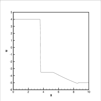
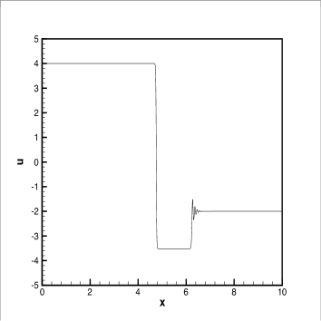
Figure 1: Typical cases of non-classical waves for the cubic flux function.

In order to plot a single kinetic function it is necessary to solve a large number of Riemann problems for various values of left-hand state $u_{-}$ and to ensure that the right-hand state is picked up in an interval where a non-classical shock does exist. In the numerical experiments it is often convenient to select the right-hand state so that the Riemann solution contain two shocks. According to the construction algorithm in [21] the middle state between the two shocks is therefore the kinetic value $u_{+}=\psi^{\flat,q}_{\alpha}(u_{-})$.

Several difficulties arise. First, when $u_{-}$ is close to the origin all the waves become very weak and it is numerically difficult to identify the middle state. Second, in a range of parameter values, the two waves may propagate with speeds that are very close and this again makes difficult the computation of the middle state. Finally, solutions do contain mild oscillations, especially for small values of $\alpha$ and this again introduces some numerical error. Due to these constraints we need to use a rather fine mesh, with $h$ of the order of $1/1000$.

The following plots allow us to investigate numerically the convergence of the kinetic function $\psi^{\flat,q}_{\alpha}$ toward the exact kinetic function, (2.7), which is a piecewise affine function of the variable $u_{-}$.

In the following numerical tests, the CFL number was taken to be as large as possible in each run and was identical for all schemes (4th order to 10th order). It was observed that increasing the order of Runge-Kutta scheme (in the temporal integration) from four to six and eighth practically does not change the results, therefore, a tenth order Runge-Kutta scheme was not examined. On the other hand, the order of spatial discretization was found to be very important and effectively made an important difference.

First of all, Figure 2 shows the right-hand state $u_{+}$ versus the parameter $\alpha$ for different schemes. Here, we have used $h=0.001$, $u_{-}=10$, and $\epsilon=5h$. As $\alpha$ increases, the results of different order numerical schemes become closer and closer to the exact solution. For large values of $\alpha$, e.g. $\alpha>10$, even the fourth-order scheme gives satisfactory results. Since the solution of (2.1) is, in fact, the limit of diffusive-dispersive solutions of (2.2), with $\alpha$ fixed and $\epsilon\to 0$, we conclude that (provided $\alpha$ is sufficiently large) even the fourth order scheme converges to the exact solution. Figure 2 shows also that, for a fixed value of $\alpha$ (sufficiently large), as the order of accuracy increases, the numerical solution converges to the exact one. These results strongly support Conjecture 3.1.

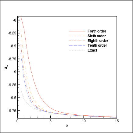
Figure 2: $u_{+}$ versus $\alpha$ for different schemes.

Next, Figure 3 (left column) shows $u_{+}$ versus $u_{-}$ for $\alpha$=1, 4 and 6 respectively, with $h=0.005$, and $\epsilon=5h$. A grid of $2000$ nodes was used in all runs. Again, by increasing the order of accuracy, the numerical solution converges to the exact one, for sufficiently small left-hand state $u_{-}$. However, the suitable value of $\alpha$ depends on $u_{-}$ and increases as $\alpha$ does. It should be mentioned that very high values of $\alpha$ (which are in need for large $u_{-}$), are not satisfactory since they lead to high oscillatory results (recall that $\alpha$ is dispersion-diffusion ratio). It was also observed that for small values of $\alpha$, high frequency oscillations occur before the non-classical shock, while for large values of $\alpha$, low frequency oscillations take place after the rarefaction (not shown).

Finally, Figure 3 (right column) shows the scaled entropy dissipation $\phi(s)/s^{2}$ versus the shock speed $s$ for $\alpha=1,4,6$, respectively. We use the quadratic entropy $U(u)=u^{2}/2$ in computing the entropy dissipation. In terms of $u_{-}$ and $u_{+}$, this is

$$\phi(u_{-},u_{+})=(u_{+}-u_{-})^{2}(u_{+}^{2}-u_{-}^{2}),$$ (3.8)

and from the Runkine-Hugoniot relation, the shock speed is

$$s=u_{-}^{2}+u_{-}u_{+}+u_{+}^{2}.$$ (3.9)

The same feature is observed as before and by increasing the order of accuracy; the numerical entropy dissipation converges to the exact one (provided $\alpha$ is sufficiently large), which is in accordance with Conjecture 3.1.

	$u_{+}$ versus $u_{-}$	$\phi(s)/s^{2}$ versus $s$
$\alpha$=1
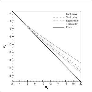
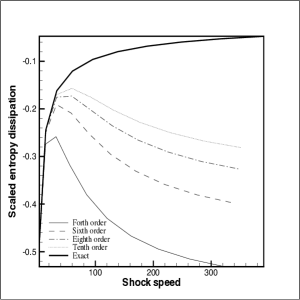
$\alpha$=4
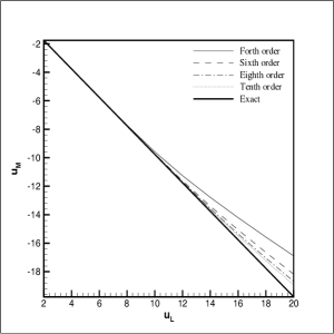
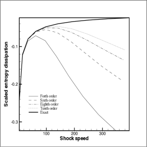
$\alpha$=6

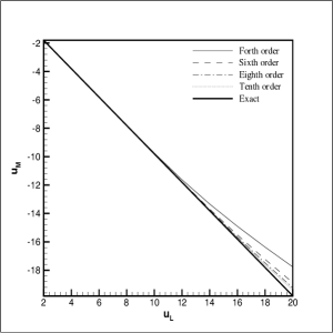
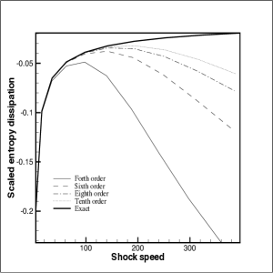
Figure 3: $u_{+}$ versus $u_{-}$ (left) and scaled entropy dissipation $\phi(s)/s^{2}$ versus shock speed $s$ (right) for different values of $\alpha$.

3.3 Spatial discretization parameter versus diffusive-dispersive parameters

To conclude this section let us set $h=c\,\epsilon$ and plot the corresponding numerical results with the sixth-order scheme and some fixed values of $h$ and $\epsilon$. It was observed that when $c$ is either too small or too large, the numerical results deteriorate and an approximate kinetic function can no longer be associated with the numerical approximations.

As shown in Figure 4 for typical values $u_{-}=10$, $\alpha=1$ and CFL=0.5, the specific choice of $c$ does not change the general feature of the results. However, as we increase the value of $c$, all schemes converge to the exact solution and the tenth order scheme converges faster. Moreover, it is concluded from Figure 4 that the sixth order scheme with $c=10$ is a reasonable choice in terms of accuracy and computational efficiency. For this value of $c$ (that is, $\epsilon=10h$) with $h=0.005$, Figure 5 shows the kinetic function $u_{+}$ versus $u_{-}$ (left) and the corresponding scaled entropy dissipation $\phi(s)/s^{2}$ versus the shock speed $s$ for $\alpha=1,4,6$ (right) which are in accordance with the previous results about the convergence of the numerical results to the exact one.

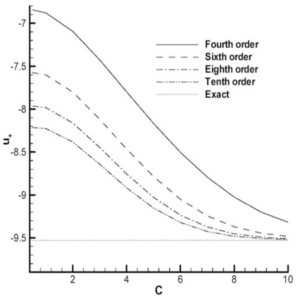
Figure 4: $u_{+}$ versus $c$ for different schemes.

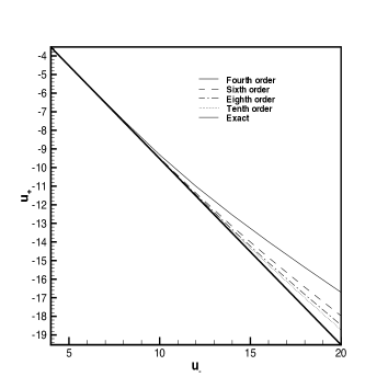
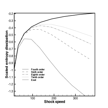
Figure 5: $u_{+}$ versus $u_{-}$ (left) and scaled entropy dissipation $\phi(s)/s^{2}$ versus shock speed $s$ (right) for $\alpha=1$ and $c=10$.

4 Fourth-order models

We now return to the examples of Section 2 and discuss the thin film and Camassa-Holm models. We will show that solutions of the Riemann problem may admit under-compressive shocks, and we will determine the corresponding kinetic function in a significant range of data. Our results in the previous section indicate that we can continue this investigation with six-order schemes, which we will do in (most of) the forthcoming tests.

4.1 Thin liquid films

Consider the model of thin liquid films together with the physical regularization terms. Our goal is to (numerically) compute a kinetic function associated with this model. It should be reminded that the physically relevant range for the solutions is the interval $(0,1)$. This model has a flux with a single inflection point, as is the case with the cubic conservation laws, and the interesting aspect is the particular form of the regularization. In view of experiments performed in [7], it may be anticipated that a unique Riemann solver can not be associated to a given set of initial data, and that the specific initialization adopted in implementing a given scheme may play a role. We will first show that a kinetic relation can be associated to a family of initial data and a given approximation of these initial data.

Since the flux has a convex-concave shape rather than a concave-convex form (contrary to the cubic flux function), the nonclassical shock is fast undercompressive and it is more convenient to draw the kinetic functions from right to left, that is,

$$u_{-}=\varphi(u_{+}).$$

The calculations here are more delicate than those performed with the third-order regularization, since we are now dealing with a fourth-order regularization. Therefore, for the discretization of the terms arising in (2.8), a scheme must be fifth order in accuracy at least. We thus exclude the fourth-order scheme used earlier and we concentrate attention on the sixth-order scheme.

It should be mentioned that the (fourth-order) regularization is singular at $u=0$, so tests involving values close to $u=0$ are challenging and the kinetic function should have some degenerate behavior as some values in the solution approache $u=0$.

The thin film model (2.8) may be written in the conservative form

$$u_{t}+g(u)_{x}=0,$$ (4.1)

with

$$g(u):=u^{2}-u^{3}-u^{3}\,(\delta\,u_{x}-\,u_{xxx}),$$ (4.2)

where we have set $\epsilon=\delta$ and $\alpha\epsilon^{2}=1$.

The numerical solution of (4.1) is obtained by calculating the terms $u_{x}$ and $u_{xxx}$ in (4.2) using the sixth order scheme (Appendix A), computing the nodal values of $g$, and finally calculating $g_{x}$ again using the sixth order scheme (Appendix A). The numerical experiments are performed here with $\delta=0.1h$ and $h=1$ using a computational grid of $1000$ nodes and the initial condition used in [7]

$$u(x)=(\tanh(-x+100)+1){(u_{L}-u_{R})\over 2}+u_{R}.$$ (4.3)

The numerical solutions of (4.1) for $u_{R}=0.1$ and $u_{L}=0.5$ and $0.6$ with $\Delta t=0.6481$ at time $t=1037$ are shown in Figure 6. For the case $u_{L}=0.5$ a double shock structure is observed while for $u_{L}=0.6$ a rarefaction wave and an under-compressive shock are generated. The speed of the non-classical shock is similar for the two cases, as expected.

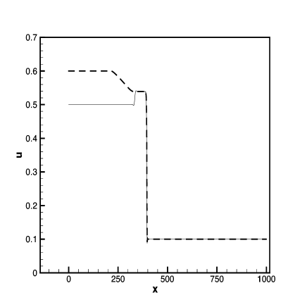
Figure 6: Wave structure for $u_{R}=0.1$ and $u_{L}=0.5$ and $0.6$.

In agreement with what was observed (and proven rigorously in [5]) for the diffusive-dispersive regularizations, when $0.2<u_{R}<0.4$, i.e. around the inflection point $u=1/3$, only classical waves are observed as shown e.g. in Figure 7 for $u_{R}=0.3$ and different values of $u_{L}$ (with $\Delta t=0.388$ at time $t=698$).

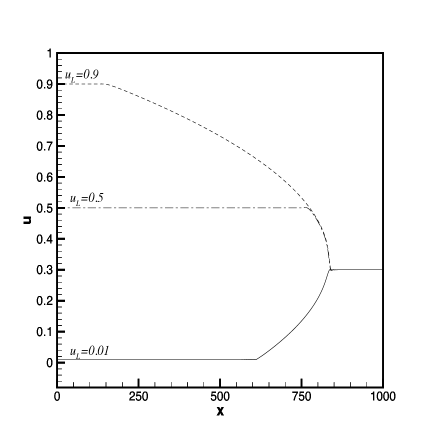
Figure 7: Wave structure for $u_{R}=0.3$ and various values of $u_{L}$.

For $0.4<u_{R}$ non-classical waves arise even when $u_{L}$ is small and become clearly visible as $u_{R}$ increases as shown in Figure 8.

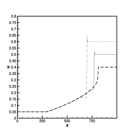
Figure 8: Wave structure for $u_{L}=0.05$ and $u_{R}=0.4$, 0.5 and $0.6$.

Figure 9 shows the numerical solutions obtained for $\Delta t=0.37$, at time $t=2148$ for $u_{R}=0.6$ and two cases $u_{L}=0.1$ and $u_{L}=0.2$. For the case $u_{L}=0.2$ a double shock structure is observed while for $u_{L}=0.1$ a rarefaction wave and an under-compressive shock are generated. It should be mentioned that when $u_{L}$ is selected large enough, only classical waves are observed as shown for $u_{L}=0.5$ and $0.68$ (with the same data) in Figure 10.

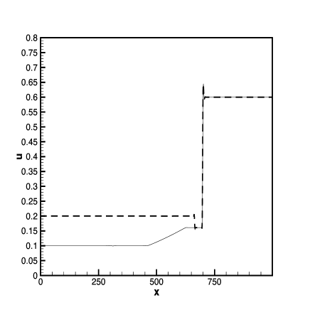
Figure 9: Wave structure for $u_{R}=0.6$ and $u_{L}=0.1$ and $0.2$.

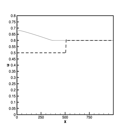
Figure 10: Wave structure for $u_{R}=0.6$ and $u_{L}=0.5$ and $0.68$.

Varying the left-hand and right-hand initial states and keeping fixed all other parameters, for $\delta=\eta h$ with $\eta=$ 0.1 we obtain the numerical kinetic function ($u_{-}$ as a function of $u_{R}$) shown in Figure 11 (left). Interestingly enough, this function is decreasing, as required in the general theory of nonclassical shocks. It is also observed that the numerical kinetic functions converge as the order of the accuracy of the numerical scheme is increased. Note that, for sufficiently large right-hand values of $u_{R}$, negative left-hand values $u_{-}$ are obtained which are physically irrelevant. The scaled entropy dissipation $\phi(s)/s^{2}$ versus the shock speed $s$ is also shown in Figure 11 (right).

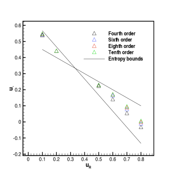
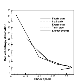
Figure 11: Kinetic function (left) and scaled entropy dissipation (right), for $\eta=0.1$ based on the initial conditions (4.3).

Finally, we study the effect of $\eta=\delta/h$ for $u_{r}=0.8$. Figure 12 presents a sample of the solution with various schemes for $\eta=4.7$. In Figure 13, it is shown that by increasing $\eta$, the numerical results converge to the limiting value with the tenth order scheme. The optimum value of $\eta$ depends on $u_{r}$ and it is increased as $u_{r}$ does (not shown). In Figure 14 we have plotted the kinetic functions for various schemes where a variable (optimum) $\eta$ (depending on $u_{r}$) is employed. The convergence predicted in Conjecture 3.1 is clearly confirmed here.

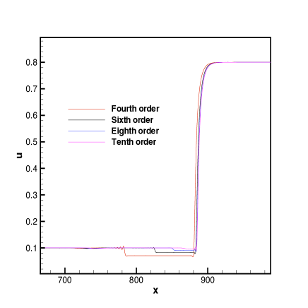
Figure 12: A sample of the solution with various schemes for $u_{r}=0.8$ and $\eta=4.7$.

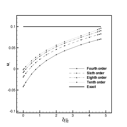
Figure 13: $u_{-}$ versus $\eta=\delta/h$ for $u_{r}=0.8$.

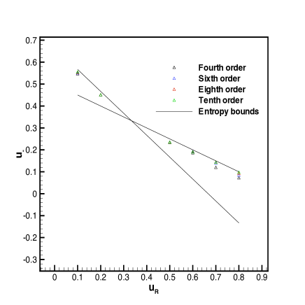
Figure 14: Kinetic function for thin films, based on the initial conditions (4.3) with optimum $\eta$.

In order to investigate the effect of the initial conditions, we consider the following initial condition

$$u(x)=\begin{cases}(0.35-u_{L})\tanh(x-80)/2+(0.35+u_{L})/2,&x\leq 105,\\ (u_{R}-0.35)\tanh(x-130)/2+(0.35+u_{R})/2,&x>105.\end{cases}$$ (4.4)

The numerical solutions of (4.1) for $u_{R}=0.7$ and $u_{L}=0.05$ with $\Delta t=0.27$ and $\Delta x=1$ at time $t=18792$ are shown in Figure 15. As shown in Figure 15, the two choices of numerical solutions lead to different results. However, such a dependence on the initial data is only limited to few cases.

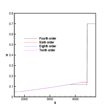
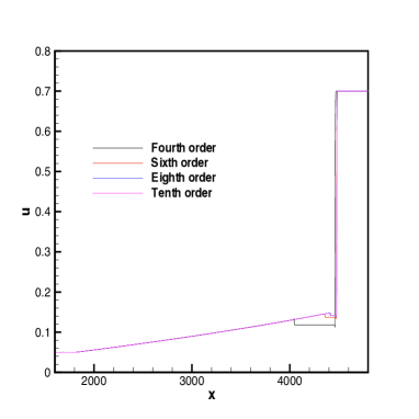
Figure 15: Numerical results obtained using the initial conditions (4.3) (left) and (4.4)(right).

4.2 Generalized Camassa-Holm model

It is expected that the kinetic function of the Camassa-Holm model is qualitatively similar to that of the diffusive-dispersive model. However, some differences, at least quantitatively are expected. In the following, we draw a kinetic function for the Camassa-Holm model and compare with the diffusive-dispersive model with the same coefficients. First, we investigate the behavior of the function for large values of $u$.

Figure 16 shows the results obtained with $h=1$, $\epsilon=0.005h$, $\alpha=1$ and CFL=0.5 using a computational grid of $1000$ nodes. The kinetic function for the Camassa-Holm model (Figure 16, right) is larger than the linear diffusion-dispersion case (Figure 16, left).

The comparison between the Camassa-Holm model and the linear diffusion-dispersion model allows to see that the kinetic function of the two models is similar for small values of $u$ but different for large values of $u$. Typically, for large values of $u$, the Camassa-Holm model leads to larger kinetic values. This behavior is due to the nonlinearity of the regularization in the right-hand side of (2.9). It would be interesting (and challenging) to apply the techniques in [5] and prove the existence and monotonicity of the kinetic function associated with the Camassa-Holm model.

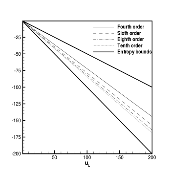
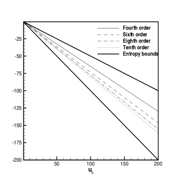
Figure 16: The kinetic function (large values of $u$) for the linear diffusion-dispersion case (left) and Camassa-Holm model (right).

We then consider small values of $u$. Figure 17 shows the results obtained for both models with $h=1$, $\epsilon=0.1h$, $\alpha=4$ and CFL=0.5 using a computational grid of $1000$ nodes. Contrary to the case of large values of $u$, the behavior of the function for small values of $u$ is the same for both models.

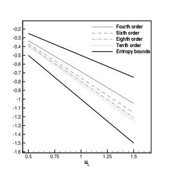
Figure 17: The kinetic function (small values of $u$) for the linear diffusion-dispersion case and Camassa-Holm model.

5 Kinetic functions associated with van der Waal fluids

Our next objective is to investigate the properties of non-classical solutions to hyperbolic conservation laws whose flux-function admits two inflection points. We consider the phase transition model (2.10) presented in Section 2. As we will see, the dynamics of non-classical shock waves for general flux is much more intricate than the now well-understood case of a single inflection point. In particular, we demonstrate numerically that the Riemann problem may well admit arbitrarily large number of solutions. This happens only when the flux admits two inflection points at least and provided the dispersion parameter is sufficiently large. We then determine the kinetic function and observe its lack of monotonicity.

We consider an equation of state having the same shape as that of van der Waals fluids, described by the (normalized) equation

$$p(\tau):={1\over(3\tau-1)^{1+1/\zeta}}-{3\over\tau^{2}},\quad u>1/3,$$ (5.1)

for some positive constant $\zeta=1/(\gamma-1)$ where $\gamma\in(1,2)$.

To exhibit the dynamics of non-classical shocks for general flux, we solve the Riemann problem for left- and right-data:

1. First, we determine the wave structure of the solution for each fixed left-hand state, that is, we identify the waves (classical/non-classical shock or rarefaction) within the Riemann solution. In turn, by varying the left-hand state, we identify regions in the plane in which the structure of the Riemann solution remain unchanged as we change the Riemann data. This provides us with a representation of the Riemann solver in the plane.

2. Second, within the range of $u_{l}$ where non-classical shocks leaving from $u_{l}$ are available, we determine the corresponding kinetic functions that are needed to characterize the dynamics of non-classical shocks. It is expected that more than one kinetic function will be needed in some range of $u_{l}$, but a single kinetic function maybe sufficient in certain intervals.

To begin with, we consider a simplified case

$$\begin{split}&\partial_{t}\tau-\partial_{x}u=0,\\ &\partial_{t}u+\partial_{x}p(\tau)=\epsilon\,\partial_{xx}u,\end{split}$$ (5.2)

with

$$p(\tau):={RT\over(\tau-\frac{1}{3})}-\displaystyle{3\over\tau^{2}},$$ (5.3)

and $R=\frac{8}{3}$ and $T=1.005$. This flux function has two inflection points at $\tau=1.00996$ and 1.8515 and it is shown in Figure 18.

In order to investigate possible wave cases, various test cases are performed by keeping three of four variables ($u_{L}$, $\tau_{L}$, $\tau_{R}$ and $u_{R}$) constant and changing the fourth one. Some typical wave structures for $u_{L}=0.35$, $\tau_{L}=0.8$, $\tau_{R}=2$ and $u_{R}=0.5,1.5$ and 2 are shown in Figures 19, 20 and 21.

Figure 18: Equation of state considered in (5.3).

Next, we select $u_{R}=1$, $\tau_{L}=0.8$, $\tau_{R}=2$ and $u_{L}$ variable from 0 to 2. Note that the two inflection points are between the selected $\tau_{L}$ and $\tau_{R}$. We study the kinetic function for this case. Numerical results are obtained using a computational grid of $2000$ nodes and $h=0.0005$ with $\epsilon=0.00003$. The wave structures for this case are given in Figures 22 and 23 (corresponding to the case $u_{R}=1$).

The kinetic function obtained for $u_{R}=1$ is shown in Figure 24, which shows the relation between right and left states of the nonclassical shock for $\tau$. Note that the kinetic functions are obtained only for $u_{L}<1.2$, where clear nonclassical shocks are generated. It is observed that for large $u_{-}$, all schemes give close results, while for small $u_{-}$, the results largely depend on order of accuracy of the numerical scheme. Again, as the order of accuracy increases, the numerical solutions appear to converge, which supports Conjecture 3.1. The kinetic function in this case is monotonic and strictly decreasing.

In order to check whether the kinetic function is single-valued, we now consider $u_{R}=1.5$. The kinetic function obtained in this case for $\tau$ is shown in Figures 25. As it it observed, the results are similar to those of kinetic function in Figure 24. Similarly, the cases with $u_{R}=0$, $u_{R}=3$ and $u_{R}=5$ were also tested, and they led to the same kinetic function. This shows that the kinetic function is single-valued here, at least for the cases considered above.

Next, we add the capillarity effects in (5.2)

$$\begin{split}&\partial_{t}\tau-\partial_{x}u=0,\\ &\partial_{t}u+\partial_{x}p(\tau)=\epsilon\,\partial_{x}(\partial_{x}u)-\alpha\epsilon^{2}\partial_{xxx}\tau.\end{split}$$ (5.4)

We repeat the experiments with the same data (i.e. $u_{R}=1$, $\tau_{L}=0.8$, $\tau_{R}=2$ and varying $u_{L}$), but now including capillarity effect with $\alpha=1$. The capillarity coefficient is $\alpha\epsilon^{2}$ as in the previous cases. The kinetic functions for various schemes are shown in Figure 26, (which shows the relation between right and left states of the nonclassical shock for $\tau$), and they are compared with the case of no capillarity effect. As it is observed, for a given $\tau_{-}$, the capillarity effect leads to smaller values of $\tau_{+}$.

5.1 A piecewise linear pressure function

In order to highlight the effect of a pressure function with two inflection points, here we use a piecewise linear flux function which was already studied in [3], given by

$$p(\tau)=\begin{cases}-7\tau+10,&\tau\leq 1,\\ 4\tau-1,&1<\tau\leq 2,\\ -\frac{5}{2}\tau+12,&2<\tau\leq 4,\\ -\frac{1}{5}\tau+\frac{4}{15},&4<\tau,\\ \end{cases}$$ (5.5)

and shown in Figure 27. In order to explore various regimes occurring by this pressure function, we set $\tau_{L}=0.9$ and $\tau_{R}=4$. The two inflection points are again between the selected $\tau_{L}$ and $\tau_{R}$.

Note that, since the pressure function is piecewise linear, $\tau$ in the system 5.4 does not depend on the specific choice of $u_{L}$ and $u_{R}$, but depends only on their difference $u_{L}-u_{R}$. This is easily checked by a change of variable $u\mapsto u+c$, where $c$ is any constant. Hence, in the numerical experiments without loss of generality, we can fix $u_{R}=1$, and change $u_{L}$ only.

Numerical results are obtained using a computational grid of $2000$ nodes and $h=0.0005$ with $\epsilon=0.001$ and $\alpha=0$ (no capillarity effects).

Three regimes are identified, as explained now:

• Regime A: $1.4\leq u_{L}$ and a stationary shock.
  In this regime, a stationary shock wave is generated in the center. A typical solution is plotted in Figure 28 for $u_{L}=1.5$. The kinetic function in this regime based on the fourth order scheme is shown in Figure 29, and it appears to be a linear function.
  

• Regime B: $-1.2<u_{L}\leq 1.4$ and a non-stationary shock.
  In this regime, a (left-going) nonclassical shock wave is generated. A typical picture of this regime is shown in Figure 30 for $u_{L}=1$. As $u_{L}$ decreases, the shock speed is increased, and the left-hand and right-hand values of the nonclassical shock reach some limiting values. The kinetic function in this regime is non-monotone and not single-valued.
  

• Regime C: $u_{L}\leq-1.2$ and a non-stationary shock with fixed left- and right-hand values.
  In this regime, a (left-going) nonclassical shock wave is generated, but the values $\tau_{-}$ and $\tau_{+}$ are fixed to the limiting values of Regime B awhile the specific volume $\tau$ is increased on the right-hand side of the nonclassical shock and generates a right-moving wave. A typical solution for this regime is plotted in Figure 32 for $u_{L}=-2$. No kinetic function arises in this regime since $\tau_{-}$ and $\tau_{+}$ do not change.

  Finally, kinetic functions for both Regimes A and B are given in Figure 33, using fourth- and eighth-order schemes. Note that the kinetic functions are almost identical in the Regime A (stationary shock) for both schemes, but they are largely distinct in the Regime B.

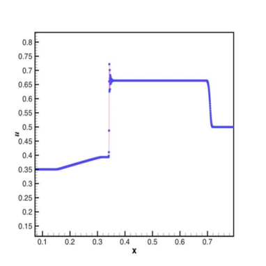
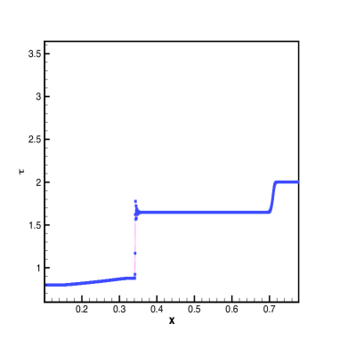
  Figure 19: Typical wave structure for van der Waal fluids; left $u$ and right $\tau$, for $u_{R}=0.5$.

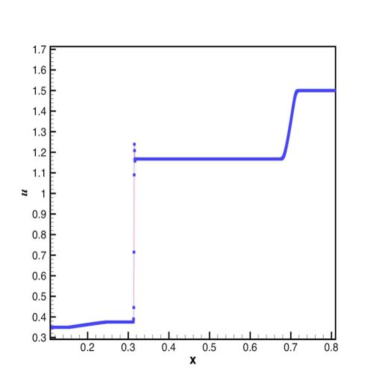
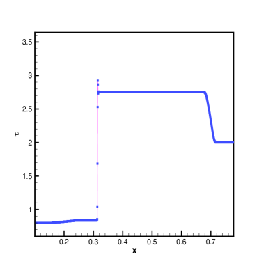
  Figure 20: Typical wave structure for van der Waal fluids; left $u$ and right $\tau$, for $u_{R}=1.5$.

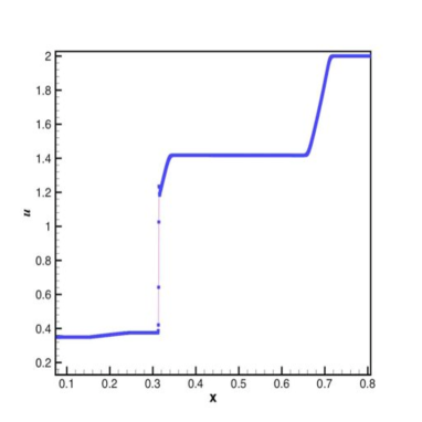
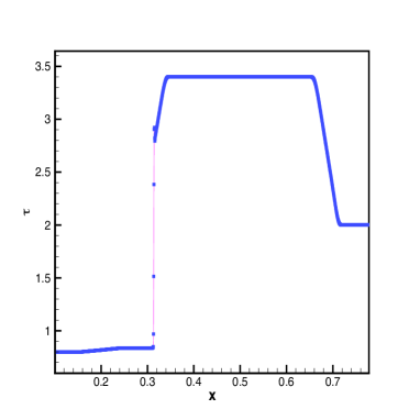
  Figure 21: Typical wave structure for van der Waal fluids; left $u$ and right $\tau$, for $u_{R}=2$.

  

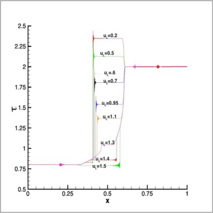
  Figure 22: Wave structure ($\tau$), corresponding to the case $\tau_{L}=0.8$, $\tau_{R}=2$, $u_{R}=1$ and variable $u_{L}$.

  

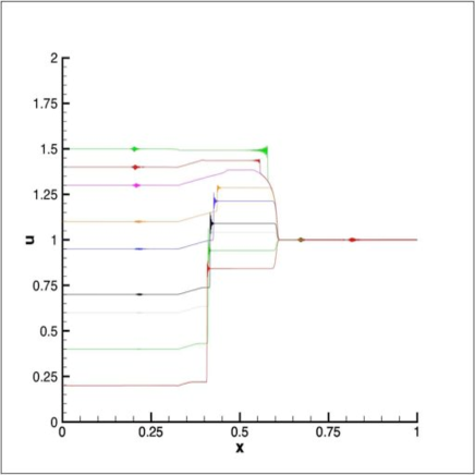
  Figure 23: Wave structure ($u$), corresponding to the case $\tau_{L}=0.8$, $\tau_{R}=2$, $u_{R}=1$ and variable $u_{L}$.

  

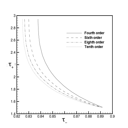
  Figure 24: The kinetic function for $\tau$ obtained for $u_{R}=1$.

  

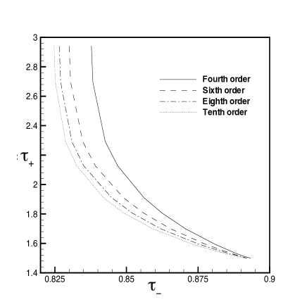
  Figure 25: The kinetic function for $\tau$ obtained for $u_{R}=1.5$.

  

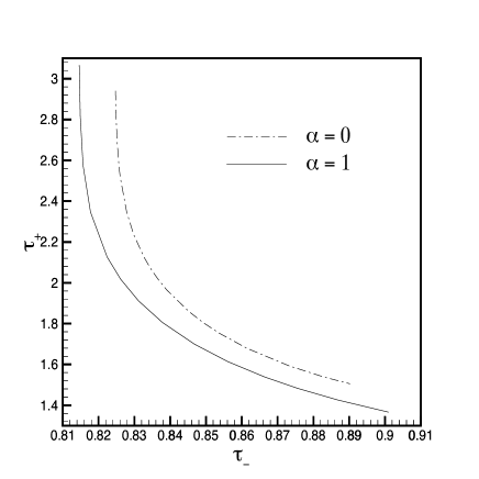
  Figure 26: The kinetic function for $\tau$ obtained for $u_{R}=1$, and capillarity effect with $\alpha=1$, using the tenth order scheme. The dash curve shows the case without the capillarity effect.

  

  Figure 27: A piecewise linear flux function resembling the van der Waals pressure law.

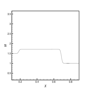
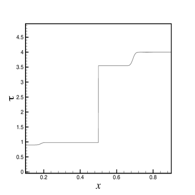
  Figure 28: A typical wave structure in Regime A; $u$ (left) and $\tau$ (right) at time $t=0.12$.

  

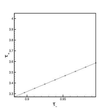
  Figure 29: Kinetic function for Regime A.

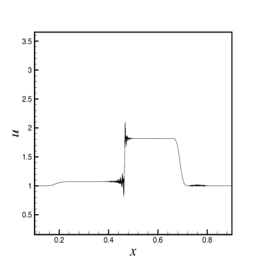
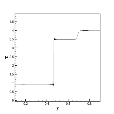
  Figure 30: A typical wave structure in Regime B; $u$ (left) and $\tau$ (right) at time $t=0.12$.

  

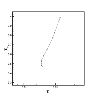
  Figure 31: Kinetic function for Regime B.

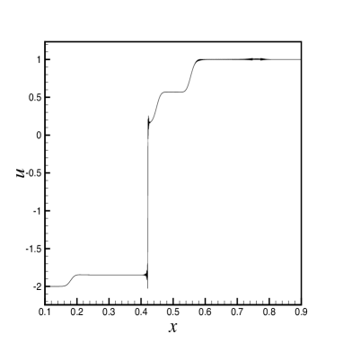
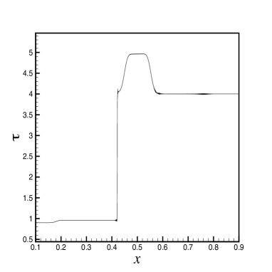
  Figure 32: A typical wave structure in Regime C; $u$ (left) and $\tau$ (right) at time $t=0.12$.

  

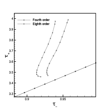
  Figure 33: Kinetic function for both Regims A and B, using the fourth and the eighth order schemes.

6 Concluding remarks

The specific contributions made in this paper are three-fold.

• First, we have investigated the role of the equivalent equation associated with a scheme. We stated a conjecture and provided numerical evidences demonstrating its validity. We have shown that the kinetic function associated with a finite difference scheme approaches the (exact) kinetic function derived from a given (viscosity, capillarity) regularization. Interestingly, the accuracy improves as its equivalent equation coincides with the diffusive-dispersive model at a higher and higher order of approximation. We observed that the spatial accuracy plays a more crucial role than the temporal accuracy. In both the continuous model and the discrete scheme, small scale features are critical to the selection of shocks. Hence, the balance between diffusive and dispersive features determines which shocks are selected. These small scale features can not be quite the same at the continuous and at the discrete levels, since a continuous dynamical system of ordinary differential equations can not be exactly represented by a discrete dynamical system of finite difference equations. The effects of the regularization coefficients on the kinetic functions were also investigated.

• Second, we considered fourth-order models. We demonstrated that a kinetic function can be associated with the thin liquid film model. We also investigated a generalized Camassa-Holm model, and discovered nonclassical shocks for which we could determine a kinetic relation. In both models, the kinetic function was found to be monotone decreasing, as required in the general theory [20].

• Third, we investigated to what extent a kinetic function can be associated with van der Waals fluids, whose flux-function admits two inflection points. We established that the Riemann problem admits several solutions whose discontinuities have viscous-capillary profiles, and we exhibited non-monotone kinetic functions.

In summary, the new features of the kinetic functions observed here suggests directions for further challenging theoretical work on the well-posedness theory for the Cauchy problem associated with nonlinear hyperbolic problems.

Appendix

For completeness we list here the high-order discretizations used in this paper which, for instance, we state for a conservation law with conservative variable $u$ and flux $f=f(u)$.

• Fourth order discretization ($q=4$):

  $$h\,f_{x}={1\over 12}f_{i-2}-{2\over 3}f_{i-1}+{2\over 3}f_{i+1}-{1\over 12}f_{i+2},$$

  $$h^{2}\,u_{xx}=-{1\over 12}u_{i-2}+{4\over 3}u_{i-1}-{5\over 2}u_{i}+{4\over 3}u_{i+1}-{1\over 12}u_{i+2},$$

  $$h^{3}\,u_{xxx}=-{1\over 2}u_{i-2}+u_{i-1}-u_{i+1}+{1\over 2}u_{i+2}.$$

• Sixth order discretization ($q=6$):

  $$h\,f_{x}=-{1\over 60}f_{i-3}+{3\over 20}f_{i-2}-{3\over 4}f_{i-1}+{3\over 4}f_{i+1}-{3\over 20}f_{i+2}+{1\over 60}f_{i+3},$$

  $${h^{2}\over 2}\,u_{xx}={1\over 180}u_{i-3}-{3\over 40}u_{i-2}+{3\over 4}u_{i-1}-{49\over 36}u_{i}+{3\over 4}u_{i+1}-{3\over 40}u_{i+2}+{1\over 180}u_{i+3},$$

  $${h^{3}\over 6}\,u_{xxx}={1\over 48}u_{i-3}-{1\over 6}u_{i-2}+{13\over 48}u_{i-1}-{13\over 48}u_{i+1}+{1\over 6}u_{i+2}-{1\over 48}u_{i+3}.$$

• Eighth order discretization ($q=8$):

  $$\,f_{x}= {1\over 280}f_{i-4}-{4\over 105}f_{i-3}+{1\over 5}f_{i-2}-{4\over 5}f_{i-1}+{4\over 5}f_{i+1}-{1\over 5}f_{i+2}$$

  $$+{4\over 105}f_{i+3}-{1\over 280}f_{i+4},$$

  $${h^{2}\over 2}\,u_{xx}= {-1\over 1120}u_{i-4}+{4\over 315}u_{i-3}-{1\over 10}u_{i-2}+{4\over 5}u_{i-1}-{205\over 144}u_{i}+{4\over 5}u_{i+1}$$

  $$-{1\over 10}u_{i+2}+{4\over 315}u_{i+3}-{1\over 1120}u_{i+4},$$

  $${h^{3}\over 6}\,u_{xxx}= {-7\over 1440}u_{i-4}+{1\over 20}u_{i-3}-{169\over 720}u_{i-2}+{61\over 180}u_{i-1}-{61\over 180}u_{i+1}$$

  $$+{169\over 720}u_{i+2}-{1\over 20}u_{i+3}+{7\over 1440}u_{i+4}.$$

• Tenth order discretization ($q=10$):

  $$h\,f_{x}= {-1\over 1260}f_{i-5}+{5\over 504}f_{i-4}-{5\over 84}f_{i-3}+{5\over 21}f_{i-2}-{5\over 6}f_{i-1}+{5\over 6}f_{i+1}-{5\over 21}f_{i+2}$$

  $$+{5\over 84}f_{i+3}-{5\over 504}f_{i+4}+{1\over 1260}f_{i+5},$$

  $${h^{2}\over 2}\,u_{xx}= {1\over 6300}u_{i-5}-{5\over 2016}u_{i-4}+{5\over 252}u_{i-3}-{5\over 42}u_{i-2}+{5\over 6}u_{i-1}-{5269\over 3600}u_{i}+{5\over 6}u_{i+1}$$

  $$-{5\over 42}u_{i+2}+{5\over 252}u_{i+3}-{5\over 2016}u_{i+4}+{1\over 6300}u_{i+5},$$

  $${h^{3}\over 6}\,u_{xxx}= {41\over 36288}u_{i-5}-{1261\over 90720}u_{i-4}+{541\over 6720}u_{i-3}-{4369\over 15120}u_{i-2}+{1669\over 4320}u_{i-1}$$

  $$-{1669\over 4320}u_{i+1}+{4369\over 15120}u_{i+2}-{541\over 6720}u_{i+3}+{1261\over 90720}u_{i+4}-{41\over 36288}u_{i+5}.$$

References

- [1] R. Abeyaratne and J.K. Knowles, Kinetic relations and the propagation of phase boundaries in solids, Arch. Ration. Mech. Anal. 114 (1991), 119–154.
- [2] R. Abeyaratne and J.K. Knowles, Implications of viscosity and strain-gradient effects for the kinetics of propagating phase boundaries in solids, SIAM J. Appl. Math. 51 (1991), 1205–1221.
- [3] N. Bedjaoui, C. Chalons, F. Coquel, and P.G. LeFloch, Non-monotonic traveling waves in Van der Waals fluids, Analysis Appl. 3 (2005), 419–446.
- [4] N. Bedjaoui, C. Klingenberg, and P.G. LeFloch, On the validity of the Chapman-Enskog expansion for shock waves with small strength, Portugal. Math. 61 (2004). 479–499.
- [5] N. Bedjaoui and P.G. LeFloch, Diffusive-dispersive traveling waves and kinetic relations V. Singular diffusion and nonlinear dispersion, Proc. Royal Soc. Edinburgh 134A (2004), 815–843.
- [6] A.M. Bertozzi, A. Münch, and M. Shearer, Undercompressive shocks in thin film flows, Phys. D 134 (1999), 431–464.
- [7] A.L. Bertozzi and M. Shearer, Existence of under-compressive traveling waves in thin film equations, SIAM J. Math. Anal. 32 (2000), 194–213.
- [8] C. Chalons and P.G. LeFloch, High-order entropy conservative schemes and kinetic relations for van der Waals fluids, J. Comput. Phys. 167 (2001), 1–23.
- [9] C. Chalons and P.G. LeFloch, Computing under-compressive waves with the random choice scheme. Non-classical shock waves, Interfaces Free Bound. 5 (2003), 129–158.
- [10] R.M. Colombo and A. Corli, Sonic and kinetic phase transitions with applications to Chapman-Jouguet deflagration, Math. Methods Appl. Sci. 27 (2004), 843–864.
- [11] A. Corli and H.T. Fan, The Riemann problem for reversible reactive flows with metastability, SIAM J. Appl. Math. 65 (2004), 426–457.
- [12] H.T. Fan and H.-L. Liu, Pattern formation, wave propagation and stability in conservation laws with slow diffusion and fast reaction, J. Hyperbolic Differ. Equ. 1 (2004), 605–636.
- [13] H.-T. Fan and M. Slemrod, The Riemann problem for systems of conservation laws of mixed type, in “Shock induced transitions and phase structures in general media”, Workshop held in Minneapolis (USA), Oct. 1990, Dunn J.E. (ed.) et al., IMA Vol. Math. Appl. 52 (1993), pp. 61-91.
- [14] B.T. Hayes and P.G. LeFloch, Nonclassical shocks and kinetic relations. Scalar conservation laws, Arch. Ration. Mech. Anal. 139 (1997), 1–56.
- [15] B.T. Hayes and P.G. LeFloch, Nonclassical shocks and kinetic relations. Finite difference schemes, SIAM J. Numer. Anal. 35 (1998), 2169–2194.
- [16] B.T. Hayes and P.G. LeFloch, Nonclassical shock waves and kinetic relations. Strictly hyperbolic systems, SIAM J. Math. Anal. 31 (2000), 941–991.
- [17] T.Y. Hou and P.G. LeFloch Why nonconservative schemes converge to wrong solutions: error analysis, Math. Comp. 62 (1994), 497–530.
- [18] D. Jacobs, W.R. McKinney, and M. Shearer, Traveling wave solutions of the modified Korteweg-deVries Burgers equation, J. Differential Equations 116 (1995), 448–467.
- [19] P.G. LeFloch, Propagating phase boundaries: formulation of the problem and existence via the Glimm scheme, Arch. Ration. Mech. Anal. 123 (1993), 153–197.
- [20] P.G. LeFloch, Hyperbolic systems of conservation laws: The theory of classical and non-classical shock waves, Lectures in Mathematics, ETH Zürich, Birkäuser, 2002.
- [21] P.G. LeFloch, Graph solutions of nonlinear hyperbolic systems, J. Hyperbolic Differ. Equ. 1 (2004), 643–690.
- [22] P.G. LeFloch and C. Rohde, High-order schemes, entropy inequalities, and non-classical shocks, SIAM J. Numer. Anal. 37 (2000), 2023–2060.
- [23] P.G. LeFloch and M. Shearer, Nonclassical Riemann solvers with nucleation, Proc. Roy. Soc. Edinburgh Sect. A 134 (2004), 941–964.
- [24] R. Levy and M. Shearer, Comparison of dynamic contact line models for driven thin liquid films, Euro. J. Applied Math. 15 (2004), 625–642.
- [25] A. Münch, Shock transitions in Marangoni gravity driven thin film flow, Nonlinearity 13 (2000), 731–746.
- [26] S.-C. Ngan and L. Truskinovsky, Thermo-elastic aspects of dynamic nucleation, J. Mech. Phys. Solids 50 (2002), 1193–1229.
- [27] F. Otto and M. Westdickenberg, Convergence of thin film approximation for a scalar conservation law, J. Hyperbolic Differ. Equ. 2 (2005), 183–200.
- [28] S. Schulze and M. Shearer, Undercompressive shocks for a system of hyperbolic conservation laws with cubic nonlinearity, J. Math. Anal. Appl. 229 (1999), 344–362.
- [29] M. Slemrod, Admissibility criteria for propagating phase boundaries in a van der Waals fluid, Arch. Ration. Mech. Anal. 81 (1983), 301–315.
- [30] M. Slemrod, A limiting viscosity approach to the Riemann problem for materials exhibiting change of phase, Arch. Ration. Mech. Anal. 105 (1989), 327–365.
- [31] L. Truskinovsky, Dynamics of non-equilibrium phase boundaries in a heat conducting nonlinear elastic medium, J. Appl. Math. and Mech. (PMM) 51 (1987), 777–784.
- [32] L. Truskinovsky, Kinks versus shocks, in “Shock induced transitions and phase structures in general media”, R. Fosdick, E. Dunn, and M. Slemrod ed., IMA Vol. Math. Appl., Vol. 52, Springer-Verlag, New York (1993), pp. 185–229.
- [33] C. Tsitouras and S.N. Papakostas, Cheap error estimation for Runge-Kutta methods, SIAM J. Sci. Comput. 20 (1999), 2067–2088.
- [34] C. Tsitouras, Optimized explicit Runge-Kutta pair of order 9, Appl. Numer. Math. 38 (2001) 123–134.