Spitzer 24µm Time-Series Observations of the Eclipsing M-dwarf Binary GU Boötis

Abstract

We present a set of Spitzer 24$\mu$m MIPS time series observations of the M-dwarf eclipsing binary star GU Boötis. Our data cover three secondary eclipses of the system: two consecutive events and an additional eclipse six weeks later. The study’s main purpose is the long wavelength (and thus limb darkening-independent) characterization of GU Boo’s light curve, allowing for independent verification of the results of previous optical studies. Our results confirm previously obtained system parameters. We further compare GU Boo’s measured 24$\mu$m flux density to the value predicted by spectral fitting and find no evidence for circumstellar dust. In addition to GU Boo, we characterize (and show examples of) light curves of other objects in the field of view. Analysis of these light curves serves to characterize the photometric stability and repeatability of Spitzer’s MIPS 24µm array over short (days) and long (weeks) timescales at flux densities between approximately 300–2,000$\mu$Jy. We find that the light curve root mean square about the median level falls into the 1–4% range for flux densities higher than 1mJy. Finally, we comment on the fluctuations of the 24µm background on short and long timescales.

1. Introduction

GU Boötis is a nearby, low-mass eclipsing binary system, consisting of two nearly equal mass M-dwarfs (López-Morales & Ribas, 2005). It is one of currently very few ($\sim$5) known nearby ($<$ 200 pc) double-lined, detached eclipsing binary (DEB) systems composed of two low-mass stars (López-Morales, 2007). Eclipsing binaries can be used as tools to constrain fundamental stellar properties such as mass, radius, and effective temperature. Given the fact that over 70% of the stars in the Milky Way are low-mass objects with $M<1M_{\odot}$ (Henry et al., 1997), coupled with the considerable uncertainty over the mass-radius relation for low-mass stars, objects such as GU Boo are of particular interest in exploring the low-mass end of the Hertzsprung-Russell diagram.

While simultaneous analysis of DEB light curves and radial velocity (RV) curves provides insight into the component masses and physical sizes, an estimate of their intrinsic luminosities can only be made with the knowledge of the amount and properties of dust along the line of sight. As such, it is important to understand whether low-mass DEB systems used to constrain stellar models contain dust which, in turn, may lead to an underestimate of their surface temperatures and thus luminosities. This problem has been documented in Delfosse et al. (1999); Mazeh et al. (2001); Torres & Ribas (2002); Ribas (2003). In particular, Ribas (2003) states that the most likely explanation for the temperature discrepancy between observations and models for the low-mass DEB CU Cancri is the presence of either circumstellar or circumbinary dust. The detection of dust in any system such as GU Boo would therefore additionally shed insight into formation and evolution of the low-mass DEBs.

The characterization of the effects of limb darkening and star spots introduces additional free parameters and thus statistical uncertainty in the calculation of the stellar radii and masses. Using the Spitzer Space Telescope, we obtained 24$\mu$m time series observations of three separate instances of GU Boo’s secondary eclipse (see §2.1) to create a light curve far enough in the infrared to not be contaminated by the effects of limb darkening and star spots. We purposely timed the observations such that each secondary eclipse event is preceded by a sufficient length of time to establish GU Boo’s out-of-eclipse flux density in order to detect any infrared excess possibly caused by thermal dust emission.

A further goal of our study is to characterize the photometric stability of the Multiband Imaging Photometer (MIPS) on Spitzer at 24$\mu$m over short and long time scales, similar to what was done for bright objects in §5 of Rieke et al. (2004). Time-series observing is atypical (albeit increasingly common) for Spitzer, which is the reason why there are very few published photometric light curves based on Spitzer observations. The recent spectacular observations of primary and secondary eclipses of transiting planets are notable exceptions (see for instance Charbonneau et al., 2005; Deming et al., 2005; Cowan et al., 2007; Deming et al., 2007; Gillon et al., 2007; Knutson et al., 2007). Of these, the Deming et al. (2005) study was performed at 24$\mu$m. We therefore observed two consecutive secondary eclipses of GU Boo ($\sim$ 12 hours apart), and then a third event about six weeks later (see Table 1).

We describe our observations and data reduction methods in §2 and discuss our findings with respect to Spitzer’s photometric stability in §3. The analysis of GU Boo’s light curve is described in §4. We probe for the existence of an infrared excess in GU Boo’s spectral energy distribution in §5. In §6, we show light curves of other well sampled objects in the field along with a brief summary of their respective properties, and we summarize and conclude in §7.

2. Spitzer Observations and Data Reduction

2.1. Observations

We used the MIPS 24µm array aboard the Spitzer Space Telescope (Werner et al., 2004) to observe GU Boo in February and April of 2006, as outlined in Table 1. The MIPS 24µm array (MIPS-24), is a Si:As detector with 128 $\times$ 128 pixels, an image scale of 2.55” pixel^-1, and a field of view of 5.4’ $\times$ 5.4’ (Rieke et al., 2004). Our exposures were obtained using the standard MIPS 24$\mu$m small field photometry pattern, which consists of four cardinal dither positions located approximately in a square with 2 arcmin on a side. For two of these cardinal positions, there are four smaller subposition dithers (offset by $\sim$ 10 arcsec), and for the other two cardinal positions, there are three such subpositions. This results in a dither pattern in which Spitzer places the star at 14 different positions on the array.

Our goal was to observe three independent secondary eclipses of GU Boo: two consecutive ones and another one several weeks after the first two (von Braun et al., 2007). Of our total of nine of Spitzer’s Astronomical Observation Requests (AORs), three were used for each secondary eclipse event (see Table 1). Each AOR contained eight exposures with 36 individual Basic Calibrated Data (BCD) frames each. The first BCD in each exposure is 9s long, the subsequent 35 are 10s long. The first two BCDs of every exposure were discarded due to a “first frames effect”. This procedure left 34 BCDs per exposure, 272 BCDs per AOR, 816 BCDs per secondary eclipse event, and 2448 BCDs for the entire project (all 10s exposure time).

For background information on Spitzer and MIPS, we refer the reader to the Spitzer Observer’s Manual, obtainable at http://ssc.spitzer.caltech.edu/documents/som/. For information specifically related to MIPS data reduction, please consult the MIPS Data Handbook (MDH – http://ssc.spitzer.caltech.edu/mips/dh/) and Gordon et al. (2005).

Table 1Spitzer MIPS-24 observations of GU Boötis

Date (2006)	MIPS Campaign	Obs. Set	AORs	Exposures
Feb 20	MIPS006500	1	16105472	860
			16105216
			16104960
Feb 21	MIPS006500	2	16104704	860
			16104448
			16104192
Apr 01	MIPS006700	3	16103936	860
			16103680
			16103424

Note. — Two consecutive secondary eclipses were observed in observing sets 1 and 2, and a third secondary eclipse event six weeks later in observing set 3.

2.2. Data Processing and mopex $/$ apex Reduction

2.2.1 Mosaicing

The MIPS-24 data are provided by the Spitzer Archive in the (flatfielded) BCD format. We applied further post-processing to these data in order to correct for small scale artifacts, in particular using IRAF’s CCDRED package to remove the weak “jailbar” features in the images (as described in the MDH).

The Spitzer software package mopex (Makovoz & Khan, 2005; Makovoz & Marleau, 2005) was used to co-add the individual MIPS BCD frames into mosaics of 17 frames, using overlap correction and outlier rejection in the process. The choice of 17 frames was made to balance three aspects:

1. We want to obtain sufficient signal-to-noise ratio (SNR) for measured flux densities in the combined images and subsequent data points in the light curves (SNR $>$ 10 for GU Boo; see Table 3).

2. We need to maintain a sufficiently high effective observing cadence to temporally resolve elements of GU Boo’s light curve for fitting purposes.

3. We do not want to be forced to combine frames from different exposures into a single light curve data point (see §2.1).

The interpolated, remapped mosaics have a pixel scale of 2.45” pixel^-1. We show in Figure 1 the MIPS-24 field of view of GU Boo.

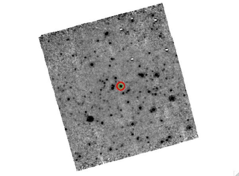
Figure 1.— A Spitzer MIPS 24$\mu$m mosaic of GU Boo (marked with a circle at the center of the image). This mosaic was created using all 272 frames in one AOR and is about 8 arcmin on a side. North is up, east is to the left. The change in noise structure as a function of position is due to different effective exposure times (only the inner $\sim$ 3’ $\times$ 3’ were covered by all 272 BCD frames). The white specks in the NW corner are flatfielding residuals, caused by a fleck of paint or dust grain on the pickoff mirror (from Spitzer’s launch), imaged at the four cardinal dither positions (see §2.1).

2.2.2 Photometry

For photometric reductions of the mosaiced images, we utilized the apex component of mopex to perform point-source extraction as described in Makovoz & Marleau (2005). This step included background subtraction of the images, and the fitting of a resampled point response function (PRF). In order to match the PRF centroid as closely as possible to the centroid of the stellar profile, the first Airy ring is initially subtracted from the stellar profiles, and the source detection happens on the resulting image. Photometry of the detected sources is then performed on the original images.

For single frame photometry on mosaiced images, apex provides the option of using a template model PRF produced by the analysis of $\sim$ 20 bright, isolated stars in the Spitzer Archive, or using one’s own data to create a PRF. It furthermore allows for a resampling factor in both x and y directions. The scatter in our light curves was minimized when using the model PRF provided by the Spitzer Science Center, oversampled by a factor of 4 in both x and y directions. Using the PRF created from our own data or sampling any PRF to a higher resolution resulted in noticeably larger root mean square (rms) dispersion in our light curves, most likely due to systematic errors introduced in the low SNR regime of our data (see Table 3).

We note that, currently, apex only provides the option of using a synthetic PRF (Tiny Tim; Krist, 1993) for photometry on individual BCD frames (i.e., not mosaiced), as applied by Deming et al. (2005) and Richardson et al. (2006). Since the flux density of our target star ($\sim$ 600$\mu$Jy) is so much lower than HD 209458 ($\sim$22mJy; Deming et al., 2005), our SNR regime did not allow for performing photometry on single BCD frames.

2.2.3 Background Fluctuations

The apex error analysis is described in the apex User’s Guide, and parts of it can be found in Makovoz et al. (2002); Makovoz & Lowrance (2005); Makovoz & Marleau (2005). We briefly summarize the general idea here. Errors in the photometry are dominated by the statistical background fluctuations in the images. These fluctuations are calculated per pixel by estimating the Gaussian noise inside a sliding window whose size is defined by the user (45 $\times$ 45 interpolated pixels in this case). Thus, apex produces “noise tiles” for the computation of the SNR of the point sources in the corresponding mosaiced image tiles (see column 7 in Table 3).

To provide an estimate of the background fluctuations from image to image, we show in Fig. 2 the surface brightness for every image in the three observing sets. These estimates were obtained by calculating the median surface brightness level for the inner 90% of the image (in area). The error bars correspond to the standard deviation about this median over the same area. Note that the fluctuations of the background within observing sets are very small, but they are different for the temporally offset observing set 3 (see Table 1). Surface brightness values are given in the Spitzer native units of MJy per steradian. The surface brightness values in the cores of the brightest objects in the field are typically 1–1.5 MJy/sr above the background level (23–25 MJy/sr). A linear fit (weighted by the standard deviation values of the data points) to observing sets 1 & 2 returns a slope of $-0.033\pm 0.023$ MJy/sr/day. The same fit for all three observing sets produced a statistically consistent slope of $-0.030\pm 0.001$ MJy/sr/day, indicating a smoothly decreasing background level over the course of our observations (Table 1).

The Spitzer tool Spot predicts the surface brightness of the Zodiacal background in Spitzer images. Harrington et al. (2006), for instance, used this model to correct for ostensible variations in instrument sensitivity over a period of around four days. We compared our background estimates to the predictions in Spot and found that the model underestimates our measurements by 3.5–4.0 MJy/sr. One potential reason for any offset between observed and estimated backgrounds is that Spot calculates a monochromatic background, whereas the measured background is integrated over the wavelength passband and sensitivity function of the MIPS-24 detector. Using Spot, we calculated background estimates in 6 hour increments from 2006 Feb 20 00:00:00 to 2006 Feb 22 00:00:00, and from 2006 Apr 01 00:00:00 to 2006 Apr 02 00:00:00. The slopes of the Feb backgrounds and the Feb–Apr backgrounds are -0.022 and -0.032 MJy/sr/day, respectively; Spot does not provide error estimates in its predictions. It thus appears that, within statistical uncertainties, the behavior of the Spot background model is consistent with our empirical results (at least for the time scales of our observations), lending further justification to the approach by Harrington et al. (2006).

If, however, the difference in slope between the Spot estimates for just Feb and Feb–Apr is indeed real but simply not detectable at our temporal resolution (indicating that the background change with time is not a simple linear function), any resulting discrepancy between calculated and observed background values may be attributable to the fact that the model is calculated for Earth, whereas Spitzer is in an Earth-trailing orbit and thus looking through different amounts of Zodiacal dust (Harrington et al., 2006).

Figure 2.— Temporal fluctuations of the image background measured in surface brightness units of MJy/sr for the three observing sets (1). The lower, middle, and upper panel correspond to observing set 1, 2, and 3, respectively. Note that the background level is similar between observing sets 1 and 2 ($24.48\pm 0.009$ MJy/sr and $24.46\pm 0.009$ MJy/sr, respectively), but lower for observing set 3 ($23.28\pm 0.008$ MJy/sr). The typical fluctuations within a given image (represented by the error bars) are around 0.05–0.06 MJy/sr. The large error bar for the one data point in observing set 3 is caused by a cosmic ray.

3. Precision and Repeatability of the Spitzer Photometry

3.1. PRF Fitting Versus Aperture Photometry

To create GU Boo’s 24µm light curve, we performed both PRF photometry as described in §2.2 and additionally utilized apex’s option of simultaneously obtaining aperture photometry. Figure 3 shows the agreement between PRF and aperture photometry based on an aperture radius of 6” (with 20–32” background annulus) which minimized the rms in the flat part of GU Boo’s phased light curve. Using information from the MDH, we applied a multiplicative aperture correction of 1.699 to the photometry. The median flux density obtained by PRF photometry for the flat part of the phased light curve is 614 $\pm$ 49$\mu$Jy compared to 608 $\pm$ 59$\mu$Jy for the aperture photometry. Thus, the absolute median flux density values agree very well for the two different photometry approaches, but the PRF photometry exhibits smaller scatter around the median magnitude. We note that the current version of apex does not calculate photometry errors in the aperture correction, and the principal reason why we performed aperture correction is to verify the absolute flux density level of our sources as calculated by PRF fitting.

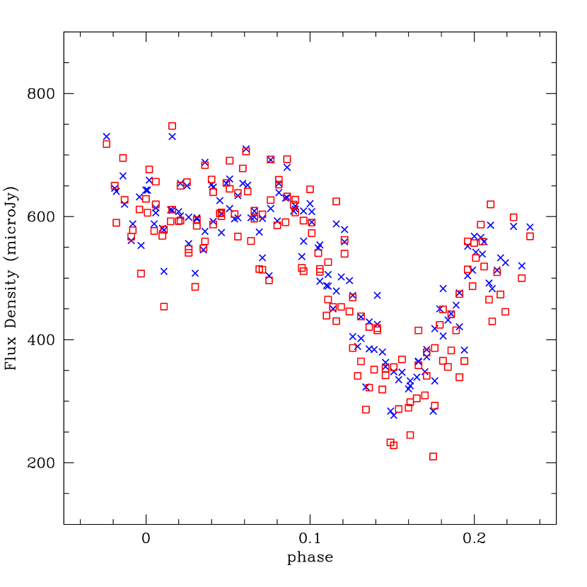
Figure 3.— Comparison between PRF photometry (blue crosses) and aperture photometry (red squares) for GU Boo’s phased light curve. Photometric error bars are omitted for the sake of clarity. The scatter in the flat part of the light curve is smaller for PRF photometry (49$\mu$Jy) than aperture photometry (59$\mu$Jy), but the median flux density level of the flat part of the light curve is identical within the errors for both photometry approaches.

3.2. Absolute Versus Relative Photometry

In order to remove statistically correlated noise from GU Boo’s light curve, we performed relative photometry as described in equations 2 and 3 of Everett & Howell (2001). We picked comparison objects based on the number of observational epochs: in order to obtain a relative offset per photometric data point in GU Boo’s light curve (all data points are treated independently of each other), it is advantageous to use stars with (at least) as many data points as GU Boo itself. Four objects out of Table 3 fulfill this criterion: numbers 18, 31, 58, and 66 (see Figures 10–12 for their light curves). The cross-referencing in Table 3 shows that objects 31 and 66 are stars, and objects 18 and 58 are galaxies (as are all other objects in the field that we were able to cross-reference). Note, however, that object 31’s closest match in SDSS (Adelman-McCarthy & et al., 2007) and 2MASS (Cutri et al., 2003a; Skrutskie et al., 2006) catalogs is 9” away whereas for object 66, the distance to the closest SDSS match was only 0.15”. We originally presumed that, despite the fact that they are galaxies, objects 18 and 58 would be unresolved at our large pixel size (§2.1) and tested that hypothesis by comparing the flux density obtained by PRF photometry to that obtained by aperture photometry (6” aperture; §3.1). Figures 4 and 5 shows that our presumption does not hold true for object 58, and we discarded it from our relative photometry procedure.

We find that, by performing differential photometry as outlined above, the scatter in the flat part of GU Boo’s phased light curve reduces by 9.4% over the PRF photometry (see Fig. 3) to 45$\mu$Jy. Light curve fitting as described in §4 was performed on the differential photometry.

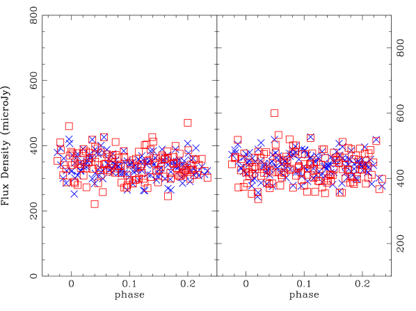
Figure 4.— Comparison between PRF photometry (blue crosses) and aperture photometry (red squares) for objects 31 (left) and 66 (right). Photometric error bars are omitted for the sake of clarity. The light curves are phased to the period of GU Boo for the sake of comparison. The ordinate scale is the same as Figures 3, 5, and 10–12. The flux density values (PRF vs aperture photometry) are identical within the errors for both objects.

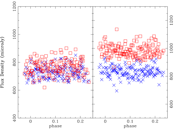
Figure 5.— Comparison between PRF photometry (blue crosses) and aperture photometry (red squares) for objects 18 (left) and 58 (right). Photometric error bars are omitted for the sake of clarity. The light curves are phased to the period of GU Boo for the sake of comparison. The ordinate scale is the same as Figures 3, 4, and 10–12. The flux density values (PRF vs aperture photometry) agree within the errors for object 18, but are discrepant for object 58.

3.3. Intra-Set Versus Inter-Set Photometric Stability

Figure 6 shows fractional rms values versus median flux densities for all objects in Table 3. For every object, we plot fractional rms for each individual observing set as well as for the three sets combined. Observing sets 1 and 2 were obtained during the MIPS006500 campaign, observing set 3 during MIPS006700 (Table 1). Consistent with the results in Rieke et al. (2004), we find that inter-set repeatability of Spitzer’s MIPS-24 is comparable to the intra-set repeatability, both in terms of median flux density and the rms scatter of the light curves, despite varying background levels (see §2.2.3). For objects with a flux density in excess of 1mJy, the rms scatter approaches 1–2 %, similar to the scatter found for the brightest sources observed with MIPS-24 in Rieke et al. (2004). Because of the intrinsic variability produced by the stellar eclipse, GU Boo has the largest fractional rms ($\sim$ 0.2). However, when we subtract the fit (see §4) from GU Boo’s light curve, the fractional rms falls to 0.081, consistent with stars of similar median brightness. We show GU Boo’s light curve for the three individual observing sets in Fig. 7 and the phased light curve along with the fit in Fig. 8.

In order to compare our rms values to background-limited noise values, we used Spitzer’s SENS-PET to predict the MIPS-24 sensitivity ($1\sigma$ above background for 170 seconds integration time; see §2.2.1) for low and medium background levels (solid and dashed line in Fig. 6, respectively). The mid-infrared background at the time of observations of GU Boo is 23–24.5 MJy/sr, which is between the typical low and medium background levels used by SENS-PET (see also §2.2.3). We find that the SENS-PET predictions are consistent with our empirically determined error estimates. Except for the variable GU Boo, typical values for the rms scatter of the light curves (Table 3) are approximately equal to average photometric measurement uncertainties of individual data points (see Figs. 10, 11, and 12).

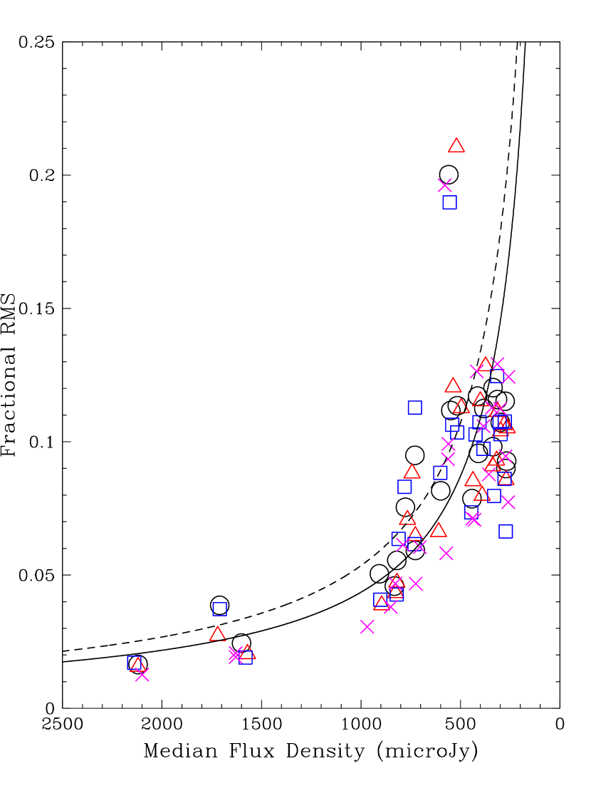
Figure 6.— Median flux density versus fractional rms for the 24 objects that have photometry for more than 72 out of 144 observational epochs. Triangles, squares, and crosses represent the data from observings sets 1, 2, and 3, respectively (see Table 1), to illustrate the repeatability of Spitzer/MIPS-24 within individual observing sets. Circles mark the data points from the combination of all 3 observing sets (to show the inter-set stability). The data point with the highest fractional rms is GU Boo, due to its intrinsic variability. When subtracting our fit from its light curve (see Fig. 8), GU Boo’s fractional rms falls to 0.081. The solid and dashed lines indicate MIPS-24’s sensitivity for our exposure times as a function of flux density for low and medium background levels, respectively.

Figure 7.— GU Boo’s 24$\micron$ light curve, based on absolute PRF photometry (see §3.1 and §3.2). The three panels represent the three MIPS-24 observing sets during which the individual secondary eclipse events were observed. GU Boo is object number 51 in our numbering system (see Table 3).

4. Analysis of GU Boo’s Photometric Light Curve

We modeled the secondary eclipse observations of GU Boo using the JKTEBOP code (Southworth et al., 2004a, b). JKTEBOP is based on the original EBOP code (Popper & Etzel, 1981; Etzel, 1981), but with the addition of the Levenberg-Marquardt optimization algorithm (Press et al., 1992) to find the best fitting model, and also the implementation of a Monte Carlo simulation algorithm to determine robust uncertainties in the fitted parameters (Southworth et al., 2005).

The orbital period and initial epoch of the primary eclipse were set to the values given in the ephemeris derived by López-Morales & Ribas (2005). We further fixed the mass ratio and the radius ratio of the stars, as well as the eccentricity of the system ($e$=0) to the values obtained in that work. We assumed no limb darkening effects in the light curves, as expected for observations this far into the infrared (Claret et al., 1995; Richardson et al., 2006; Ciardi et al., 2007; Snellen, 2007, and references therein), and no significant gravitational darkening or reflection effects, based on the spherical shape of the stars and the similarity in effective temperatures. All these are reasonable assumptions, based on the results of the study of GU Boo at visible wavelengths, and they are, in fact, hard to test in detail, given the photometric precision of the Spitzer light curve at this flux density level.

In the absence of primary eclipse observations, to calculate the luminosity ratio of the system, we place a further constraint to the fit by fixing the value of the surface brightness ratio of the stars to J=J2/J1=0.9795. This value, combined with the adopted radius ratio and the no limb darkening assumption, gives a luminosity ratio of of $L_{2}/L_{1}$ = 0.9697, which is consistent with the expected value for GU Boo at 24$\mu$m.

The parameters initially left free in the models were: (1) the fractional sum of the radii, i. e., $(R_{1}+R_{2})/a$, where $R_{1}$ and $R_{2}$ are the component radii, and $a$ is the orbital separation, computed from the stellar masses and the orbital period of the system, (2) the inclination of the orbit $i$, (3) the amount of third light $L_{3}$, and (4) a phase offset parameter $\phi$ (to account for small errors in the ephemeris).

Our best model solution is illustrated in Figure 8, with a reduced $\chi^{2}$ of 1.7, and a mean fractional error per data point of 9.5% (cf. Fig. 6). Formal errors in the fitted parameters were derived using the Monte Carlo algorithm implementation in JKTEBOP for a total of 1000 iterations. We obtain a radius for the secondary component of $R_{2}$ = 0.66 $\pm$ 0.02 $R_{\sun}$. Our value of the orbital inclination is $i$ = 89.3 $\pm$ 0.8 degrees. Both values are slightly larger than the ones obtained by López-Morales & Ribas (2005) at optical wavelengths, $R_{2}$ = 0.62 $\pm$ 0.02 $R_{\sun}$ and $i$ = 87.6 $\pm$ 0.2 degrees. The two secondary radius estimates agree to within random statistical errors (1.4$\sigma$). In the case of the inclination, our value is not as well constrained as in the optical, since we lack a full light curve that includes a primary eclipse. We show our estimates for GU Boo’s system parameters in Table 2. For the tested third light contribution, we obtain a value of $L_{3}$ = -0.04 $\pm$ 0.07, consistent with $L_{3}$ = 0.

Finally, we find a phase shift of $\Delta\phi$ = -0.014 $\pm$ 0.001. This phase shift is 1.5 times larger than expected from the López-Morales & Ribas (2005) ($|\Delta\phi|$ = 0.009), but can still be attributed to uncertainties in the original period estimation. The López-Morales & Ribas (2005) observations were conducted in 2003, near JD=2452733. The number of elapsed periods inbetween those observations and our Spitzer AORs is about 2150. The 1-$\sigma$ error in the López-Morales & Ribas (2005) period estimate is $2\times 10^{-6}$ days, which accumulates to 0.0043 days, about 0.009 in phase, in 2150 periods. Thus, the discrepancy we find corresponds to about 1.5$\sigma$ from the López-Morales & Ribas (2005) ephemeris predictions. We estimate that this offset is based on normal statistiscal errors. An alternative explanation would be that a third body orbiting the system could cause this shift, but since (1) we show in §5 that GU Boo’s flux is consistent with its modeled spectral energy distribution, and (2) we calculate the third light component to be $L_{3}$ = 0, any such claim would be unsubstantiable with our data.

Equation 1 shows the updated ephemeris equation of GU Boo by combining the seven minima in table 5 of López-Morales & Ribas (2005) with the three new minima presented in this work.

$$T(\mbox{Min I})=\mbox{HJD}2452723.981327(1)+0.4887247(8)\cdot E.$$ (1)

Uncertainty digits are given in parentheses. $E$ represents the number of elapsed periods since the initial epoch, $T(\mbox{Min I})$ the time of primary eclipse minimum.

Table 2GU Boo System Parameters

Parameter	Value
Orbital Period (days)	$0.488728\pm 0.000002$
Orbital Eccentricity	0 (fixed)
Mass Ratio (M2/M1)	$0.9832\pm 0.0069$
Combined out-of-eclipse 24 µm flux ($\mu$Jy)	$614\pm 49$
Radius of Secondary Component ($R_{\sun}$)	0.66 $\pm$ 0.02 (0.62)
Orbital Inclination $i$ (degrees)	89.3 $\pm$ 0.8 (87.6)

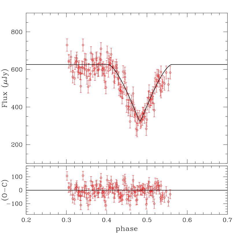
Figure 8.— Our best fit overlaid on top of the phased 24$\micron$ data of GU Boo derived from our relative photometry of the system. The fit has a reduced $\chi^{2}=1.7\pm$ 0.1. The bottom panel shows the residuals around the fit. The calculated system parameters, which agree well with the results from the optical study in López-Morales & Ribas (2005), are shown in Table 2.

5. Comparison Between Expected and Measured 24µm Flux Density of GU Boo

In addition to the relative photometry of GU Boo (Fig. 8), we also performed absolute photometry as reported in §3.1. The 24µm flux density of $614\pm 49\mu$Jy was determined from the median flux level outside of eclipse. To test the accuracy of the absolute flux density level, we show in this section a spectral energy distribution (SED) model between 0.11 and 35$\micron$, scaled to the optical and near-infrared (NIR) magnitudes of GU Boo (López-Morales & Ribas, 2005).

The GU Boo system components are two M stars of nearly identical mass, temperature and radius. For our SED model, we assumed both stellar components to be M1V stars with effective temperatures of 3800 K (e.g., López-Morales & Ribas, 2005). The model SED was constructed from the M1V $0.11-2.5$µm optical-NIR templates of Pickles (1998) and the Spitzer $5-35$µm Infrared Spectrograph (IRS; Houck et al., 2004) spectra of GL 229A, an M1V (3800 K) star (Cushing et al., 2006). To build the SED model (Fig. 9), the M1V optical-NIR template was scaled to GU Boo’s optical-NIR flux densities based on table 1 in López-Morales & Ribas (2005). To connect the Spitzer IRS spectrum to the optical-NIR template, we fit a power law of the form $F_{\nu}\propto\nu^{n}$ (see dashed line in Fig. 9) to the IRS spectrum. We found the best-fit exponent to the power law to be $n=1.9$. The IRS spectrum and the power law (extrapolated to 2.4$\micron$) were then scaled to the red edge of the optical-NIR template. The slope of the power law was maintained to ensure a continuous transition between the optical-NIR template and the IRS spectrum (see Fig. 9). Note that only the optical and NIR flux densities were used to scale the SED model; i.e., the scaling does not utilize the 24µm data point.

The SED model predicts a mid-infrared flux density for GU Boo of $F_{\nu}(24\mu{\rm m})\approx 650\mu$Jy. The measured 24µm flux density of GU Boo ($614\pm 49\mu$Jy) is within 1$\sigma$ of the predicted flux density, agreeing remarkably well with the simple SED model presented here. We conclude that the stellar components are solely responsible for the mid-infrared emission of GU Boo.

The few M- and K-dwarf DEB systems studied to date (GU Boo included) reveal that many of the binary components have larger radii (by 10-20%) and cooler effective temperatures (by 100 K to hundreds of K) than predicted by stellar evolutionary models (e.g., Torres & Ribas, 2002; Ribas, 2003; López-Morales & Ribas, 2005; López-Morales, 2007). Magnetic activity and metallicity can account for the radius discrepancy (López-Morales, 2007) and, in principle, also for the temperature discrepancy. An alternative explanation for the temperature discrepancy, however, is the presence of dusty material around the systems. The excellent agreement of our observed mid-infrared flux density with the model SED suggests that there is little, if any, (warm) circumstellar dust in GU Boo, likely ruling out circumstellar dust as a viable explanation for discrepancies with the stellar evolutionary models.

Figure 9.— The SED of GU Boo, based on M1V $0.11-2.5$µm optical-NIR templates of Pickles (1998) and Spitzer $5-35$µm IRS spectra of GL 229A (spectral type M1V; $T_{eff}$ = 3800 K). The dashed line respresents the interpolation between template and spectra. For details, see §5.

6. Light Curves of Selected Objects in the Field of GU Boo

In this Section, we present a brief summary of selected other light curves in the field of GU Boo, along with basic determination of spectral types of the objects identified as stars (see §3.2). We limit our selection to the three objects that were used to perform the relative photometry (see §3.2). Figures 10–12 display these light curves. They are all on the same scale with different zeropoints. Parameters for all objects with at least 72 out of the 144 epochs are listed in Table 3. We do not show light curves for the rest of the field objects since they can essentially be described as flat lines with some scatter around the median magnitude, which is characterized by the values in Table 3.

Figure 10.— The MIPS-24 light curves of object 18 (a galaxy) in the field of GU Boo. The three panels represent the three MIPS-24 observing sets. For parameters, see Table 3.

Figure 11.— The MIPS-24 light curves of object 31 (possibly a star) in the field of GU Boo. The three panels represent the three MIPS-24 observing sets. For parameters, see Table 3. If the cross referencing in §3.2 is correct, object 31 is an M3III giant (see text in §6).

Figure 12.— The MIPS-24 light curves of object 66 (a star) in the field of GU Boo. The three panels represent the three MIPS-24 observing sets. For parameters, see Table 3. Our SED fitting indicates this to be an A2V dwarf (see text in §6).

Spectral typing for the two stars (objects 31 and 66) was attempted by means of SED fitting of photometry available in the literature: both objects have Sloan DSS $ugriz$ (Adelman-McCarthy & et al., 2007) data points, and star 31 additionally has 2MASS $JHK_{s}$ (Cutri et al., 2003a, b) and Johnson $RI$ (Monet et al., 2003) magnitudes available for it. SED fits were performed using the sedFit program discussed in §3.1 of van Belle et al. (2007). The best SED match for star 31 is an M3III giant ($\chi^{2}_{reduced}\sim 1.6$), whereas star 66’s SED was found to be consistent with an A2V dwarf ($\chi^{2}_{reduced}\sim 0.9$). Note that one assumption we make here is that the cross referencing for object 31 is correct, despite the large distance from its closest matches in the SDSS and 2MASS catalogs (Table 3).

7. Summary and Conclusions

We used MIPS-24 onboard the Spitzer Space Telescope to obtain time-series photometry of the M-dwarf DEB GU Boo. Our observations cover three secondary eclipse events, two consecutive ones and an additional event six weeks later. Analysis of the photometry shows that the flux density values for aperture photometry and PRF photometry agree, and that the PRF photometry produces smaller scatter in the light curve. This scatter can be further reduced by performing relative photometry based on three comparison objects in the field. We find that the repeatability of MIPS-24 photometry is consistent over all temporal scales we sampled: within an observing set and on time scales of 24 hours and six weeks.

Our mid-IR analysis of GU Boo’s light curve is less affected by stellar surface features than its optical counterpart. The results we produce show very good agreement with the previously obtained system parameters based on optical and near-IR work. A comparison between GU Boo’s flux density and its model SED based on stellar templates and IRS spectra shows no IR excess, leading us to the conclusion that no warm circumstellar dust is present in the system.

Finally, light curves of other objects in the field indicate that the photometric stability of Spitzer’s MIPS-24 is comparable over short (hours to days) and long (weeks) time scales, despite fluctuations in the image mid-IR background on time scales of weeks.

Table 3Basic Parameters of Objects in the Field of GU Boo

ID	$\alpha_{2000}$	$\delta_{2000}$	2MASS ID	SDSS ID	SDSS type	SNR	flux ($\mu$Jy)	flux1 ($\mu$Jy)	flux2 ($\mu$Jy)	flux3 ($\mu$Jy)	epochs
2	15:21:43.27	33:52:53.00	–	J152143.31+335252.6	Galaxy	11.2	729 $\pm$ 69.19	743 $\pm$ 65.53	729 $\pm$ 82.25	704 $\pm$ 42.61	114
3	15:21:41.20	33:53:10.99	–	J152141.26+335310.1	Galaxy	9.0	549 $\pm$ 61.34	537 $\pm$ 64.70	542 $\pm$ 57.65	560 $\pm$ 55.56	72
7	15:21:57.76	33:52:27.17	–	J152157.77+335226.9	Galaxy	6.6	414 $\pm$ 48.48	400 $\pm$ 46.08	424 $\pm$ 43.55	418 $\pm$ 52.85	129
12	15:21:51.50	33:53:55.18	–	J152151.61+335355.1	Galaxy	13.9	820 $\pm$ 45.50	819 $\pm$ 38.65	811 $\pm$ 51.52	827 $\pm$ 38.69	127
16	15:21:45.61	33:54:46.99	15214563+3354466	J152145.64+335446.4	Galaxy	31.4	1710 $\pm$ 66.06	1720 $\pm$ 46.81	1710 $\pm$ 63.68	1630 $\pm$ 31.41	120
17	15:22:00.15	33:54:00.34	–	–	–	7.0	383 $\pm$ 43.07	374 $\pm$ 48.01	384 $\pm$ 37.40	384 $\pm$ 40.65	134
18	15:21:49.41	33:54:53.36	–	J152149.41+335452.4	Galaxy	13.8	727 $\pm$ 43.08	727 $\pm$ 47.02	731 $\pm$ 45.03	725 $\pm$ 33.90	144
19	15:21:40.34	33:55:27.20	15214031+3355259	J152140.34+335526.0	Galaxy	39.9	2120 $\pm$ 34.89	2120 $\pm$ 33.17	2140 $\pm$ 36.68	2100 $\pm$ 26.63	72
29	15:21:40.75	33:55:54.64	–	–	–	7.9	410 $\pm$ 39.22	391 $\pm$ 31.21	405 $\pm$ 43.46	430 $\pm$ 30.42	72
31	15:21:52.83	33:55:13.38	15215249+3355046	J152152.53+335504.9	Star?	6.6	338 $\pm$ 33.17	338 $\pm$ 30.70	331 $\pm$ 26.36	342 $\pm$ 38.59	144
37	15:21:46.94	33:55:49.89	–	–	–	12.1	599 $\pm$ 48.87	610 $\pm$ 40.35	601 $\pm$ 53.10	572 $\pm$ 33.25	116
44	15:21:54.15	33:55:44.33	–	J152154.21+335544.1	Galaxy	6.8	336 $\pm$ 40.41	313 $\pm$ 34.81	316 $\pm$ 39.37	357 $\pm$ 31.34	136
46	15:21:52.71	33:55:53.94	–	–	–	6.2	300 $\pm$ 32.19	298 $\pm$ 30.99	299 $\pm$ 30.75	300 $\pm$ 33.70	129
51	15:21:54.80	33:56:09.35	15215482+3356088	J152154.83+335608.9	Star	11.0	559 $\pm$ 111.90	520 $\pm$ 109.45	554 $\pm$ 105.12	579 $\pm$ 113.62	143
55	15:21:44.87	33:56:48.86	–	J152144.89+335648.4	Galaxy	31.8	1600 $\pm$ 39.13	1570 $\pm$ 32.05	1580 $\pm$ 30.08	1630 $\pm$ 33.78	72
58	15:21:48.90	33:56:48.06	15214889+3356478	J152148.87+335647.3	Galaxy	16.7	832 $\pm$ 38.17	826 $\pm$ 35.79	821 $\pm$ 35.08	851 $\pm$ 32.40	144
65	15:21:59.48	33:56:20.17	–	–	–	5.8	276 $\pm$ 31.80	280 $\pm$ 29.77	277 $\pm$ 29.81	259 $\pm$ 32.21	115
66	15:21:56.32	33:56:37.66	–	J152156.31+335637.6	Star	9.0	442 $\pm$ 34.76	437 $\pm$ 37.28	446 $\pm$ 32.79	441 $\pm$ 31.39	144
70	15:21:58.89	33:56:33.23	–	–	–	5.6	268 $\pm$ 24.85	271 $\pm$ 23.22	279 $\pm$ 24.02	260 $\pm$ 20.10	73
74	15:21:49.62	33:57:20.07	–	J152149.59+335718.8	Galaxy	5.2	272 $\pm$ 24.46	265 $\pm$ 27.86	272 $\pm$ 18.05	273 $\pm$ 25.82	77
84	15:22:03.07	33:57:24.75	15220305+3357239	J152203.05+335724.2	Galaxy	17.2	908 $\pm$ 45.81	896 $\pm$ 34.68	903 $\pm$ 36.81	969 $\pm$ 29.64	120
85	15:21:57.43	33:57:45.84	–	–	–	5.9	314 $\pm$ 36.37	318 $\pm$ 29.56	303 $\pm$ 32.52	315 $\pm$ 40.68	105
90	15:21:58.86	33:59:14.34	–	J152158.83+335915.2	Galaxy	11.8	777 $\pm$ 58.61	766 $\pm$ 54.21	781 $\pm$ 64.90	789 $\pm$ 48.39	120
94	15:21:51.67	33:59:58.95	–	–	–	7.3	516 $\pm$ 58.57	496 $\pm$ 55.89	517 $\pm$ 53.49	563 $\pm$ 52.59	93

Note. — Parameters for all objects in the field of view of GU Boo with at least 72 epochs (half the total number). Listed are source ID, position, 2MASS (Cutri et al., 2003a; Skrutskie et al., 2006) and SDSS (Adelman-McCarthy & et al., 2007) cross-referenced IDs, and SDSS type (if available). Flux densities are median values, rms denotes the scatter around the median. SNR (column 7) represents the average SNR per data point in the light curve (see §2.2). Flux density in column 7 indicates the overall median value, whereas the flux densities flux₁, flux₂, and flux₃, (columns 9 – 11) show the values for the 1st, 2nd, and 3rd observing sets (Table 1), respectively. The last column is the total number of data points for the object.

References

- Adelman-McCarthy & et al. (2007) Adelman-McCarthy, J. K. & et al. 2007, VizieR Online Data Catalog, 2276, 0
- Charbonneau et al. (2005) Charbonneau, D., Allen, L. E., Megeath, S. T., Torres, G., Alonso, R., Brown, T. M., Gilliland, R. L., Latham, D. W., Mandushev, G., O’Donovan, F. T., & Sozzetti, A. 2005, ApJ, 626, 523
- Ciardi et al. (2007) Ciardi, D. R., van Belle, G. T., Boden, A. F., ten Brummelaar, T., McAlister, H. A., Bagnuolo, Jr., W. G., Goldfinger, P. J., Sturmann, J., Sturmann, L., Turner, N., Berger, D. H., Thompson, R. R., & Ridgway, S. T. 2007, ApJ, 659, 1623
- Claret et al. (1995) Claret, A., Diaz-Cordoves, J., & Gimenez, A. 1995, A&AS, 114, 247
- Cowan et al. (2007) Cowan, N. B., Agol, E., & Charbonneau, D. 2007, MNRAS, 379, 641
- Cushing et al. (2006) Cushing, M. C., Roellig, T. L., Marley, M. S., Saumon, D., Leggett, S. K., Kirkpatrick, J. D., Wilson, J. C., Sloan, G. C., Mainzer, A. K., Van Cleve, J. E., & Houck, J. R. 2006, ApJ, 648, 614
- Cutri et al. (2003a) Cutri, R. M., Skrutskie, M. F., van Dyk, S., Beichman, C. A., Carpenter, J. M., Chester, T., Cambresy, L., Evans, T., Fowler, J., Gizis, J., Howard, E., Huchra, J., Jarrett, T., Kopan, E. L., Kirkpatrick, J. D., Light, R. M., Marsh, K. A., McCallon, H., Schneider, S., Stiening, R., Sykes, M., Weinberg, M., Wheaton, W. A., Wheelock, S., & Zacarias, N. 2003a, 2MASS All Sky Catalog of point sources. (The IRSA 2MASS All-Sky Point Source Catalog, NASA/IPAC Infrared Science Archive. http://irsa.ipac.caltech.edu/applications/Gator/)
- Cutri et al. (2003b) —. 2003b, 2MASS All Sky Catalog of point sources. (The IRSA 2MASS All-Sky Point Source Catalog, NASA/IPAC Infrared Science Archive. http://irsa.ipac.caltech.edu/applications/Gator/)
- Delfosse et al. (1999) Delfosse, X., Forveille, T., Mayor, M., Burnet, M., & Perrier, C. 1999, A&A, 341, L63
- Deming et al. (2007) Deming, D., Harrington, J., Laughlin, G., Seager, S., Navarro, S. B., Bowman, W. C., & Horning, K. 2007, ApJ, 667, L199
- Deming et al. (2005) Deming, D., Seager, S., Richardson, L. J., & Harrington, J. 2005, Nature, 434, 740
- Etzel (1981) Etzel, P. B. 1981, in Photometric and Spectroscopic Binary Systems, ed. E. B. Carling & Z. Kopal, 111–+
- Everett & Howell (2001) Everett, M. E. & Howell, S. B. 2001, PASP, 113, 1428
- Gillon et al. (2007) Gillon, M., Demory, B.-O., Barman, T., Bonfils, X., Mazeh, T., Pont, F., Udry, S., Mayor, M., & Queloz, D. 2007, A&A, 471, L51
- Gordon et al. (2005) Gordon, K. D., Rieke, G. H., Engelbracht, C. W., Muzerolle, J., Stansberry, J. A., Misselt, K. A., Morrison, J. E., Cadien, J., Young, E. T., Dole, H., Kelly, D. M., Alonso-Herrero, A., Egami, E., Su, K. Y. L., Papovich, C., Smith, P. S., Hines, D. C., Rieke, M. J., Blaylock, M., Pérez-González, P. G., Le Floc’h, E., Hinz, J. L., Latter, W. B., Hesselroth, T., Frayer, D. T., Noriega-Crespo, A., Masci, F. J., Padgett, D. L., Smylie, M. P., & Haegel, N. M. 2005, PASP, 117, 503
- Harrington et al. (2006) Harrington, J., Hansen, B. M., Luszcz, S. H., Seager, S., Deming, D., Menou, K., Cho, J. Y.-K., & Richardson, L. J. 2006, Science, 314, 623
- Henry et al. (1997) Henry, T. J., Ianna, P. A., Kirkpatrick, J. D., & Jahreiss, H. 1997, AJ, 114, 388
- Houck et al. (2004) Houck, J. R., Roellig, T. L., van Cleve, J., Forrest, W. J., Herter, T., Lawrence, C. R., Matthews, K., Reitsema, H. J., Soifer, B. T., Watson, D. M., Weedman, D., Huisjen, M., Troeltzsch, J., Barry, D. J., Bernard-Salas, J., Blacken, C. E., Brandl, B. R., Charmandaris, V., Devost, D., Gull, G. E., Hall, P., Henderson, C. P., Higdon, S. J. U., Pirger, B. E., Schoenwald, J., Sloan, G. C., Uchida, K. I., Appleton, P. N., Armus, L., Burgdorf, M. J., Fajardo-Acosta, S. B., Grillmair, C. J., Ingalls, J. G., Morris, P. W., & Teplitz, H. I. 2004, ApJS, 154, 18
- Knutson et al. (2007) Knutson, H. A., Charbonneau, D., Allen, L. E., Fortney, J. J., Agol, E., Cowan, N. B., Showman, A. P., Cooper, C. S., & Megeath, S. T. 2007, Nature, 447, 183
- Krist (1993) Krist, J. 1993, in ASP Conf. Ser. 52: Astronomical Data Analysis Software and Systems II, ed. R. J. Hanisch, R. J. V. Brissenden, & J. Barnes, 536–+
- López-Morales (2007) López-Morales, M. 2007, ApJ, 660, 732
- López-Morales & Ribas (2005) López-Morales, M. & Ribas, I. 2005, ApJ, 631, 1120
- Makovoz & Khan (2005) Makovoz, D. & Khan, I. 2005, in ASP Conf. Ser. 347: Astronomical Data Analysis Software and Systems XIV, ed. P. Shopbell, M. Britton, & R. Ebert, 81–+
- Makovoz & Lowrance (2005) Makovoz, D. & Lowrance, P. 2005, in Presented at the Society of Photo-Optical Instrumentation Engineers (SPIE) Conference, Vol. 5909, A reduced color approach to high-quality cartoon coding. Edited by Tsai, Yi-Chen; Lee, Ming-Sui; Shen, Mei-Yin; Kuo, C.-C. J. Proceedings of the SPIE, Volume 5909, pp. 554-565 (2005)., ed. A. G. Tescher, 554–565
- Makovoz & Marleau (2005) Makovoz, D. & Marleau, F. R. 2005, PASP, 117, 1113
- Makovoz et al. (2002) Makovoz, D., Moshir, M., Laher, R., & Marsh, K. 2002, in Astronomical Society of the Pacific Conference Series, Vol. 281, Astronomical Data Analysis Software and Systems XI, ed. D. A. Bohlender, D. Durand, & T. H. Handley, 417–+
- Mazeh et al. (2001) Mazeh, T., Latham, D. W., Goldberg, E., Torres, G., Stefanik, R. P., Henry, T. J., Zucker, S., Gnat, O., & Ofek, E. O. 2001, MNRAS, 325, 343
- Monet et al. (2003) Monet, D. G., Levine, S. E., Canzian, B., Ables, H. D., Bird, A. R., Dahn, C. C., Guetter, H. H., Harris, H. C., Henden, A. A., Leggett, S. K., Levison, H. F., Luginbuhl, C. B., Martini, J., Monet, A. K. B., Munn, J. A., Pier, J. R., Rhodes, A. R., Riepe, B., Sell, S., Stone, R. C., Vrba, F. J., Walker, R. L., Westerhout, G., Brucato, R. J., Reid, I. N., Schoening, W., Hartley, M., Read, M. A., & Tritton, S. B. 2003, AJ, 125, 984
- Pickles (1998) Pickles, A. J. 1998, PASP, 110, 863
- Popper & Etzel (1981) Popper, D. M. & Etzel, P. B. 1981, AJ, 86, 102
- Press et al. (1992) Press, W. H., Teukolsky, S. A., Vetterling, W. T., & Flannery, B. P. 1992, Numerical recipes in FORTRAN. The art of scientific computing (Cambridge: University Press, —c1992, 2nd ed.)
- Ribas (2003) Ribas, I. 2003, A&A, 398, 239
- Richardson et al. (2006) Richardson, L. J., Harrington, J., Seager, S., & Deming, D. 2006, ApJ, 649, 1043
- Rieke et al. (2004) Rieke, G. H., Young, E. T., Engelbracht, C. W., Kelly, D. M., Low, F. J., Haller, E. E., Beeman, J. W., Gordon, K. D., Stansberry, J. A., Misselt, K. A., Cadien, J., Morrison, J. E., Rivlis, G., Latter, W. B., Noriega-Crespo, A., Padgett, D. L., Stapelfeldt, K. R., Hines, D. C., Egami, E., Muzerolle, J., Alonso-Herrero, A., Blaylock, M., Dole, H., Hinz, J. L., Le Floc’h, E., Papovich, C., Pérez-González, P. G., Smith, P. S., Su, K. Y. L., Bennett, L., Frayer, D. T., Henderson, D., Lu, N., Masci, F., Pesenson, M., Rebull, L., Rho, J., Keene, J., Stolovy, S., Wachter, S., Wheaton, W., Werner, M. W., & Richards, P. L. 2004, ApJS, 154, 25
- Skrutskie et al. (2006) Skrutskie, M. F., Cutri, R. M., Stiening, R., Weinberg, M. D., Schneider, S., Carpenter, J. M., Beichman, C., Capps, R., Chester, T., Elias, J., Huchra, J., Liebert, J., Lonsdale, C., Monet, D. G., Price, S., Seitzer, P., Jarrett, T., Kirkpatrick, J. D., Gizis, J. E., Howard, E., Evans, T., Fowler, J., Fullmer, L., Hurt, R., Light, R., Kopan, E. L., Marsh, K. A., McCallon, H. L., Tam, R., Van Dyk, S., & Wheelock, S. 2006, AJ, 131, 1163
- Snellen (2007) Snellen, I. 2007, in Astronomical Society of the Pacific Conference Series, Vol. 366, Transiting Extrapolar Planets Workshop, ed. C. Afonso, D. Weldrake, & T. Henning, 236–+
- Southworth et al. (2004a) Southworth, J., Maxted, P. F. L., & Smalley, B. 2004a, MNRAS, 351, 1277
- Southworth et al. (2005) Southworth, J., Smalley, B., Maxted, P. F. L., Claret, A., & Etzel, P. B. 2005, MNRAS, 363, 529
- Southworth et al. (2004b) Southworth, J., Zucker, S., Maxted, P. F. L., & Smalley, B. 2004b, MNRAS, 355, 986
- Torres & Ribas (2002) Torres, G. & Ribas, I. 2002, ApJ, 567, 1140
- van Belle et al. (2007) van Belle, G. T., Ciardi, D. R., & Boden, A. F. 2007, ApJ, 657, 1058
- von Braun et al. (2007) von Braun, K., van Belle, G. T., Ciardi, D., Lopez-Morales, M., Hoard, D. W., & Wachter, S. 2007, ArXiv e-prints, 708
- Werner et al. (2004) Werner, M. W., Roellig, T. L., Low, F. J., Rieke, G. H., Rieke, M., Hoffmann, W. F., Young, E., Houck, J. R., Brandl, B., Fazio, G. G., Hora, J. L., Gehrz, R. D., Helou, G., Soifer, B. T., Stauffer, J., Keene, J., Eisenhardt, P., Gallagher, D., Gautier, T. N., Irace, W., Lawrence, C. R., Simmons, L., Van Cleve, J. E., Jura, M., Wright, E. L., & Cruikshank, D. P. 2004, ApJS, 154, 1