Multidimensional reconciliation for a continuous-variable quantum key distribution

Abstract

We propose a method for extracting an errorless secret key in a continuous-variable quantum key distribution protocol, which is based on Gaussian modulation of coherent states and homodyne detection. The crucial feature is an eight-dimensional reconciliation method, based on the algebraic properties of octonions. Since the protocol does not use any postselection, it can be proven secure against arbitrary collective attacks, by using well-established theorems on the optimality of Gaussian attacks. By using this new coding scheme with an appropriate signal to noise ratio, the distance for secure continuous-variable quantum key distribution can be significantly extended.

I Introduction

A major practical application of quantum information science is quantum key distribution (QKD) Gisin et al. (2002), which allows two distant parties to communicate with absolute privacy, even in the presence of an eavesdropper. Most QKD protocols encode information on discrete variables such as the phase or the polarization of single photons and are currently facing technological challenges, especially the limited performances of photodetectors in terms of speed and efficiency in the single photon regime. A way to relieve this constraint is to encode information on continuous variables such as the quadratures of coherent states Grosshans et al. (2003) which are easily generated and measured with remarkable precision by standard optical telecommunication components. In such a protocol, Alice draws two random values $X_{A},P_{A}$ with a Gaussian distribution $\mathcal{N}(0,V_{A})$ and sends a coherent state centered on $(X_{A},P_{A})$ to Bob. Bob then randomly chooses one of the two quadratures and measures it with a homodyne detection. After the measurement, he informs Alice of his choice of quadrature. Alice and Bob then share correlated continuous variables from which a secret key can in principle be extracted, provided that the correlation between the shared data is high enough. This condition is the equivalent of the maximal error rate allowed for the BB84 protocol for example Bennett et al. (1984).

Currently, the main bottleneck of continuous-variable protocols lies in the classical post-processing of information, more precisely in the reconciliation step which is concerned with extracting all the available information from the correlated random variables shared by the legitimate parties at the end of the quantum part of the protocol. This classical step must not be underestimated since an imperfect reconciliation limits both the rate and the range of the protocol.

Two different approaches have been used so far to extract binary information from Gaussian variables. Slice reconciliation Van Assche et al. (2004); Bloch et al. (2006) consists in quantizing continuous variables and then correcting errors on these discrete variables. It allows in principle to transmit more than 1 bit per pulse, and to extract all the information available, but only if the quantization takes place in $\mathbb{R}^{d}$ with $d\gg 1$, which results in an unacceptable increase of complexity in practice. Therefore the present protocols use $d=1$, resulting in finite efficiency, which limits the range to about 30 km. The second approach uses the sign of the continuous variable to encode a bit, and it has the advantage of simplicity. It can also be efficient, at least in the case where the signal to noise ratio is low enough, so that less than $1$ bit per pulse can be expected. But since the Gaussian distribution is centered around $0$ and most of the data have a small absolute value, it becomes difficult to discriminate the sign when the noise is important. As a consequence, it has been proposed to use post-selection Ralph (2000); Silberhorn et al. (2002); Weedbrook et al. (2004); Namiki and Hirano (2004); Weedbrook et al. (2005); Heid and Lütkenhaus (2007) to get rid of the "low amplitude" data, and keep only the more meaningful "large amplitude" data. However, this approach has a major drawback: since the optimal attack against such a post-selected protocol is unknown, the secret rate can be calculated only for certain types of "restricted" attacks Silberhorn et al. (2002); Heid and Lütkenhaus (2007). So the security is significantly weaker than the initial "non post-selected" Gaussian-modulated protocol, where one can use the optimality of Gaussian attacks Garcia-Patron and Cerf (2006); Navascués et al. (2006) in order to prove that the protocol is secure against arbitrary general collective attacks.

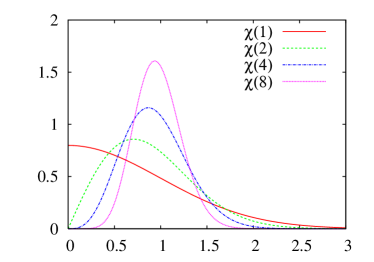
Figure 1: (Color online) Probability distributions $\chi(1),\chi(2),\chi(4),\chi(8)$ of the radius of a Gaussian vector of dimension 1, 2, 4 and 8. When the dimension goes to infinity, the distribution gets closer to a Dirac distribution.

Here we are interested in the problem of extending continuous-variable QKD over longer distances without post-selection, but with proven security. The main idea is as follows : whereas Gaussian random values are centered around $0$, this is not the case for the norm of a Gaussian random vector. Such a vector lies indeed on a shell which gets thinner as the dimension of the space increases (see Fig. 1). Thus, if one performs a clever rotation (see Fig. 2) before encoding the key in the sign of the coordinates, one automatically gets rid of the small absolute value coordinates without post-selection. Whereas this effect gets stronger and stronger for large dimensions, we will show that we are intrinsically limited to performing such rotations in $\mathbb{R}^{8}$. As we will show below, this is related to the algebraic structure of octonions. For our purpose, working in $\mathbb{R}^{8}$ is already a significant improvement since it allows to exchange secure secret keys over more than 50 km, without post-selection, and with a reasonable complexity for the reconciliation protocol.

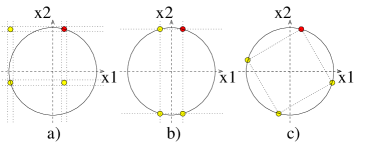
Figure 2: (Color online) Consider two successive states $X_{1},X_{2}$ sent by Alice: the states really sent correspond to $X_{1}>0,X_{2}>0$. Figures a), b) and c) show the four possible states Bob needs to discriminate after Alice has sent him some side information over the classical authenticated channel. a) corresponds to slice reconciliation Van Assche et al. (2004); Bloch et al. (2006): the four states are well separated but the Gaussian symmetry is broken, b) corresponds to the case where the information is encoded on the sign of the Gaussian value Silberhorn et al. (2002): the symmetry of the problem is preserved but some states are very close and thus difficult to discriminate, c) corresponds to the approach presented in this paper where the states are well separated and the symmetry is preserved.

The paper is organized as follows: Section II presents the link between the reconciliation and the security of the protocol, Sec. III describes the reconciliation in the case of discrete variables QKD protocols, Sec. IV shows how to generalize this approach to Gaussian variables protocols, and Sec. V presents a realistic reconciliation protocol for continuous-variable QKD, whose performance is analyzed in Sec. VI.

II Reconciliation and security

Let $x$ and $y$ be the classical random variables associated with the measured quantities of the legitimate parties Alice and Bob, and let $E$ be the quantum state in possession of the eavesdropper. It has been shown Garcia-Patron and Cerf (2006); Navascués et al. (2006) that the theoretical secret key rate $K$ obtained using one-way reconciliation is bounded from below by

$$K\geq I(x:y)-S(x:E)\equiv K_{\text{th}}.$$

Here $I(x:y)$ and $S(x:E)$ refer, respectively, to the Shannon mutual information Cover and Thomas (1991) between classical random values $x$ and $y$ and to the quantum mutual information Nielsen and Chuang (2000) between $x$ and the quantum state $E$. Recall that $S(x:E)$ can also be seen as the Holevo quantity associated to the quantum measurements performed by Eve. The above bound corresponds to the case where Alice and Bob are "classical" whereas Eve is "quantum", which means that Eve is allowed to use a quantum memory and a quantum computer to perform her attack. This secret key rate is valid for one-way reconciliation: the classical communication between Alice and Bob is therefore restricted to be unidirectional, and not interactive. For the protocol described above, the quantum mutual information between Bob and Eve is smaller than between Alice and Eve. As a consequence, one will use reverse reconciliation Grosshans et al. (2003): the final key is extracted from Bob’s data, and Bob sends extra information to Alice on the authenticated classical channel to help her correct her "errors". The secret key rate $K_{\text{th}}$ is secure against collective attacks. Note that it is conjectured that, as it is the case for discrete variables protocols Renner (2005), coherent attacks are not more powerful than collective attacks Garcia-Patron and Cerf (2006); Navascués et al. (2006); Renner (2007), which would imply that $K_{\text{th}}$ is the secure key rate against the most general attacks allowed by quantum mechanics.

An important property of the continuous-variable QKD is that for a reasonably low excess noise (which is the noise not directly caused by the losses), $K_{\text{th}}$ remains strictly positive for any value of the transmission meaning that there is not any theoretical limitation to the range of this protocol. However $K_{\text{th}}$ is relevant only in the case where one has access to a perfect reconciliation scheme, allowing Alice and Bob to extract all the information available in their correlated data. How should $K_{\text{th}}$ be modified in the case of a real-world imperfect reconciliation scheme? In order to extract a secret from their data, Alice and Bob have access to a classical authenticated channel and have agreed on a particular code $\mathcal{C}_{N}$ whose size $N$ is such that $\log_{2}(N)\leq I(x;y)$. The principle of the reconciliation protocol is the following: Alice chooses randomly an element $U\in\mathcal{C}_{N}$ and sends some information $\alpha$ to Bob who should be able to efficiently recover $U$ from the knowledge of $y$ and $\alpha$, i.e., $H(U|y,\alpha)=0$, the conditional entropy of $U$ given $y$ and $\alpha$ is null, or equivalently $I(U:y,\alpha)=H(U)$. In this case, Alice and Bob have extracted a common string $U$ from their data, which they will be able to turn into a secret key thanks to privacy amplification, but they have also given the extra information $\alpha$ to the eavesdropper. As a consequence, the effective key rate after the reconciliation becomes:

$$K\geq H(U)-S(U:E,\alpha)\equiv K_{\text{real}}.$$

Unfortunately, one always has $K_{\text{real}}<K_{\text{th}}$ and $K_{\text{real}}$ reaches $0$ for a finite channel transmission. In other words, the range of the protocol is limited because of the imperfect reconciliation. It should be noted that this is one of the main differences with discrete variables protocols which are limited by technology, and more particularly by the dark counts of the photodetectors. A real difficulty lies in the estimation of $S(U:E,\alpha)$. One specificity of QKD is that it allows Alice and Bob to estimate an upper bound of $S(x:E)$ by comparing a subset of their data. However it is generally impossible to deduce $S(U:E,\alpha)$ from it. One exception is when $U$ and $\alpha$ are independent, in which case the following lemma applies.

Lemma 1.

Let $A$ and $B$ be two classical random values, let $E$ be a random quantum state. If $A$ and $B$ are independent, then $S(A:E,B)\leq S(A,B:E)$.

Proof.

The chain rule for mutual quantum information reads:

$$S(A,B:E)=S(B:E)+S(A:E|B)\geq S(A:E|B)$$

where the inequality results from the non-negativity of mutual quantum information. Then, by definition of conditional mutual information,

$$S(A:E|B) = S(A|B)-S(A|E,B)=S(A)-S(A|E,B)$$

$$= S(A:E,B)$$

where the second equality follows from independence of $A$ and $B$. ∎

In the reconciliation protocol, $U$ is chosen randomly by Alice, independently of $x$, meaning that $S(x,U:E)=S(x:E)$. Then, since $\alpha$ is a function of $x$ and $U$, the data-processing inequality gives $S(U,\alpha:E)\leq S(x:E)$. In addition, in the case where $\alpha$ is independent of $U$, lemma (1) gives: $S(U:E,\alpha)\leq S(x:E).$

If one defines the efficiency of reconciliation $\beta=\frac{H(U)}{I(x:y)}$, one obtains finally

$$K_{\text{real}}\geq\beta I(x:y)-S(x:E),$$

which is the usual expression of the secret key rate taking into account the imperfect reconciliation protocol.

III Reconciliation of binary variables

Reconciliation is a means for Alice and Bob to extract available common information from their correlated data. In the case when the data consists of binary strings, it is very similar to the problem of channel coding where the goal is for Alice to send information to Bob through a noisy channel. Channel coding is solved by appropriately choosing subsets of binary strings: codes. When Alice restricts her messages to code words, Bob can recover them with high probability if the code size is not too large, given the channel noise. More precisely, Shannon’s theorem Shannon (1948) states that the size of the code $|\mathcal{C}|$ is bounded by the mutual information between Alice and Bob: $\log_{2}(|\mathcal{C}|)\leq I(x:y)$. The problem of channel coding has been extensively studied during the past 60 years, but only recently were discovered codes almost achieving Shannon’s limit while being efficiently decoded thanks to iterative algorithms: turbocodes Berrou et al. (1993) and Low Density Parity Check (LDPC) codes Richardson et al. (2001).

The main difference between reconciliation and channel coding is that in the case of reconciliation, Alice does not choose what she sends and thus cannot restrict her messages to code words of a given code. However, if one wants to take advantage of the code formalism, knowing what she sent, Alice can describe to Bob a code for which her word is a code word. Thus if Bob can guess what codeword Alice sent, they will effectively share a common sequence of bits. This is the method used for discrete QKD protocols. Indeed, given a linear code $\mathcal{C}$ and its parity check matrix $H$, the group $\mathbb{F}_{2}^{n}=\{0,1\}^{n}$ of possible states sent by Alice can be seen as the product of code words and syndromes: if Alice sends $x$ to Bob, she can tell him the syndrome of $x$ which is $H\cdot x$ thus defining a coset code containing $x$. This coset code is the ensemble: $\{y\in\mathbb{F}_{2}^{n}|H\cdot y=x\}$. An equivalent solution is for Alice to randomly choose a code word $U$ from a given code and to send $U\oplus x=\alpha$ to Bob where $\oplus$ represents the addition in the group $\mathbb{F}_{2}^{n}$. Bob then computes $y\oplus\alpha$ which allows him to retrieve $U$ if the code is well adapted to the channel between Alice and Bob. This coset coding scheme was initially suggested by Wyner Wyner (1975).

In a way, the side information (information sent by Alice over the classical authenticated channel) corresponds to a change of coordinates allowing one to transform the initial reconciliation problem into the well-known problem of channel coding.

Two properties are essential for this approach to work: first, the probability distribution of the states sent by Alice is uniform over $\mathbb{F}_{2}^{n}$; second, the total space is a partition of the cosets of a linear code. Thus, any word can be seen as a unique codeword for a unique coset code and telling which coset code contains the word gives zero information about the codeword. The question is then whether or not it is possible to generalize this approach to continuous variables.

IV Reconciliation of Gaussian variables

IV.1 Gaussian modulation

One of the main differences between discrete and continuous QKD protocols is the probability distribution of Alice’s variables: the uniform distribution on $\mathbb{F}_{2}^{n}$ is changed into a nonuniform Gaussian distribution on $\mathbb{R}^{n}$. This is rather unfortunate since the uniformity of the distribution on $\mathbb{F}_{2}^{n}$ is an essential assumption in order to prove that the side information (e.g., the syndrome) Alice sends to Bob on the public channel does not give any relevant information to Eve about the code word chosen by Alice. An interesting property of the Gaussian distribution $\mathcal{N}(0,\mathbbm{1}_{n})$ on $\mathbb{R}^{n}$ whose covariance matrix is the identity is that it has a spherical symmetry in $\mathbb{R}^{n}$. In other words, if the vector $x$ follows such a distribution, then the normalized random vector $\frac{x}{|x|}$ has a uniform distribution on the unit sphere $\mathcal{S}^{n-1}$ of $\mathbb{R}^{n}$. Thus, spherical codes, codes for which all codewords lie on a sphere centered on $0$, can play the same role for continuous-variable protocols as binary codes for discrete protocols. Some very good codes are known for binary channels: LDPC codes and turbocodes both almost achieve the Shannon limit and can be efficiently decoded thanks to iterative decoding algorithms. Are there codes with similar qualities among the spherical codes? The answer is almost. There is indeed a canonical way to convert binary codes into binary spherical codes and this can be achieved thanks to the following mapping of $\mathbb{F}_{2}^{n}$ onto an isomorphic image in the $n$-dimensional sphere:

$$\mathbb{F}_{2}^{n}\rightarrow\mathcal{S}^{n-1}\subset\mathbb{R}^{n},(b_{1},\dots,b_{n})\mapsto\left(\frac{(-1)^{b_{1}}}{\sqrt{n}},\dots,\frac{(-1)^{b_{n}}}{\sqrt{n}}\right).$$

Then, as LDPC codes and turbocodes can both be optimized for binary symmetric channels, they can also be optimized for a binary phase shift keying (BPSK) modulation, where the bit $0$ $(1)$ is encoded into the amplitude $+A$ $(-A)$, and where the channel noise is considered to be additive white Gaussian noise (AWGN). Thus, one has access to a family of very good codes (in the sense that they are very close to the Shannon limit) for which very efficient iterative decoding algorithms are available. It is important to note that there are actually two different Shannon limits considered here depending on the modulation, BPSK or Gaussian modulation, but these limits become asymptotically close when the signal-to-noise ratio (SNR) is small. Thus, at low SNR, a binary code optimized for a BPSK modulation can almost achieve the Shannon limit for a Gaussian modulation.

A remark is in order : the use of binary codes as described above limits the rate of the code to less than $1$ bit per channel use, whereas one of the interests of a Gaussian modulation is precisely to get rid of this limit. Actually, one could use nonbinary spherical codes, but their decoding is more complicated and thus slows down the reconciliation protocol. In addition, this is not really needed, since in the high loss scenario which interests us most here, the secret key rate is always much less than 1 bit per channel use. Consequently the use of binary codes turns into an advantage, since they can be decoded very efficiently. In the low-loss case however, that is for short distances, one can hope to distill more than $1$ bit per channel use, and the "usual" approach Lodewyck et al. (2007) will be more suitable than the one described in the present article (see also discussion in Sec. VI).

Now that we have a probabilistic space with a uniform probability distribution and a family of codes for this space, we need to see if the total space is a partition of a code and of its "generalized coset codes". First, the canonical hypercube of $\mathbb{R}^{n}$ (which is the image of $\mathbb{F}_{2}^{n}$ by the isomorphism defined above) is described as a partition of a linear code and its cosets. The question that remains to be solved is whether or not the unit sphere is a partition of such hypercubes. Another way to see this problem is the following: given a random point in $\mathcal{S}^{n-1}$, is there a hypercube inscribed in the sphere for which this point is a vertex. Surely there are such hypercubes, many in fact. Actually, the manifold of these hypercubes is a $[(n-1)(n-2)/2]$-dimensional manifold (this is the dimension of the subgroup of orthogonal group $O_{n}$ that transports the canonical hypercube onto the ensemble of hypercubes containing the point in question).

Yet another way to express the problem is the following: given two points $x,y\in\mathcal{S}^{n-1}$, is it possible to find an orthogonal transformation mapping $x$ to $y$? One can immediately think of transformations such as the reflection across the mediator hyperplane of $x$ and $y$. Unfortunately, such an orthogonal transformation gives some information about $x$ and $y$ as soon as $n>2$ (this is linked to the phenomenon of concentration of measure for spheres in dimensions $n>2$), and therefore cannot be used by Alice as legitimate side information, which should be independent from the key in order to fulfill the hypothesis of Lemma 1.

A correct solution would then be to randomly choose an orthogonal transformation with uniform probability in the ensemble of orthogonal transformations mapping $x$ to $y$. This can be done in the following way: one first draws a random orthogonal transformation mapping $x$ to some random $x^{\prime}$. Then one composes this transformation with the reflection across the mediator hyperplane of $x^{\prime}$ and $y$. Although theoretically correct, this procedure is not doable in practice for $n\gg 1$ since generating a random orthogonal transformation on $\mathbb{R}^{n}$ is a computational demanding task requiring to draw an $n\times n$ Gaussian random matrix and to calculate its QR decomposition (i.e., its decomposition into an orthogonal and a triangular matrix) which is an operation of complexity $O(n^{3})$.

A practical solution involves the following: for each word $x\in\mathcal{S}^{n-1}$ sent by Alice, for each code word $U\in\mathcal{S}^{n-1}$ chosen by Alice (not necessarily a binary codeword), there should exist an continuous application $M$ of the variables $x$ and $U$ such that $M(x,U)\in O_{n}$ and $M(x,U)\cdot x=U$. Then if Alice gives $M(x,U)$ to Bob, one has the continuous equivalent of $U\oplus x$ in the discrete protocol. The following theorem shows that the existence of such an application $M$ restricts the possible values of $n$ to be $1$, $2$, $4$ or $8$.

Theorem 2.

If there exists a continuous application

$$M:\mathcal{S}^{n-1}\times\mathcal{S}^{n-1}\rightarrow O_{n},(x,y)\mapsto M(x,y)$$

such that $M(x,y)\cdot x=y$ for all $x,y\in\mathcal{S}^{n-1}$, then $n=$ $1$, $2$, $4$ or $8$.

The proof of this theorem uses a result from Adams Adams (1962), which quantifies the number of independent vector fields on the unit sphere of $\mathbb{R}^{n}$:

Theorem 3.

Independent vector fields on $\mathcal{S}^{n-1}$ (J.F. Adams, 1962). For $n=a\cdot 2^{b}$ with $a$ odd and $b=c+4d$, one defines $\rho_{n}=2^{c}+8d$. Then the maximal number of linearly independent vector fields on $\mathcal{S}^{n-1}$ is $\rho_{n}-1$.

In particular, the only spheres for which there exist $(n-1)$ independent vector fields are the unit sphere of $\mathbb{R}$, $\mathbb{R}^{2}$, $\mathbb{R}^{4}$ and $\mathbb{R}^{8}$, which can respectively be seen as the units of the real numbers, the complex numbers, the quaternions and the octonions.

Proof of Theorem 2..

The idea of the proof is to use the existence of such a continuous function $M$ to exhibit a family of $(n-1)$ independent vector fields on $S^{n-1}$.

Let $(e_{1},e_{2},\dots,e_{n})$ be the canonical orthonormal basis of $\mathbb{R}^{n}$. For $1\leq i\leq n$, let $u_{i}(x)=M(e_{n},x)\cdot e_{i}$. One has: $u_{n}(x)=x$ and

$$(u_{i}(x)|u_{j}(x)) = e_{i}^{T}M(e_{n},x)^{T}M(e_{n},x)e_{j}$$

$$= \delta_{i,j}\hskip 28.45274pt\text{since $M(e_{n},x)\in O_{n}$}$$

Then, for $x\in\mathcal{S}^{n-1}$, $u_{1}(x),u_{2}(x),\dots,u_{n-1}(x)$ are $(n-1)$ independent vector fields on $\mathcal{S}^{n-1}$ and finally $n=1,2,4$ or $8$. ∎

V Rotations on $\mathcal{S}^{1}$, $\mathcal{S}^{3}$ and $\mathcal{S}^{7}$

Now that we have proved that such an application $M$ can only exist in $\mathbb{R}$, $\mathbb{R}^{2}$, $\mathbb{R}^{4}$ and $\mathbb{R}^{8}$, we need to answer three more questions: does it exist? Can Alice compute it efficiently? Does it leak any information about the codeword to Eve? Note that the trivial case of $\mathbb{R}$ for which the unit sphere is $\{-1,1\}$ corresponds to the method where one encodes a bit in the sign of the Gaussian variable Silberhorn et al. (2002).

V.1 Existence

Let us start with the easiest case: $\mathbb{R}^{2}$. The existence of such an application $M$ verifying $M(x,y)\cdot x=y$ for the unit circle is obvious: it is simply the rotation centered in $O$ of angle $\text{Arg}(y)-\text{Arg}(x)$ where Arg$(x)$ denotes the angle between $x$ and the x-axis. An alternative way to see $M$ is $M(x,y)=yx^{-1}$ where $x$ and $y$ are identified with complex numbers of modulus $1$. The same is true for dimensions $4$ and $8$ where $\mathcal{S}^{3}$ and $\mathcal{S}^{7}$ can respectively be identified with the quaternion units and the octonion units, and for which a valid division exists.

V.2 Computation of $M(x,y)$

For $n=2,4$ and $8$, there exists a (nonunique) family of $n$ orthogonal matrices $\mathcal{A}_{n}=(A_{1},\dots,A_{n})$ of $\mathbb{R}^{n\times n}$ such that $A_{1}=\mathbbm{1}_{n}$, and for $i,j>1$, $\{A_{i},A_{j}\}=-2\delta_{i,j}\mathbbm{1}_{n}$ where $\{A,B\}$ is the anticommutator of $A$ and $B$. An example of these families is explicitly given in the Appendix. The following lemma shows how to use such a family to construct a continuous function $M$ with the properties described above.

Lemma 4.

$\displaystyle{M(x,y)=\sum_{i=1\dots n}\alpha_{i}(x,y)A_{i}}$ with $\alpha_{i}(x,y)=(A_{i}x|y)$ is a continuous map from $\mathcal{S}^{n-1}\times\mathcal{S}^{n-1}$ to $O(n)$ such that $M(x,y)x=y$.

Proof.

First, because of the anticommutation property, one can easily check that the family $(A_{1}x,A_{2}x,\dots,A_{n}x)$ is an orthonormal basis of $\mathbb{R}^{n}$ for any $x\in\mathcal{S}^{n-1}$. Then, for any $x,y\in\mathcal{S}^{n-1}$, $(\alpha_{1}(x,y),\dots,\alpha_{n}(x,y))$ are the coordinates of $y$ in the basis $(A_{1}x,A_{2}x,\dots,A_{n}x)$. This proves that $M(x,y)x=y$. Finally, the orthogonality of $M(x,y)$ follows from some simple linear algebra. ∎

Then $\alpha=(\alpha_{1},\dots,\alpha_{n})$ is sufficient to describe $M(x,y)$ and the computation of $\alpha_{i}$ can be done efficiently since the matrices $A_{i}$ are just permutation matrices with a change of sign for some coordinates. In the QKD protocol, Alice chooses randomly $u$ in a finite code and gives the value of $\alpha(x,u)$ to Bob, who is then able to compute $M(x,u)y$ which is a noisy version of $u$. One should note that the final noise is just a "rotated" version of the noise Bob has on $x$: in particular, both noises are Gaussian with the same variance.

V.3 No leakage of information

In order to prove that $\alpha=M(x,u)$ does not give any information about $u$, one needs to show that $u$ and $\alpha$ are independent, in other words that: $Pr(u=u_{i}|M(x,u)=\alpha)=Pr(u=u_{i})=\frac{1}{N}$ if one considers the spherical code $\mathcal{C}_{N}=\{u_{1},\dots,u_{N}\}$. This is true because $x$ and $u$ have uniform distributions (on $\mathcal{S}^{n-1}$ and $\mathcal{C}_{N}$ respectively) and because the function:

$$f_{u}:\mathbb{R}^{n}\rightarrow\mathbb{R}^{n},x\mapsto f_{u}(x)=\alpha,\text{ with }\alpha_{i}=(u|A_{i}x)$$

has a constant Jacobian equal to $1$ for each $u\in\mathcal{C}_{N}$. To see this, one should note that the lines of the Jacobian matrix of $f_{u}$ are the $A_{i}^{T}u$ which form an orthonormal basis of $\mathbb{R}^{n}$.

VI Application to the continuous-variable QKD

Now that we have explained how efficient reconciliation of correlated Gaussian variables can be achieved with rotations in $\mathbb{R}^{8}$, let us look at the implications for the continuous-variable QKD.

At the end of the quantum part of the continuous-variable QKD protocol, Alice and Bob share correlated random values and their correlation depends on the variance of the modulation of the coherent states and on the properties of the quantum channel. The channel can safely be assumed to be Gaussian since it corresponds to the case of the optimal attack for Eve. This means that it can be entirely characterized by its transmission and excess noise. Both these parameters are accessible to Alice and Bob through an estimation step prior to the reconciliation Renner (2005). Once these parameters are known, one can calculate the signal-to-noise ratio (SNR) of the transmission, which is the ratio between the variance of the signal (the variance of the Gaussian modulation of coherent states in our case) and the variance of the noise (noise induced by losses as well as excess noise). The SNR quantifies the mutual information between Alice and Bob when a Gaussian modulation is sent over a Gaussian channel:

$$I(A:B)=\frac{1}{2}\log_{2}(1+\text{SNR}).$$

Note also that the efficiency of the reconciliation only depends on the correlation between Alice’s and Bob’s data, that is, on the SNR. Thus, for a given transmission and excess noise, the secret key rate is a function of the SNR, which can be optimized by changing the variance of the modulation of the coherent states.

It is not easy to know exactly how the efficiency of reconciliation depends on the SNR. However, each reconciliation technique performs better for a certain range of SNR: slice reconciliation is usually used for a SNR around $3$ Lodewyck et al. (2007) while rotations in $\mathbb{R}^{8}$ are optimal for a low SNR, typically around $0.5$.

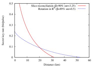
Figure 3: (Color online) Performance of slice reconciliation vs rotation in $\mathbb{R}^{8}$. Experimental parameters: excess noise referred to the channel input $\xi=0.005$, efficiency of Bob’s detector $\eta=0.606$ and electronic noise at Bob’s side $V_{elec}=0.041$ Lodewyck et al. (2007). The reconciliation based on rotations in $\mathbb{R}^{8}$ uses a LDPC code of rate 0.26 http://ltchwww.epfl.ch/research/ldpcopt

Figure 3 shows the performance of rotations in $\mathbb{R}^{8}$ compared to slice reconciliation for the experimental parameters of the QKD system developed at Institut d’Optique. Both approaches achieve comparable reconciliation efficiencies (around $90\%$) but for different SNR. One can observe two distinct regimes: for low loss, i.e., short distance, slice reconciliation is better but only rotations in $\mathbb{R}^{8}$ allow QKD over longer distances (over 50 km with the current experimental parameters).

Concerning the complexity of the reconciliation, one should be aware that almost all the computing time is devoted to decoding the efficient binary codes, either LDPC codes or turbocodes. Compared to this decoding, the rotation in $\mathbb{R}^{8}$ takes a negligible amount of time. Thus, the complexity of the reconciliation presented here is smaller than the one of slice reconciliation since the latter uses several codes (one code per slice).

VII Conclusion

We presented a protocol for the reconciliation of correlated Gaussian variables. Currently, the main bottleneck of continuous-variable QKD lies in the impossibility for Alice and Bob to extract efficiently all the information available, this difficulty resulting in both a limited range and a limited rate for the key distribution. The method described in this article is particularly well adapted for low signal-to-noise ratios, which is the situation encountered when one wants to perform QKD over long distances. By taking into account the current experimental parameters of the QKD link developed at the Institut d’Optique Lodewyck et al. (2007), one shows that this new reconciliation allows QKD over more than 50 km. Moreover, contrary to other protocols that have been proposed to increase the range of continuous-variable QKD, this protocol does not require any post-selection. Hence, the security proofs based on the optimality of Gaussian attacks Garcia-Patron and Cerf (2006); Navascués et al. (2006) remain valid, meaning that the protocol is secure against general collective attacks.

*

Appendix A Examples of families $\mathcal{A}_{2}$, $\mathcal{A}_{4}$ and $\mathcal{A}_{8}$

A.1 Notations

Let us introduce the following 4 $2\times 2$ matrices:
$K_{0}=\begin{pmatrix}1&0\\ 0&1\end{pmatrix},K_{1}=\begin{pmatrix}0&1\\ 1&0\end{pmatrix},K_{2}=\begin{pmatrix}0&-1\\ 1&0\end{pmatrix}$ and $K_{3}=\begin{pmatrix}1&0\\ 0&-1\end{pmatrix}$ and the tensor product $K_{i_{1},..,i_{l}}=K_{i_{1}}\otimes..\otimes K_{i_{l}}$.

A.2 Examples

Family $\mathcal{A}_{2}$: $\{K_{0},K_{2}\}$

$A_{1}=\begin{pmatrix}1&0\\ 0&1\end{pmatrix},A_{2}=\begin{pmatrix}0&-1\\ 1&0\end{pmatrix}$

Family $\mathcal{A}_{4}$: $\{K_{00},K_{32},K_{20},K_{12}\}$

$A_{1}=\begin{pmatrix}1&0&0&0\\ 0&1&0&0\\ 0&0&1&0\\ 0&0&0&1\\ \end{pmatrix},A_{2}=\begin{pmatrix}0&-1&0&0\\ 1&0&0&0\\ 0&0&0&1\\ 0&0&-1&0\\ \end{pmatrix},$

$A_{3}=\begin{pmatrix}0&0&-1&0\\ 0&0&0&-1\\ 1&0&0&0\\ 0&1&0&0\\ \end{pmatrix},A_{4}=\begin{pmatrix}0&0&0&-1\\ 0&0&1&0\\ 0&-1&0&0\\ 1&0&0&0\\ \end{pmatrix}$

Family $\mathcal{A}_{8}$: $\{K_{000},K_{332},K_{320},K_{312},K_{200},K_{102},K_{123},K_{121}\}$

$A_{1}=\begin{pmatrix}1&0&0&0&0&0&0&0\\ 0&1&0&0&0&0&0&0\\ 0&0&1&0&0&0&0&0\\ 0&0&0&1&0&0&0&0\\ 0&0&0&0&1&0&0&0\\ 0&0&0&0&0&1&0&0\\ 0&0&0&0&0&0&1&0\\ 0&0&0&0&0&0&0&1\\ \end{pmatrix},$

$A_{2}=\begin{pmatrix}0&-1&0&0&0&0&0&0\\ 1&0&0&0&0&0&0&0\\ 0&0&0&1&0&0&0&0\\ 0&0&-1&0&0&0&0&0\\ 0&0&0&0&0&1&0&0\\ 0&0&0&0&-1&0&0&0\\ 0&0&0&0&0&0&0&-1\\ 0&0&0&0&0&0&1&0\\ \end{pmatrix},$

$A_{3}=\begin{pmatrix}0&0&-1&0&0&0&0&0\\ 0&0&0&-1&0&0&0&0\\ 1&0&0&0&0&0&0&0\\ 0&1&0&0&0&0&0&0\\ 0&0&0&0&0&0&1&0\\ 0&0&0&0&0&0&0&1\\ 0&0&0&0&-1&0&0&0\\ 0&0&0&0&0&-1&0&0\\ \end{pmatrix},$

$A_{4}=\begin{pmatrix}0&0&0&-1&0&0&0&0\\ 0&0&1&0&0&0&0&0\\ 0&-1&0&0&0&0&0&0\\ 1&0&0&0&0&0&0&0\\ 0&0&0&0&0&0&0&1\\ 0&0&0&0&0&0&-1&0\\ 0&0&0&0&0&1&0&0\\ 0&0&0&0&-1&0&0&0\\ \end{pmatrix},$

$A_{5}=\begin{pmatrix}0&0&0&0&-1&0&0&0\\ 0&0&0&0&0&-1&0&0\\ 0&0&0&0&0&0&-1&0\\ 0&0&0&0&0&0&0&-1\\ 1&0&0&0&0&0&0&0\\ 0&1&0&0&0&0&0&0\\ 0&0&1&0&0&0&0&0\\ 0&0&0&1&0&0&0&0\\ \end{pmatrix},$

$A_{6}=\begin{pmatrix}0&0&0&0&0&-1&0&0\\ 0&0&0&0&1&0&0&0\\ 0&0&0&0&0&0&0&-1\\ 0&0&0&0&0&0&1&0\\ 0&-1&0&0&0&0&0&0\\ 1&0&0&0&0&0&0&0\\ 0&0&0&-1&0&0&0&0\\ 0&0&1&0&0&0&0&0\\ \end{pmatrix},$

$A_{7}=\begin{pmatrix}0&0&0&0&0&0&-1&0\\ 0&0&0&0&0&0&0&1\\ 0&0&0&0&1&0&0&0\\ 0&0&0&0&0&-1&0&0\\ 0&0&-1&0&0&0&0&0\\ 0&0&0&1&0&0&0&0\\ 1&0&0&0&0&0&0&0\\ 0&-1&0&0&0&0&0&0\\ \end{pmatrix},$

$A_{8}=\begin{pmatrix}0&0&0&0&0&0&0&-1\\ 0&0&0&0&0&0&-1&0\\ 0&0&0&0&0&1&0&0\\ 0&0&0&0&1&0&0&0\\ 0&0&0&-1&0&0&0&0\\ 0&0&-1&0&0&0&0&0\\ 0&1&0&0&0&0&0&0\\ 1&0&0&0&0&0&0&0\\ \end{pmatrix}.\\$

References

- Gisin et al. (2002) N. Gisin, G. Ribordy, W. Tittel, and H. Zbinden, Rev. Mod. Phys. 74, 145 (2002).
- Grosshans et al. (2003) F. Grosshans, G. V. Assche, J. Wenger, R. Brouri, N. J. Cerf, and P. Grangier, Nature 421, 238 (2003).
- Bennett et al. (1984) C. Bennett, G. Brassard, et al., Proceedings of IEEE International Conference on Computers, Systems, and Signal Processing 175 (1984).
- Van Assche et al. (2004) G. Van Assche, J. Cardinal, and N. J. Cerf, IEEE Transactions on Information Theory 50, 394 (2004).
- Bloch et al. (2006) M. Bloch, A. Thangaraj, S. W. McLaughlin, and J.-M. Merolla, in Proc. IEEE Information Theory Workshop (Punta del Este, Uruguay, 2006), arXiv:cs.IT/0509041.
- Ralph (2000) T. C. Ralph, Phys. Rev. A 61, 010303(R) (2000).
- Silberhorn et al. (2002) C. Silberhorn, T. Ralph, N. Lütkenhaus, and G. Leuchs, Phys. Rev. Lett. 89, 167901 (2002).
- Weedbrook et al. (2004) C. Weedbrook, A. Lance, W. Bowen, T. Symul, T. Ralph, and P. Lam, Phys. Rev. Lett. 93, 170504 (2004).
- Namiki and Hirano (2004) R. Namiki and T. Hirano, Phys. Rev. Lett. 92, 117901 (2004).
- Weedbrook et al. (2005) C. Weedbrook, A. Lance, W. Bowen, T. Symul, T. Ralph, and P. Lam, Phys. Rev. Lett. 95, 180503 (2005).
- Heid and Lütkenhaus (2007) M. Heid and N. Lütkenhaus, Phys. Rev. A 76, 022313 (2007), eprint arXiv:quant-ph/0608015.
- Garcia-Patron and Cerf (2006) R. Garcia-Patron and N. J. Cerf, Phys. Rev. Lett. 97, 190503 (2006).
- Navascués et al. (2006) M. Navascués, F. Grosshans, and A. Acín, Phys. Rev. Lett. 97, 190502 (2006).
- Cover and Thomas (1991) T. M. Cover and J. A. Thomas, Elements of Information Theory (Wiley-Interscience, 1991).
- Nielsen and Chuang (2000) M. A. Nielsen and I. L. Chuang, Quantum Information and Quantum Computation (Cambridge University Press, 2000).
- Renner (2005) R. Renner, Ph.D. thesis, ETH Zurich (2005).
- Renner (2007) R. Renner, Nature Physics 3, 645 (2007).
- Shannon (1948) C. Shannon, Bell System Technical Journal 27, 379 (1948).
- Berrou et al. (1993) C. Berrou, A. Glavieux, and P. Thitimajshima, Communications, 1993. ICC 93. Geneva. Technical Program, Conference Record, IEEE International Conference on 2 (1993).
- Richardson et al. (2001) T. J. Richardson, M. A. Shokrollahi, and R. L. Urbanke, IEEE Transactions on Information Theory 47, 619 (2001).
- Wyner (1975) A. D. Wyner, Bell System Technical Journal 54, 1355 (1975).
- Lodewyck et al. (2007) J. Lodewyck, M. Bloch, R. García-Patrón, S. Fossier, E. Karpov, E. Diamanti, T. Debuisschert, N. J. Cerf, R. Tualle-Brouri, S. W. McLaughlin, et al., Phys. Rev. A 76, 042305 (2007).
- Adams (1962) J. Adams, Annals of Math. 75, 603 (1962).
- (24) http://ltchwww.epfl.ch/research/ldpcopt.