CoRoT/ESTA–TASK 1 and TASK 3 comparison of the internal structure and seismic properties of representative stellar models

Abstract

We compare stellar models produced by different stellar evolution codes for the CoRoT/ESTA project, comparing their global quantities, their physical structure, and their oscillation properties. We discuss the differences between models and identify the underlying reasons for these differences. The stellar models are representative of potential CoRoT targets. Overall we find very good agreement between the five different codes, but with some significant deviations. We find noticeable discrepancies (though still at the per cent level) that result from the handling of the equation of state, of the opacities and of the convective boundaries. The results of our work will be helpful in interpreting future asteroseismology results from CoRoT.

1 Introduction

The goals of ESTA-TASKs 1 and 3 are to test the numerical tools used in stellar modelling, with the objective to be ready to interpret safely the asteroseismic data that will come from the CoRoT mission. This consists in quantifying the effects of different numerical implementations of the stellar evolution equations and related input physics on the internal structure, evolution and seismic properties of stellar models. As a result, we aim at improving the stellar evolution codes to get a good agreement between models built with different codes and same input physics. For that purpose, several study cases have been defined that cover a large range of stellar masses and evolutionary stages and stellar models have been calculated without (in TASK 1) or with (in TASK 3) microscopic diffusion (see Monteiro et al., 2006; Lebreton et al., 2007a).

In this paper, we present the results of the detailed comparisons of the internal structures and seismic properties of TASKs 1 and 3 target models. The comparisons of the global parameters and evolutionary tracks are discussed in Monteiro et al. (2007). In order to ensure that the differences found are mainly determined by the way each code calculates the evolution and the structure of the model and not by significant differences in the input physics, we decided to use and compare models whose global parameters (age, luminosity, and radius) are very similar. Therefore, we selected models computed by five codes among the ten participating in ESTA: ASTEC (Christensen-Dalsgaard, 2007a), CESAM (Morel and Lebreton, 2007), CLÉS (Scuflaire et al., 2007a), GARSTEC (Weiss and Schlattl, 2007), and STAROX (Roxburgh, 2007).

In Section 2 we recall the specifications of TASKs 1 and 3 and present the five codes used in the present paper. We then present the comparisons for TASK 1 in Sect. 3 and for TASK 3 in Sect. 4. For each case in each task, we have computed the relative differences of the physical quantities between pairs of models. We display the variation of the differences between the more relevant quantities inside the star and we provide the average and extreme values of the variations. We then compare the location of the boundaries of the convective regions as well as their evolution with time. For models including microscopic diffusion we examine how helium is depleted at the surface as a function of time. Finally, we analyse the effect of internal structure differences on seismic properties of the model.

2 Presentation of the ESTA-TASKs and tools

In the following we briefly recall the specifications and tools of TASK 1 and TASK 3 that have been presented in detail by Lebreton et al. (2007a).

2.1 TASK 1: basic stellar models

The specifications for the seven cases that have been considered in TASK 1 are recalled in Table 2.1. For each case, evolutionary sequences have been calculated for the specified values of the stellar mass and initial chemical composition ($X,Y,Z$ where $X$, $Y$ and $Z$ are respectively the initial hydrogen, helium and metallicity in mass fraction) up to the evolutionary stage specified. The masses are in the range $0.9-5.0$ $\,{M}_{\odot}$. For the initial chemical composition, different $(Y,Z)$ couples have been considered by combining two different values of $Z$ ($0.01$ and $0.02$) and two values of $Y$ ($0.26$ and $0.28$). The evolutionary stages considered are either on the pre main sequence (PMS), the main sequence (MS) or the subgiant branch (SGB). On the PMS the central temperature of the model ($T_{\mathrm{c}}=1.9\times 10^{7}\ {\mathrm{K}}$) has been specified. On the MS, the value of the central hydrogen content has been fixed: $X_{\mathrm{c}}=0.69$ for a model close to the zero age main sequence (ZAMS), $X_{\mathrm{c}}=0.35$ for a model in the middle of the MS and $X_{\mathrm{c}}=0.01$ for a model close to the terminal age main sequence (TAMS). On the SGB, a model is chosen by specifying the value of the mass $M_{\mathrm{c}}^{\mathrm{He}}$ of the central region of the star where the hydrogen abundance is such that $X\leq 0.01$. We chose $M_{\mathrm{c}}^{\mathrm{He}}=0.10$ $\,{M}_{\odot}$.

All models calculated for TASK 1 are based on rather simple input physics, currently implemented in stellar evolution codes and one model has been calculated with overshooting. Also, reference values of some astronomical and physical constants have been fixed as well as the mixture of heavy elements to be used. These specifications are described in Lebreton et al. (2007a).

Table 1: Target models for TASK 1. We have considered 7 cases corresponding to different initial masses, chemical compositions and evolutionary stages. One evolutionary sequence (denoted by “OV” in the $\rm{5^{th}}$ column has been calculated with core overshooting (see text).

Case	$M/M_{\odot}$	$Y_{0}$	$Z_{0}$	Specification	Type
1.1	0.9	0.28	0.02	$X_{\mbox{\scriptsize c}}{=}0.35$	MS
1.2	1.2	0.28	0.02	$X_{\mbox{\scriptsize c}}{=}0.69$	ZAMS
1.3	1.2	0.26	0.01	$M^{\mbox{\scriptsize He}}_{\mbox{\scriptsize c}}{=}0.10$ $\,{M}_{\odot}$	SGB
1.4	2.0	0.28	0.02	$T_{\mbox{\scriptsize c}}{=}1.9{\times}10^{7}$ K	PMS
1.5	2.0	0.26	0.02	$X_{\mbox{\scriptsize c}}{=}0.01,{\mbox{OV}}$	TAMS
1.6	3.0	0.28	0.01	$X_{\mbox{\scriptsize c}}{=}0.69$	ZAMS
1.7	5.0	0.28	0.02	$X_{\mbox{\scriptsize c}}{=}0.35$	MS

2.2 TASK 3: stellar models including microscopic diffusion

TASK 3 is dedicated to the comparisons of stellar models including microscopic diffusion of chemical elements resulting from pressure, temperature and concentration gradients (see Thoul and Montalbán, 2007). The other physical assumptions proposed as the reference for the comparisons of TASK 3 are the same as used for TASK 1, and no overshooting.

Three study cases have been considered for the models to be compared. Each case corresponds to a given value of the stellar mass (see Table 2.2) and to a chemical composition close to the standard solar one ($Z/X=0.0243$). For each case, models at different evolutionary stages have been considered. We focused on three particular evolution stages : middle of the MS, TAMS and SGB (respectively stage A, B and C).

Table 2: Target models for TASK 3. Left: The 3 cases with corresponding masses and initial chemical composition. Right: The 3 evolutionary stages examined for each case. Stages A and B are respectively in the middle and end of the MS stage. Stage C is on the SGB.

Case	${\frac{M}{M_{\odot}}}$	$Y_{0}$	$Z_{0}$
3.1	$1.0$	$0.27$	$0.017$
3.2	$1.2$	$0.27$	$0.017$
3.3	$1.3$	$0.27$	$0.017$

Stage	$X_{\rm c}$	$M^{\mbox{\scriptsize He}}_{\mbox{\scriptsize c}}$
A	$0.35$	-
B	$0.01$	-
C	$0.00$	$0.05\ M_{\mathrm{star}}$

2.3 Numerical tools

Among the stellar evolution codes considered in the comparisons presented by Monteiro et al. (2007), we have considered 5 codes – listed below – for further more detailed comparisons. These codes have shown a very good agreement in the comparison of the global parameters which ensures that they closely follow the specifications of the tasks in terms of input physics and physical and astronomical constants.

• ASTEC – Aarhus STellar Evolution Code, described in Christensen-Dalsgaard (2007a).

• CESAM – Code d’Évolution Stellaire Adaptatif et Modulaire, see Morel and Lebreton (2007).

• CLÉS – Code Liégeois d’Évolution Stellaire, see Scuflaire et al. (2007a).

• GARSTEC – Garching Evolution Code, presented in Weiss and Schlattl (2007).

• STAROX – Roxburgh’s Evolution Code, see Roxburgh (2007).

The oscillation frequencies presented in this paper have been calculated with the LOSC adiabatic oscillation code (Liège Oscillations Code, see Scuflaire et al., 2007b). Part of the comparisons between the models has been performed with programs included in the Aarhus Adiabatic Pulsation Package ADIPLS (see Christensen-Dalsgaard, 2007b).

3 Comparisons for TASK 1

3.1 Presentation of the comparisons and general results

The TASK 1 models span different masses and evolutionary phases. Cases 1.1, 1.2 and 1.3 illustrate the internal structure of solar-like, low-mass $0.9$$\,{M}_{\odot}$ and $1.2$$\,{M}_{\odot}$ stars, at the beginning of the main sequence of hydrogen burning (Case 1.2), in the middle of the MS when the hydrogen mass fraction in the centre has been reduced to the half of the initial one (Case 1.1) and in the post-main sequence when the star has already built a He core of $0.1$$\,{M}_{\odot}$ (Case 1.3). Cases 1.4 and 1.5 correspond to intermediate-mass models ($2.0$$\,{M}_{\odot}$), the first one, in a phase prior to the MS when the nuclear reactions have not yet begun to play a relevant role, and the second one, at the end of the MS, when the matter in the centre contains only $1$% of hydrogen. Finally, Cases 1.6 ($3.0$$\,{M}_{\odot}$) and 1.7 ($5.0$$\,{M}_{\odot}$) sample the internal structure of models corresponding to middle and late B-type stars. For these more massive models, the beginning and the middle of their MS are examined.

The models provided correspond to a different number of mesh points: the number of mesh points is $1202$ in the ASTEC models; it is in the range $2300-3700$ in CESAM models, $2200-2400$ in CLÉS models, $1500-2100$ in models by GARSTEC and $1900-2000$ in STAROX models. As explained in the papers devoted to the description of the participating codes (Christensen-Dalsgaard, 2007a; Morel and Lebreton, 2007; Roxburgh, 2007; Scuflaire et al., 2007a; Weiss and Schlattl, 2007), the numerical methods used to solve the equations and to interpolate in the tables containing physical inputs are specific to each code and so are the possibilites to choose the number and repartition of the mesh points in a model or the time step of the evolution calculation and, more generally, the different levels of precision of the computation. The specifications for the tasks have concerned mainly the physical inputs and the constants to be used (Lebreton et al., 2007a) and have let the modelers free to tune up the numerous numerical parameters involved in their calculation which explains why each code deals with different numbers (and repartition) of mesh points.

Table 3: TASK 1 models: Global parameter differences given in per cent, between each code and CESAM. For each parameter we give the mean and maximum difference of the complete series of TASK 1 models

Code	$\delta R/R$		$\delta L/L$		$\delta T_{\rm eff}/T_{\rm eff}$
	mean	max	mean	max	mean	max
ASTEC	0.27	0.83	0.49	1.57	0.02	0.03
CLÉS	0.20	0.43	0.16	0.52	0.01	0.01
GARSTEC	0.37	0.59	0.23	0.46	0.03	0.06
STAROX	0.75	3.29	0.31	0.89	0.03	0.13

Table 4: TASK 1 models: Mean quadratic difference in the physical variables between each code and CESAM calculated according to Eq. 1. The differences are given in per cent (except for $\delta X$) and represent an average over the whole star from centre to photospheric radius. The local differences were computed at fixed relative mass.

Case 1.1
Code	$\delta\ln c$	$\delta\ln P$	$\delta\ln\rho$	$\delta\ln T$	$\delta\ln r$	$\delta\ln\Gamma_{1}$	$\delta\ln\nabla_{\rm ad}$	$\delta\ln C_{p}$	$\delta\ln\kappa$	$\delta X$	$\delta\ln L_{r}$
ASTEC	0.02	0.15	0.16	0.04	0.05	2.69$\times 10^{-4}$	5.84$\times 10^{-4}$	7.36$\times 10^{-3}$	0.44	1.2$\times 10^{-4}$	0.17
CLÉS	0.04	0.25	0.22	0.07	0.06	3.14$\times 10^{-4}$	4.06$\times 10^{-3}$	2.64$\times 10^{-2}$	0.20	3.4$\times 10^{-4}$	0.03
GARSTEC	0.06	0.40	0.44	0.07	0.09	1.46$\times 10^{-1}$	1.13$\times 10^{-1}$	1.11$\times 10^{-1}$	0.45	4.7$\times 10^{-4}$	0.33
STAROX	0.04	0.28	0.25	0.08	0.09	6.47$\times 10^{-4}$	—	—	—	3.1$\times 10^{-4}$	0.08
Case 1.2
Code	$\delta\ln c$	$\delta\ln P$	$\delta\ln\rho$	$\delta\ln T$	$\delta\ln r$	$\delta\ln\Gamma_{1}$	$\delta\ln\nabla_{\rm ad}$	$\delta\ln C_{p}$	$\delta\ln\kappa$	$\delta X$	$\delta\ln L_{r}$
ASTEC	0.11	0.72	0.55	0.20	0.20	1.00$\times 10^{-3}$	2.21$\times 10^{-3}$	1.25$\times 10^{-2}$	0.58	2.0$\times 10^{-4}$	0.94
CLÉS	0.02	0.17	0.14	0.04	0.05	2.60$\times 10^{-4}$	3.60$\times 10^{-3}$	5.67$\times 10^{-3}$	0.19	9.3$\times 10^{-5}$	0.08
GARSTEC	0.06	0.23	0.23	0.04	0.07	1.55$\times 10^{-1}$	1.32$\times 10^{-1}$	1.36$\times 10^{-1}$	0.39	7.8$\times 10^{-5}$	0.24
STAROX	0.02	0.09	0.09	0.05	0.03	8.63$\times 10^{-4}$	—	—	—	3.7$\times 10^{-5}$	0.24
Case 1.3
Code	$\delta\ln c$	$\delta\ln P$	$\delta\ln\rho$	$\delta\ln T$	$\delta\ln r$	$\delta\ln\Gamma_{1}$	$\delta\ln\nabla_{\rm ad}$	$\delta\ln C_{p}$	$\delta\ln\kappa$	$\delta X$	$\delta\ln L_{r}$
ASTEC	0.30	2.50	1.96	0.68	0.61	3.62$\times 10^{-3}$	8.16$\times 10^{-3}$	2.00$\times 10^{-1}$	1.32	2.1$\times 10^{-3}$	1.45
CLÉS	0.08	0.51	0.58	0.17	0.20	2.35$\times 10^{-3}$	4.88$\times 10^{-3}$	2.27$\times 10^{-1}$	0.55	2.0$\times 10^{-3}$	5.04
GARSTEC	0.12	0.76	0.69	0.16	0.21	1.81$\times 10^{-1}$	1.81$\times 10^{-1}$	3.01$\times 10^{-1}$	1.01	1.4$\times 10^{-3}$	0.91
Case 1.4
Code	$\delta\ln c$	$\delta\ln P$	$\delta\ln\rho$	$\delta\ln T$	$\delta\ln r$	$\delta\ln\Gamma_{1}$	$\delta\ln\nabla_{\rm ad}$	$\delta\ln C_{p}$	$\delta\ln\kappa$	$\delta X$	$\delta\ln L_{r}$
CLÉS	0.03	0.25	0.22	0.07	0.09	7.40$\times 10^{-4}$	4.80$\times 10^{-3}$	5.49$\times 10^{-3}$	0.27	6.9$\times 10^{-5}$	1.04
GARSTEC	0.20	0.89	0.66	0.27	0.23	1.71$\times 10^{-1}$	1.71$\times 10^{-1}$	2.18$\times 10^{-1}$	0.67	1.8$\times 10^{-5}$	0.62
STAROX	0.12	0.89	0.84	0.24	0.33	3.07$\times 10^{-3}$	—	—	—	4.3$\times 10^{-5}$	3.75
Case 1.5
Code	$\delta\ln c$	$\delta\ln P$	$\delta\ln\rho$	$\delta\ln T$	$\delta\ln r$	$\delta\ln\Gamma_{1}$	$\delta\ln\nabla_{\rm ad}$	$\delta\ln C_{p}$	$\delta\ln\kappa$	$\delta X$	$\delta\ln L_{r}$
ASTEC	0.33	1.33	1.15	0.44	0.34	1.93$\times 10^{-3}$	5.12$\times 10^{-3}$	5.93$\times 10^{-1}$	0.76	7.1$\times 10^{-3}$	0.99
CLÉS	0.14	1.03	0.85	0.20	0.23	1.56$\times 10^{-3}$	6.35$\times 10^{-3}$	2.34$\times 10^{-1}$	0.43	2.2$\times 10^{-3}$	0.85
STAROX	0.78	7.03	5.90	1.22	1.53	8.94$\times 10^{-3}$	—	—	—	1.0$\times 10^{-2}$	1.96
Case 1.6
Code	$\delta\ln c$	$\delta\ln P$	$\delta\ln\rho$	$\delta\ln T$	$\delta\ln r$	$\delta\ln\Gamma_{1}$	$\delta\ln\nabla_{\rm ad}$	$\delta\ln C_{p}$	$\delta\ln\kappa$	$\delta X$	$\delta\ln L_{r}$
ASTEC	0.06	0.48	0.39	0.10	0.11	6.29$\times 10^{-4}$	1.66$\times 10^{-3}$	5.53$\times 10^{-2}$	0.25	7.2$\times 10^{-4}$	0.45
CLÉS	0.02	0.19	0.20	0.03	0.04	1.38$\times 10^{-3}$	4.20$\times 10^{-3}$	1.81$\times 10^{-2}$	0.26	2.1$\times 10^{-4}$	0.20
GARSTEC	0.23	2.58	1.95	0.60	0.64	1.96$\times 10^{-1}$	2.21$\times 10^{-1}$	3.10$\times 10^{-1}$	0.92	5.9$\times 10^{-4}$	1.17
STAROX	0.04	0.25	0.19	0.07	0.08	8.51$\times 10^{-4}$	—	—	—	1.2$\times 10^{-4}$	0.27
Case 1.7
Code	$\delta\ln c$	$\delta\ln P$	$\delta\ln\rho$	$\delta\ln T$	$\delta\ln r$	$\delta\ln\Gamma_{1}$	$\delta\ln\nabla_{\rm ad}$	$\delta\ln C_{p}$	$\delta\ln\kappa$	$\delta X$	$\delta\ln L_{r}$
ASTEC	0.27	1.77	1.53	0.26	0.38	8.85$\times 10^{-3}$	2.72$\times 10^{-2}$	4.27$\times 10^{-1}$	0.43	4.9$\times 10^{-3}$	1.21
CLÉS	0.05	0.16	0.19	0.03	0.04	2.79$\times 10^{-3}$	8.51$\times 10^{-3}$	1.06$\times 10^{-1}$	0.15	1.2$\times 10^{-3}$	0.24
GARSTEC	0.19	0.73	0.68	0.09	0.17	1.88$\times 10^{-1}$	2.62$\times 10^{-1}$	6.02$\times 10^{-1}$	0.69	2.4$\times 10^{-3}$	1.18
STAROX	0.14	0.50	0.57	0.08	0.11	6.03$\times 10^{-3}$	—	—	—	3.3$\times 10^{-3}$	0.77

Table 5: TASK 1 models: Maximum variations given in per cent (except for $\delta X$) of the physical variables between each code and CESAM and value of the relative radius $(r/R)$ where they happen. The local differences were computed both at fixed relative mass and fixed relative radius and the maximum of the two values was searched (see Sect.3.1).

Case 1.1
Code	$\delta\ln c$	$r/R$	$\delta\ln P$	$r/R$	$\delta\ln\rho$	$r/R$	$\delta\ln\Gamma_{1}$	$r/R$	$\delta X$	$r/R$	$\delta\ln L_{r}$	$r/R$
ASTEC	0.08	0.97540	1.03	0.98493	0.91	0.99114	0.14	0.99986	0.00082	0.10762	0.78	0.02275
STAROX	0.16	0.69724	1.45	0.98064	1.31	0.98964	0.12	0.99984	0.00148	0.10886	0.55	0.07129
GARSTEC	0.28	0.36880	3.12	0.92362	2.72	0.94568	0.55	0.99987	0.00232	0.11734	3.60	0.00319
CLÉS	0.14	0.69663	0.97	0.79942	0.89	0.78455	0.09	0.99987	0.00116	0.11140	0.35	0.00441
Case 1.2
Code	$\delta\ln c$	$r/R$	$\delta\ln P$	$r/R$	$\delta\ln\rho$	$r/R$	$\delta\ln\Gamma_{1}$	$r/R$	$\delta X$	$r/R$	$\delta\ln L_{r}$	$r/R$
ASTEC	0.61	0.83067	4.50	0.84074	4.19	0.86702	0.33	0.99167	0.00093	0.05118	9.76	0.00185
STAROX	0.34	0.82990	2.52	0.85099	2.34	0.87925	0.18	0.99223	0.00095	0.04868	0.93	0.04651
GARSTEC	0.26	0.77098	2.22	0.86256	1.97	0.91370	0.43	0.98926	0.00102	0.05360	2.26	0.00236
CLÉS	0.08	0.99612	1.04	0.55596	0.94	0.61552	0.08	0.99990	0.00045	0.05124	1.20	0.00455
Case 1.3
Code	$\delta\ln c$	$r/R$	$\delta\ln P$	$r/R$	$\delta\ln\rho$	$r/R$	$\delta\ln\Gamma_{1}$	$r/R$	$\delta X$	$r/R$	$\delta\ln L_{r}$	$r/R$
ASTEC	1.23	0.78937	4.86	0.78160	4.86	0.80785	0.73	0.98620	0.00740	0.04161	189.80	0.00042
GARSTEC	0.24	0.02940	1.63	0.00031	1.68	0.02892	0.50	0.99990	0.01018	0.02913	12.21	0.00091
CLÉS	0.49	0.02964	2.91	0.94624	2.62	0.97962	0.18	0.99989	0.00928	0.03105	25.42	0.00284
Case 1.4
Code	$\delta\ln c$	$r/R$	$\delta\ln P$	$r/R$	$\delta\ln\rho$	$r/R$	$\delta\ln\Gamma_{1}$	$r/R$	$\delta X$	$r/R$	$\delta\ln L_{r}$	$r/R$
STAROX	0.82	0.99902	5.04	0.99974	5.82	0.99985	1.05	0.99974	0.00034	0.13025	12.16	0.01056
GARSTEC	1.03	0.99988	2.68	0.99986	4.37	0.99989	0.45	0.99987	0.00024	0.13009	2.04	0.00158
CLÉS	0.24	0.99988	0.98	0.38180	1.20	0.99989	0.22	0.99834	0.00032	0.13011	3.31	0.01191
Case 1.5
Code	$\delta\ln c$	$r/R$	$\delta\ln P$	$r/R$	$\delta\ln\rho$	$r/R$	$\delta\ln\Gamma_{1}$	$r/R$	$\delta X$	$r/R$	$\delta\ln L_{r}$	$r/R$
ASTEC	3.18	0.99689	7.17	0.98780	9.13	0.99602	3.13	0.99705	0.07693	0.06230	4.09	0.00382
STAROX	10.02	0.99677	15.17	0.23988	21.26	0.99580	9.41	0.99687	0.05763	0.06285	11.55	0.00070
CLÉS	0.51	0.06442	2.29	0.83852	2.40	0.06442	0.19	0.98734	0.01582	0.06442	1.99	0.00584
Case 1.6
Code	$\delta\ln c$	$r/R$	$\delta\ln P$	$r/R$	$\delta\ln\rho$	$r/R$	$\delta\ln\Gamma_{1}$	$r/R$	$\delta X$	$r/R$	$\delta\ln L_{r}$	$r/R$
ASTEC	0.53	0.16440	0.99	0.41038	0.83	0.40804	0.18	0.99567	0.01189	0.16416	1.41	0.09659
STAROX	0.35	0.99977	0.52	0.99987	0.47	0.99987	0.57	0.99977	0.00408	0.16359	0.93	0.00230
GARSTEC	0.68	0.99407	2.53	0.00171	2.89	0.16320	0.65	0.99846	0.01387	0.16320	5.89	0.00192
CLÉS	0.21	0.99910	0.93	0.40301	0.85	0.43433	0.24	0.99969	0.00684	0.16392	1.10	0.00476
Case 1.7
Code	$\delta\ln c$	$r/R$	$\delta\ln P$	$r/R$	$\delta\ln\rho$	$r/R$	$\delta\ln\Gamma_{1}$	$r/R$	$\delta X$	$r/R$	$\delta\ln L_{r}$	$r/R$
ASTEC	0.90	0.12212	4.52	0.82037	3.73	0.85521	0.63	0.99536	0.01909	0.12436	6.71	0.00184
STAROX	0.55	0.11242	2.29	0.85773	1.95	0.87951	0.61	0.99948	0.01517	0.13663	1.55	0.00170
GARSTEC	0.69	0.13697	2.38	0.83987	2.65	0.13598	0.45	0.99849	0.02655	0.13647	6.50	0.00148
CLÉS	0.44	0.99317	1.52	0.59622	1.40	0.62262	0.47	0.99309	0.00580	0.13739	0.65	0.00962

Figure 1: TASK 1: Plots of the differences at fixed relative mass between pairs of models (CODE-CESAM) corresponding to Cases 1.1, 1.2 and 1.3. Left panel: logarithmic sound speed differences. Centre left panel: logarithmic density differences. Centre right panel: hydrogen mass fraction differences. Right panel: logarithmic luminosity differences. Horizontal dotted line represents the reference model (CESAM).

Table 3.1 gives a brief summary of the differences in the global parameters of the models by providing the mean and maximum differences in radius, luminosity and effective temperature obtained by each code with respect to CESAM models. The mean difference is obtained by averaging over all the cases calculated (not all cases have been calculated by each code). The differences are very small, i.e. below $0.5$ per cent for CLÉS and GARSTEC. They are a bit larger for two ASTEC models ($1$–$2$% for Cases 1.2 and 1.7) and for two STAROX models ($1$–$3$% for Cases 1.2 and 1.5, but note that for the latter overshooting is treated differently than in other codes as explained in Sect. 3.2.2). For a detailed discussion, see Monteiro et al. (2007).

For each model we have computed the local differences in the physical variables with respect to the corresponding model built by CESAM. The physical variables we have considered are the following:

1. $P$: pressure

2. $\rho$: density

3. $L_{r}$: luminosity through the sphere with radius $r$

4. $X$: hydrogen mass fraction

5. $c$: sound speed

6. $\Gamma_{1}$: adiabatic exponent

7. $C_{p}$: specific heat at constant pressure

8. $\nabla_{\rm ad}$: adiabatic temperature gradient

9. $\kappa$: radiative opacity

10. $A=\frac{1}{\Gamma_{1}}\frac{\rm d\ln P}{\rm d\ln r}-\frac{\rm d\ln\rho}{\rm d\ln r}=N^{2}_{\rm BV}r/g$, where $N_{\rm BV}$ is the Brunt-Väisälä frequency and $g$ the local gravity.

To compute the differences we used the grid of a given model (either mass grid or radius grid, see below) and we interpolated the physical variables of the CESAM model on that grid. We used the so-called diff-fgong.d routine in the ADIPLS package. We performed both interpolations at fixed relative radius ($r/R$) and at fixed relative mass ($q=m/M$). In both cases, we have computed the local logarithmic differences ($\delta\ln Q$) of each physical quantity $Q$ with respect to that of the corresponding CESAM model (except for X where we computed $\delta X$). The interpolation is cubic (either in $r/R$ or $q=m/M$) except for the innermost points where it is linear, either in $(r/R)^{2}$ or $(m/M)^{2/3}$, in order to improve the accuracy of the interpolation of $L$ and $m/M$.

Since not all the codes provide the atmosphere structure, we have calculated the differences inside the star up to the photospheric radius ($R$). To provide an estimate of these differences we have defined a kind of “mean-quadratic error”:

$$\delta x=\left(\int_{0}^{M}(x_{\mbox{\scriptsize CODE}}-x_{\mbox{\scriptsize CESAM}})^{2}\cdot\frac{{\rm d}m}{M}\right)^{1/2}$$ (1)

where the differences $x_{\mbox{\scriptsize CODE}}-x_{\mbox{\scriptsize CESAM}}$ are calculated at fixed mass. The values of variations resulting from this computation are collected in Table 3.1. We note that the “mean-quadratic differences” between the codes generally remain quite low except for a few particular cases. For the unknowns of the stellar structure equations $P$, $T$, $L_{r}$ and for $r$, $\rho$ and $\kappa$, the differences range from $0.1$ to at most $7\%$. Concerning the variation in the thermodynamic quantities we note that while the values of $\delta\Gamma_{1}$, $\delta\nabla_{\rm ad}$, $\delta C_{p}$ for three of the codes are quite small, the differences are systematically larger than 0.1% in the GARSTEC code. Some differences in the thermodynamic quantities might indeed be expected since each code has its own use of the OPAL equation of state package and variables (Rogers and Nayfonov, 2002), see the discussion concerning CLÉS and CESAM in Montalbán et al. (2007a).

Similarly, we expect some differences in the opacities derived by the codes even though all codes use the OPAL95 opacities (Iglesias and Rogers, 1996) and the AF94 opacities (Alexander and Ferguson, 1994) at low temperature. In Fig. 2 we provide the differences, with respect to CESAM, of the opacities calculated by ASTEC, CLÉS and STAROX for two ($\rho,T,X,Z$) profiles extracted from CESAM models. The larger differences are in the range 2-6 % and occur in a narrow zone around $\log T=4.0$. With GARSTEC differences are of the same order of magnitude. Those differences correspond to the joining of OPAL95 and AF94 opacity tables. Each code has its own method to merge the tables: CLÉS, GARSTEC and STAROX interpolate between OPAL95 and AF94 values of $\log\kappa$ on a few temperature points of the domain where the tables overlap, CESAM looks for the temperature value where the difference in opacity is the smallest and ASTEC merges the tables at $\log T=4.0$. However, in any case the differences obtained between the codes do not exceed the intrinsic differences between OPAL95 and AF94 tables in this zone. In the rest of the star differences in opacities are small and do not exceed 2%. As shown by the detailed comparisons between CESAM and CLÉS codes performed by Montalbán et al. (2007a) differences in opacities at given physical conditions may amount to 2 percents due to the way the OPAL95 data are generated and used (e.g. period when the OPAL95 data were downloaded or obtained from the Livermore team, interpolation programme, mixture of heavy elements). As can be seen in Fig. 2, a major source of difference (well noticeable for the 2.0$\,{M}_{\odot}$, $X_{c}=0.50$ model) is due to the fact that ASTEC, CESAM and STAROX (and also GARSTEC) use early delivered OPAL95 tables (hereafter unsmoothed) while CLÉS uses tables that were provided later on the OPAL web site together with a (recommanded) routine to smooth the data. Once this source of difference has been removed (see CLÉS curves with and without smoothed opacities) there remain differences which are probably due to interpolation schemes and to slight differences in the chemical mixture in the opacity tables (see Montalbán et al., 2007a). Finally, when comparing models calculated by different codes (i.e. not simply comparing opacities), it is difficult to disentangle differences in the opacity computation from differences in the structure. As an example, Montalbán et al. (2007a) compared CLÉS and CESAM models based on harmonised opacity data and in some cases found a worsening of the agreement between the structures.

Figure 2: TASK 1: Comparisons of opacities calculated by each code with respect to CESAM for fixed physical conditions corresponding to a model of 0.9$\,{M}_{\odot}$ and $X_{c}=0.35$ (top panel) and a model of 2.0$\,{M}_{\odot}$, $X_{c}=0.50$ (bottom panel).

We have derived the maximal relative differences in $c$, $P$, $\rho$, $\Gamma_{1}$, $L_{r}$ and $X$ from the relative differences, considering the maximum of the differences calculated at fixed $r/R$ and of those obtained at fixed $m/M$. Note that for the latter estimate we removed the very external zones (i.e. located at $m>0.9999M$) where the differences may be very large. We report these maximal differences in Table 3.1 together with the location ($r/R$) where they happen. We note that, except for $X$ and $L_{r}$, the largest differences are found in the most external layers and (or) at the boundary of the convection regions. This will be discussed in the following.

Figure 3: TASK 1: Effect of halving the time step in the evolution calculation (left and center left) and doubling the number of spatial mesh points in a model (right and center right) for Cases 1.3 and 1.5 models obtained by ASTEC (top) and CLÉS (bottom). Differences between physical quantities have been calculated at fixed mass and plotted as a function of $r/R$.

The effects of doubling the number of (spatial) mesh points and of halving the time step for the computation of evolution have been examined in ASTEC and CLÉS models for Cases 1.1, 1.3 and 1.5 (Christensen-Dalsgaard, 2005; Miglio, and Montalbán, 2005; Montalbán et al., 2007a). Some results are displayed in Figs. 3 for Cases 1.3 and 1.5. For the Case 1.3 model of $1.2$ $\,{M}_{\odot}$ on the SGB, the main differences are obtained when the time step if halved and are seen at the very center (percent level), in the convective envelope and close to the surface (0.5% for the sound speed). In the rest of the star they remain lower than 0.2%. For the Case 1.5 model, which is a $2$ $\,{M}_{\odot}$ model at the end of the MS (with overshooting), differences at the percent level are noticeable in the region where the border of the convective core moved during the MS. Differences may also be at the percent level close to the surface. For the Case 1.1 model of $0.9$ $\,{M}_{\odot}$ on the MS(not plotted), the differences are smaller by a factor 5 to 10 than those obtained for Cases 1.3 and 1.5. Further comparaisons of CESAM models with various CLÉS models (doubling either the number of mesh points or halving the time step) have shown different trends: doubling the number of mesh points did not change the results in Case 1.3 but improved the agreement in Case 1.5 for $L,\rho,c$ and the internal X-profile, halving the time step worsened the agreement in both cases.

3.2 Internal structure

3.2.1 Low-mass models: Cases 1.1, 1.2 and 1.3

For these models, the differences in $c$, $\rho$, $X$, and $L_{r}$ as a function of the relative radius are plotted in Fig. 1.

Table 3.1 and Fig. 1 show that the five evolution codes provided quite similar stellar models for Case 1.1 – which has an internal structure and evolution stage quite similar to the Sun – and for Case 1.2. We note that the variations found in ASTEC model for Case 1.2 are larger than for Case 1.1 which is probably due to the lack of a PMS evolution in present ASTEC computations. On the other hand, the systematic difference in $X$ observed in CLÉS models, even in the outer layers, results from the detailed calculation of deuterium burning in the early PMS.

Figure 4: TASK 1: Logarithmic differences of $A=N^{2}_{\rm BV}r/g$ calculated at fixed $m/M$ between pairs of models (CODE-CESAM) as a function of $r/R$ for Case 1.3

Figure 5: TASK 1, Case 1.4: ${}^{12}{\rm C}$ and ${}^{14}{\rm N}$ abundances in the region where they become that of equilibrium for models computed by CESAM (long-dash-dotted lines), CLÉS (dash-dotted lines), GARSTEC (dashed lines), and STAROX (dotted lines).

For the most evolved model (Case 1.3) the differences increase drastically with respect to previous cases. It is worth to mention that at $m\sim 0.1M$ ($r\sim 0.03R$) the variations of sound speed, Brunt-Väisälä frequency (Fig. 4) and hydrogen mass fraction are large. This can be understood as follows. Case 1.3 corresponds to a star of high central density which burns H in a shell. The middle of the H-burning shell – where the nuclear energy generation is maximum – is located at $\sim 0.1M$. Moreover, before reaching that stage, i.e. during a large part of the MS, the star had had a growing convective core (see Sect. 3.4 below) which reached a maximum size of $m\sim 0.05M$, when the central H content was $X\sim 0.2$, before receding. The large differences seen at $m\sim 0.1M$ can therefore be linked to the size reached by the convective core during the MS as well as to the features of the composition gradients outside this core.

For Case 1.3 we have looked at the values of the gravitational $\epsilon_{\rm grav}$ and nuclear energy $\epsilon_{\rm nuc}$ in the very central regions, i.e. in the He core (from the centre to $r/R\sim 0.02$) and in the inner part of the H-burning shell ($r/R\in[0.02,0.03]$). We find that in the He core, from the border to the centre, CLÉS values of $\epsilon_{\rm grav}$ are larger by $0-30$ % than the values obtained by GARSTEC and CESAM. This probably explains the large differences in $L_{r}$, i.e. around $20-25$ per cent, seen for CLÉS model in the central regions (see Fig. 1). We also find differences in $\epsilon_{\rm grav}$ of a factor of $2$ (CLÉS vs. CESAM) and $3$ (GARSTEC vs. CESAM) in a very narrow region in the middle of the H-shell, but these differences appear in a region where $\epsilon_{\rm nuc}$ is large and therefore are less visible in the luminosity differences.

The differences in $X$ seen in the ASTEC model for Case 1.3 in the region where $r/R\in[0.1,0.3]$ are probably due to the nuclear reaction network it uses. ASTEC models have no carbon in their mixture since they assume that the CN part of the CNO cycle is in nuclear equilibrium at all times and include the original ${}^{12}{\rm C}$ abundance into that of ${}^{14}{\rm N}$. That means that the nuclear reactions of the CNO cycle that should take place at $r\sim 0.1R$ do not occur and hence the hydrogen in that region is less depleted than in models built by the other codes.

Figure 6: TASK 1: Plots of the differences at fixed relative mass between pairs of models (CODE-CESAM) corresponding to Cases 1.4 and 1.5. Left panel: logarithmic sound speed differences. Centre left panel: logarithmic density differences. Centre right panel: hydrogen mass fraction differences. Right panel: logarithmic luminosity differences. Horizontal dotted line represents the reference model (CESAM).

Figure 7: TASK 1: Plots of the differences at fixed relative mass between pairs of models (CODE-CESAM) corresponding to Cases 1.6 and 1.7. Left panel: logarithmic sound speed differences. Centre left panel: logarithmic density differences. Centre right panel: hydrogen mass fraction differences. Right panel: logarithmic luminosity differences. Horizontal dotted line represents the reference model (CESAM).

3.2.2 Intermediate mass models: Cases 1.4 and 1.5

Case 1.4 illustrates the PMS evolution phase of a $2$$\,{M}_{\odot}$ star when the ${}^{12}{\rm C}$ and ${}^{14}{\rm N}$ abundances become that of equilibrium. We can see in Fig. 6 that the largest differences in $X$ are indeed found in the region where ${}^{12}{\rm C}$ is transformed into ${}^{14}{\rm N}$ (i.e. where $r\mathrel{\hbox{\hbox to0.0pt{\hbox{\lower 4.0pt\hbox{$\sim$}}\hss}\hbox{$<$}}}0.14R$, see Fig. 5), that is in the region in-between $m\sim 0.1M$ (edge of the convective core) and $m=0.2M$.

In central regions, the contribution of the gravitational contraction to the total energy release is important: the ratio of the gravitational to the total energy $\epsilon_{\rm grav}/(\epsilon_{\rm grav}+\epsilon_{\rm nuc})$ varies from $\sim 6$% in the centre up to $\sim 50$% at $r/R\sim 0.1$. Comparisons between CLÉS, CESAM and GARSTEC show differences in $\epsilon_{\rm grav}$ and $\epsilon_{\rm nuc}$ of a few per cent which eventually partially cancel. We note in Fig. 6 a difference in $L_{r}$ of $\sim 12\%$ for the STAROX model but the data made available for this model do not allow to determine if the difference comes from the nuclear or the gravitational energy generation rate.

Case 1.5 deals with a 2 $\,{M}_{\odot}$ model at the end of the MS when the central H content is $X_{\rm c}=0.01$. In this model, the star was evolved with a central mixed region increased by $0.15\,H_{p}$ ($H_{p}$ being the pressure scale height) with respect to the size of the convective core determined by the Schwarzschild criterion. CESAM, ASTEC and CLÉS assume, as specified, an adiabatic stratification in the overshooting region while STAROX generated the model assuming a radiative stratification in this zone. That smaller temperature gradient, even if it affects only a quite small region, works in practice like an increase in opacity. This leads to an evolution with a larger convective core, and therefore to a higher effective temperature and luminosity in the STAROX model. Therefore in Fig. 6 we only show the differences between the ASTEC and CLÉS models with respect to CESAM.

The largest differences in $c$ (as well as in $\rho$ and $X$) are found in the region in-between $r=0.03R$ and $0.06R$ ($m/M\in[0.07-0.2]$). They reflect the differences in the mean molecular weight gradient ($\nabla_{\mu}$) left by the inwards displacement of the convective core during the MS evolution. The strong peak at $r\sim 0.06R$ ($m\sim 0.2M$) found in ASTEC-curves, as well as the plateau of $\delta X$ between $r\sim 0.06R$ and $0.2R$ probably result from the treatment of chemical evolution in the ASTEC code, that assumes the CN part of the CNO cycle to be in nuclear equilibrium at all times.

Figure 8: TASK 1. Plots of the logarithmic differences calculated at fixed relative radius between pairs of models (CODE-CESAM) for the outer regions of Case 1.1, 1.3 and 1.5 models. Left panel: sound speed differences. Central panel: pressure differences. Right panel: adiabatic exponent $\Gamma_{1}$ differences. Horizontal dotted line represents the reference model (CESAM).

3.2.3 High mass models: Cases 1.6 and 1.7

For the more massive models (Cases 1.6 and 1.7) the agreement between the 5 codes is generally quite good. In the ZAMS model (Case 1.6, Fig. 7) only a spike in $\delta X$ is found at the convective core boundary ($r\sim 0.16R$). Again, we can see a plateau of $\delta X$ above the convective core boundary in the ASTEC models which probably results from the fact that it assumes the CN part of the CNO cycle to be in nuclear equilibrium at all times. We can also note that the model provided by GARSTEC corresponds to a model slightly more evolved than specified, with $X_{\rm c}=0.6897$ instead of $0.69$. In the model in the middle of its MS (Case 1.7), the features seen in the differences are similar to those in Case 1.5 models, the largest differences being concentrated in the $\nabla_{\mu}$-region left by the shrinking convective core.

3.3 External layers

The variations of $c$, $\rho$, and $\Gamma_{1}$ at fixed radius in the most external layers of the models are plotted for selected cases in Fig. 8. As we shall show in Sect. 3.5 these differences play an important role in the p-mode frequency variations.

3.4 Convection regions and ionisation zones

The location and evolution with time of the convective regions are essential elements in seismology. Rapid changes in the sound speed, like those arising at the boundary of a convective region, introduce a periodic signature in the oscillation frequencies of low-degree modes (Gough, 1990) that in turn can be used to derive the location of convective boundaries. In addition, the location and displacement of the convective core edge leave a chemical composition gradient that affects the sound speed and the Brunt-Väisälä frequency and hence the frequencies of g and p-g mixed modes.

For each model considered we looked for the location of the borders of the convective regions by searching the zeros of the quantity $A=N^{2}_{\rm BV}r/g$. The results, expressed in relative radius and in acoustic depth, are collected in Table 3.4. Since variations of the adiabatic parameter $\Gamma_{1}$ can also introduce periodic signals in the oscillation frequencies, we also display in Table 3.4 the values of the relative radius and acoustic depth of the second He-ionisation region that were determined by locating a minimum in $\Gamma_{1}$. We find a good agreement between the radii at the bottom of the convective envelope obtained with the 5 codes. The dispersion in the values is smaller than 0.01% for Cases 1.4, 1.6 and 1.7. It is of the order of 0.3% for Cases 1.1, 1.2 and 1.5 while the largest dispersion (0.7%) is found for Case 1.3. Concerning the mass of the convective core, the differences between codes increase as the stellar mass decrease: the differences are in the range 0.1–4% for Case 1.7, 0.05–2% for Case 1.6, 2.5–4% for Case 1.5, 2.5 - 17% for Case 1.4 and 3–30% for Case 1.2. We point out that the convective core mass is larger in the Case 1.5 model provided by STAROX which is due to the fact that STAROX sets the temperature gradient to the radiative one in the overshooting region while the other codes take the adiabatic gradient.

We now focus on the models for Cases 1.3, 1.5 and 1.7. They illustrate the situations that can be found for the evolution of a convective core on the MS. Case 1.3 deals with a $1.2$$\,{M}_{\odot}$ star which has a growing convective core during a large fraction of its MS. Case 1.5 considers a $2$$\,{M}_{\odot}$ star for which the convective core is shrinking during the MS and which undergoes nuclear reactions inside but also outside this core. Finally for the Case 1.7, which is for a 5$\,{M}_{\odot}$ star, the convective core is shrinking on the MS with nuclear reactions concentrated in the central region. In Fig. 9 we show, for the 3 cases, the variation of the relative mass in the convective core ($q_{\rm c}=m_{\rm cc}/M$) as a function of the central H mass fraction (which decreases with evolution).

Table 6: TASK 1: Features relevant for seismic analysis . Columns 1 and 2: acoustic radius $\tau_{0}$ of the model (at the photosphere) in seconds and acoustical cutoff frequency $\nu_{\rm ac}$ in $\mu$Hz. Columns 3 to 6: relative radius $r_{\rm cz}/R$ at the bottom of the envelope convection zone(s) and corresponding acoustic depths $\tau_{\rm env}$ in seconds. Columns 7 to 9: relative mass $m_{\rm cc}/M$, radius $r_{\rm cc}/R$ and acoustic depth $\tau_{\rm cc}$ of the convective core. Columns 10 and 11: relative radius of the second He-ionisation region and acoustic depth $\tau_{\rm HeII}$.

	1	2	3	4	5	6	7	8	9	10	11
Case 1.1
Code	$\tau_{0}$	$\nu_{\rm ac}$	$r_{\rm cz}/R$	$\tau_{\rm env}$	$r_{\rm cz}/R$	$\tau_{\rm env}$	$m_{\rm cc}/M$	$r_{\rm cc}/R$	$\tau_{\rm cc}$	$r_{\rm HeII}$	$\tau_{\rm HeII}$
ASTEC	3134	5356	—-	—-	0.6985	1904	—-	—-	—-	0.9808	531
CESAM	3128	5370	—-	—-	0.6959	1907	—-	—-	—-	0.9807	531
CLÉS	3124	5379	—-	—-	0.6959	1905	—-	—-	—-	0.9806	533
GARSTEC	3107	5401	—-	—-	0.6980	1889	—-	—-	—-	0.9806	529
STAROX	3135	5356	—-	—-	0.6972	1908	—-	—-	—-	0.9806	533
Case 1.2
Code	$\tau_{0}$ (s)	$\nu_{\rm ac}$ (s)	$r_{\rm cz}/R$	$\tau_{\rm env}$ (s)	$r_{\rm cz}/R$	$\tau_{\rm env}$ (s)	$m_{\rm cc}/M$	$r_{\rm cc}/R$	$\tau_{\rm cc}$	$r_{\rm HeII}$	$\tau_{\rm HeII}$ (s)
ASTEC	3995	3993	—-	—-	0.8307	1832	1.0148$\times 10^{-2}$	0.0512	3926	0.9839	577
CESAM	3976	4021	—-	—-	0.8281	1836	8.4785$\times 10^{-3}$	0.0484	3910	0.9839	576
CLÉS	3969	4030	—-	—-	0.8285	1831	8.8180$\times 10^{-3}$	0.0491	3902	0.9838	576
GARSTEC	3960	4028	—-	—-	0.8283	1829	1.1026$\times 10^{-2}$	0.0531	3888	0.9840	572
STAROX	3987	4009	—-	—-	0.8299	1832	7.6050$\times 10^{-3}$	0.0465	3924	0.9839	576
Case 1.3
Code	$\tau_{0}$ (s)	$\nu_{\rm ac}$ (s)	$r_{\rm cz}/R$	$\tau_{\rm env}$ (s)	$r_{\rm cz}/R$	$\tau_{\rm env}$ (s)	$m_{\rm cc}/M$	$r_{\rm cc}/R$	$\tau_{\rm cc}$	$r_{\rm HeII}$	$\tau_{\rm HeII}$ (s)
ASTEC	9915	1136	—-	—-	0.7816	5244	—-	—-	—-	0.9726	1868
CESAM	9922	1134	—-	—-	0.7844	5211	—-	—-	—-	0.9726	1867
CLÉS	9971	1126	—-	—-	0.7860	5218	—-	—-	—-	0.9725	1874
GARSTEC	9885	1139	—-	—-	0.7873	5159	—-	—-	—-	0.9728	1850
Case 1.4
Code	$\tau_{0}$ (s)	$\nu_{\rm ac}$ (s)	$r_{\rm cz}/R$	$\tau_{\rm env}$ (s)	$r_{\rm cz}/R$	$\tau_{\rm env}$ (s)	$m_{\rm cc}/M$	$r_{\rm cc}/R$	$\tau_{\rm cc}$	$r_{\rm HeII}$	$\tau_{\rm HeII}$ (s)
CESAM	7012	1798	0.9946	329	0.9916	465	9.4057$\times 10^{-2}$	0.0982	6809	0.9931	398
CLÉS	7000	1801	0.9946	327	0.9916	465	9.8622$\times 10^{-2}$	0.1003	6793	0.9931	400
GARSTEC	6990	1788	0.9946	328	0.9916	463	9.1552$\times 10^{-2}$	0.0972	6791	0.9698	400
STAROX	6956	1826	0.9947	321	0.9917	457	1.0767$\times 10^{-1}$	0.1044	6741	0.9932	389
Case 1.5
Code	$\tau_{0}$ (s)	$\nu_{\rm ac}$ (s)	$r_{\rm cz}/R$	$\tau_{\rm env}$ (s)	$r_{\rm cz}/R$	$\tau_{\rm env}$ (s)	$m_{\rm cc}/M$	$r_{\rm cc}/R$	$\tau_{\rm cc}$	$r_{\rm HeII}$	$\tau_{\rm HeII}$ (s)
ASTEC	17059	645	—-	—-	0.9873	1359	7.7371$\times 10^{-2}$	0.03711	16880	0.9919	1004
CESAM	17052	644	—-	—-	0.9879	1305	7.6814$\times 10^{-2}$	0.03692	16874	0.9919	994
CLÉS	17159	639	—-	—-	0.9880	1309	7.5622$\times 10^{-2}$	0.03656	16982	0.9918	1002
STAROX	17805	611	—-	—-	0.9855	1575	7.9887$\times 10^{-2}$	0.03635	17624	0.9911	1128
Case 1.6
Code	$\tau_{0}$ (s)	$\nu_{\rm ac}$ (s)	$r_{\rm cz}/R$	$\tau_{\rm env}$ (s)	$r_{\rm cz}/R$	$\tau_{\rm env}$ (s)	$m_{\rm cc}/M$	$r_{\rm cc}/R$	$\tau_{\rm cc}$	$r_{\rm HeII}$	$\tau_{\rm HeII}$ (s)
ASTEC	5848	1690	0.99897	82	0.99392	343	2.1263$\times 10^{-1}$	0.1631	5548	0.9950	295
CESAM	5832	1696	0.99897	81	0.99393	342	2.0997$\times 10^{-1}$	0.1624	5533	0.9950	297
CLÉS	5820	1700	0.99899	79	0.99392	341	2.1162$\times 10^{-1}$	0.1632	5521	0.9950	296
GARSTEC	5878	1673	0.99896	80	0.99386	345	2.0774$\times 10^{-1}$	0.1618	5579	0.9949	298
STAROX	5831	1685	0.99898	81	0.99392	342	2.1177$\times 10^{-1}$	0.1628	5532	0.9950	295
Case 1.7
Code	$\tau_{0}$ (s)	$\nu_{\rm ac}$ (s)	$r_{\rm cz}/R$	$\tau_{\rm env}$ (s)	$r_{\rm cz}/R$	$\tau_{\rm env}$ (s)	$m_{\rm cc}/M$	$r_{\rm cc}/R$	$\tau_{\rm cc}$	$r_{\rm HeII}$	$\tau_{\rm HeII}$ (s)
ASTEC	13546	556	0.99963	61	0.99291	807	1.5986$\times 10^{-1}$	0.1098	13084	0.9944	668
CESAM	13383	565	0.99967	54	0.99297	794	1.5673$\times 10^{-1}$	0.1096	12927	0.9945	659
CLÉS	13419	563	1.00000	0	0.99290	802	1.5642$\times 10^{-1}$	0.1093	12964	0.9944	665
GARSTEC	13297	569	0.99967	51	0.99296	789	1.5286$\times 10^{-1}$	0.1088	12847	0.9945	650
STAROX	13454	562	0.99971	46	0.99294	799	1.5966$\times 10^{-1}$	0.1100	12995	0.9945	654

Figure 9: TASK 1: Relative mass ($q_{\rm c}$) at the border of convective core as a function of the central hydrogen mass fraction for Cases 1.3 (left), 1.5 (middle), and 1.7 (right).

For the most massive models (Cases 1.5 and 1.7), all the codes provide a similar evolution of the mass of the convective core, and the variations of $q_{\rm c}$ between them are in the range 0.5-5% (corresponding to $\Delta m/M=2.10^{-4}-7.10^{-3}$). We note that ASTEC behaves differently for the 2$\,{M}_{\odot}$ model at the beginning of the MS stage when $X_{\rm c}\mathrel{\hbox{\hbox to0.0pt{\hbox{\lower 4.0pt\hbox{$\sim$}}\hss}\hbox{$>$}}}0.5$. This is probably due to the fact that ASTEC does not include in the total energy the part coming from the nuclear reactions that transform ${}^{12}{\rm C}$ into ${}^{14}{\rm N}$.

Case 1.3 is the most problematic one. For a given chemical composition there is a range of stellar masses (typically between 1.1 and 1.6 $\,{M}_{\odot}$) where the convective core grows during a large part of the MS. This generates a discontinuity in the chemical composition at its boundary and leads to the onset of semiconvection (see e.g. Gabriel and Noels, 1977; Crowe and Matalas, 1982). The crumple profiles of $q_{\rm c}$ in Fig. 9 (left) are the signature of a semiconvection process that has not been adequately treated. In fact, none of the codes participating in this comparison treat the semiconvection instability. The large difference between the ASTEC model curve and the CESAM and CLÉS ones results from the way the codes locate convective borders. While ASTEC searches these boundaries downwards starting from the surface, CLÉS and CESAM search upwards beginning from the centre. We point out that semiconvection also appears below the convective envelope of these stars if microscopic diffusion is included in the modelling (see e.g. Richard, Michaud, and Richer, 2001, and Sec. 4 below).

3.5 Seismic properties

Using the adiabatic oscillation code LOSC we computed the oscillation frequencies of p and g modes with degree $\ell=0,1,2,3$ and for frequencies in the range $\sigma=0.3-70/\tau_{\rm dyn}$ where $\sigma$ is the angular frequency and $\tau_{\rm dyn}=(R^{3}/GM)^{1/2}$ is the dynamical time. In these computations we used the standard option in LOSC, that is, regularity of solution when $P=0$ at the surface ($\delta P/P+(4+\omega^{2})\delta r/r=0$). The frequencies were computed on the basis of the model structure up to the photosphere (optical depth $\tau=2/3$). When evaluating differences between different models they were scaled to correct for differences in stellar radius. The frequency differences $\nu_{\mbox{\scriptsize CODE}}-\nu_{\mbox{\scriptsize CESAM}}$ are displayed in Figs. 10 to 14.

Table 7: TASK 1: Solar-like oscillations in Cases 1.1, 1.2 and 1.3: cutoff frequency at the photosphere $\nu_{\rm ac}$, frequency $\nu_{\rm max}$ expected at the maximum of the power spectrum and corresponding radial order $k_{\rm max}$, and differences $\delta\nu(\ell=0)$ in the frequencies between the different codes

Case	$\nu_{\rm ac}(\mu$Hz)	$\nu_{\rm max}(\mu$Hz)	$k_{\rm max}$	$\delta\nu(\ell=0)\mu$Hz)
1.1	5400	3500	24	0.2–1
1.2	4000	2660	18	0.2–1
1.3	1100	770	8	0.05–0.2

3.5.1 Solar-like oscillations: Cases 1.1, 1.2 and 1.3

On the basis of the Kjeldsen and Bedding (1995) theory, we have estimated the frequency $\nu_{\rm max}$ at which we expect the maximum in the power spectrum. This value together with (1) the radial order corresponding to the maximum ($k_{\rm max}$), (2) the acoustical cutoff frequency at the photosphere ($\nu_{\rm ac}=c/4\pi H_{p}$), and (3) the differences in the frequencies between different codes are collected in Table 3.5.

Figure 10: TASK 1: Left panel: p-mode frequency differences between models produced by different codes, for Case 1.1 (top row) and 1.2 (bottom). CESAM model is taken as reference, and the frequencies have been scaled to remove the effect of different stellar radii. For each code, we plot two curves corresponding to modes with degrees $\ell=0$ and $\ell=1$. Central panel: Large frequency separations $\Delta\nu(\ell=0)$ and $\Delta\nu(\ell=1)$ versus the radial order $k$ for Case 1.1 and 1.2 models; these are based on unscaled frequencies. Right panel: Frequency separation ratios as a function of the radial order $k$.

Figure 11: TASK 1: Left panel: p-mode frequency differences between models produced by different codes, for Case 1.3. CESAM model is taken as reference, and the frequencies have been scaled to remove the effect of different stellar radii. For each code, we plot two curves corresponding to modes with degrees $\ell=0$ and $\ell=1$. Right panel: Large frequency separations $\Delta\nu(\ell=0)$ and $\Delta\nu(\ell=1)$ versus the radial order $k$ for Case 1.3, based on unscaled frequencies.

The frequency domains covered are in the range $\nu\sim 200-5000\ \mu$Hz for Case 1.1, $200-4000\ \mu$Hz for Case 1.2 and $100-2000\ \mu$Hz for Case 1.3 models. The radial orders are in the range $k\sim 0-50$. To explore the effects of the model frequencies in the asymptotic p-mode region we have included modes well above the acoustical cutoff frequency. In addition to the differences $\delta\nu=\nu_{\mbox{\scriptsize CODE}}-\nu_{\mbox{\scriptsize CESAM}}$, we have computed the large frequency separation for $\ell=0$ and $1$ ($\Delta\nu_{\ell,k}=\nu_{\ell,k}-\nu_{\ell,k-1}$) (see Figs. 10 and 11), and for Cases 1.1 and 1.2 we derived the frequency-separation ratios defined in Roxburgh and Vorontsov (2003). For these quantities the original model frequencies, without corrections for differences in radius, were used; indeed a substantial part of the visible differences in $\Delta\nu$ are caused by the radius differences. As shown by Roxburgh and Vorontsov (see also Floranes, Christensen-Dalsgaard, and Thompson, 2005) the frequency-separation ratios have the advantage to be independent of the physical properties of the outer layers. The almost perfect agreement between the value of these ratios for the models computed with all the codes indicates that the differences observed in the frequencies and in the large frequency separation are only determined by the differences in the surface layers (see also Fig. 8).

For the highly condensed Case 1.3 model, the differences in $\ell=0$ mode frequencies come from surface differences. On the other hand, the peaks observed in the $\ell=1$ mode frequency differences and in the large frequency separation come from variations of Brunt-Väisälä frequency and from the mixed character of the corresponding modes, see Christensen-Dalsgaard, Bedding, and Kjeldsen (1995) and references therein. The frequencies of the modes trapped in the $\mu$-gradient region depend not only on the location of this gradient but also on its profile. Differences shown in Fig. 4 reflect the different behaviour of the $\mu$ gradient in ASTEC with respect to CLÉS, GARSTEC, and CESAM which in turn can explain the different behaviour of the ASTEC frequencies seen in Fig. 11.

Figure 12: TASK 1: p-mode frequency differences between models produced by different codes, for Case 1.4 (left) and 1.5 (right). CESAM model is taken as reference, and the frequencies have been scaled to remove the effect of different stellar radii. For each code, we plot two curves corresponding to modes with degrees $\ell=0$ and $\ell=1$.

3.5.2 Cases 1.4 and 1.5

Figure 12 (left panel) displays the differences in the p-mode frequencies for the PMS model of $2$$\,{M}_{\odot}$. Two bumps appear in the differences between STAROX and CESAM. The inner one at $\nu\sim 300\mu$Hz can be attributed to differences in the sound speed close to the centre as seen in Fig. 6. The outer bump at $\nu\sim 1500\mu$Hz results from differences in $\Gamma_{1}$ in the second He-ionisation region.

Figure 12 (right panel) shows the differences in the p-mode frequencies for the evolved Case 1.5 model. As in Case 1.3, the differences mainly result from differences in the surface layers (see Fig. 8). Also, this model is sufficiently evolved to present g-p mixed modes. In fact, the peaks observed at low frequency for $\ell=1$ modes correspond to modes trapped in the $\mu$-gradient region. Figure 13 displays the profile of $A$ showing that even though the $\mu$ gradient is generated at the same depth in the star, its slope is quite different, and therefore the mixed-mode frequencies also differ. We point out that the smoother decrease of $A$ observed in CESAM models with respect to others at $r\sim 0.065R$ is due to the scheme used for the integration of the temporal evolution of the chemical composition, i.e. an L-stable implicit Runge-Kutta scheme of order 2 (see Morel and Lebreton, 2007). We have checked that when the standard Euler backward scheme is used, the $A$ profile becomes quite similar to what is obtained by other codes (see Fig. 13) and that, as can be seen in Fig. 12 the frequencies of the mixed modes are also modified.

Figure 13: TASK 1: Run of the quantity $A=N^{2}_{\rm BV}r/g$ in the deep interior of Case 1.5 models

3.5.3 Cases 1.6 and 1.7

The frequency differences for p modes in Case 1.6 and 1.7 are smaller than $0.2~{}\mu\rm{Hz}$ except for the GARSTEC models, for which the differences can be slightly larger than $0.2~{}\mu\rm{Hz}$ for the more massive model, and reach $0.8~{}\mu\rm{Hz}$ for the ZAMS one. We recall, however, that this latter has a central hydrogen content slightly smaller than specified, differing by $-3.4\times 10^{-4}$ from the specified $X_{\rm c}=0.69$. To investigate the effect of such a small difference in the central H content, the frequencies of two CLÉS models differing by $\delta X_{\rm c}=3.4\times 10^{-4}$ have been calculated: they show differences in the range $-0.05$ to $\sim 0.3\mu$Hz that only partially account for the differences found.

Figure 14: TASK 1: Left and central panels: p-mode frequency differences between models produced by different codes, for Case 1.6 (left) and 1.7 (centre). CESAM model is taken as reference, and the frequencies have been scaled to remove the effect of different stellar radii. For each code, we plot two curves corresponding to modes with degrees $\ell=0$ and $\ell=1$. Right panel: Plots of the g-mode period differences, between models produced by different codes for Case 1.7 (the CESAM model – horizontal dotted line – is taken as reference).

The stellar parameters of Case 1.7 models match quite well those of a typical SPB star (Slowly Pulsating B type star). This type of pulsators presents high-order g modes with periods ranging from $0.4$ to $3.5$ days for modes with low degree ($\ell=1$ and $2$) (Dziembowski, Moskalik, and Pamyatnykh, 1993). We have estimated for Case 1.7 models, the period differences for g modes with radial order $k=-30$ to $-1$. As has been shown in Miglio, Montalbán, and Noels (2006) the periods of g modes can present also a oscillatory signal, whose periodicity depends on the location of the $\mu$ gradient, and whose amplitude is determined by the slope of the chemical composition gradient. The profile of the quantity $A$ for Case 1.7 is quite similar to that of Case 1.5 (Fig. 13), that is with the profile in CESAM model being smoother than in models obtained by the other codes.

The effect on the variation of g-mode periods is shown in Fig. 14 (right) where the periodicity of the signature is related to the location of the $\mu$ gradient and the amplitude of the difference is increasing with the steepness of the gradient.

Table 8: TASK 3 models: Global parameter differences given in per cent, between each code and CESAM-MP. For each parameter we give the mean difference and the maximum difference of the complete series of TASK 3 models (i.e. each case and each phase are included)

Code	$\delta M/M$		$\delta R/R$		$\delta L/L$		$\delta T_{\rm eff}/T_{\rm eff}$		$\delta\rm age/age$
	mean	max	mean	max	mean	max	mean	max	mean	max
ASTEC	0.01	0.01	0.45	0.85	1.06	1.89	0.04	0.06	–	–
CESAM-B69	0.00	0.00	0.23	0.54	0.11	0.31	0.10	0.22	0.35	1.02
CLÉS	0.00	0.00	0.23	0.54	0.23	0.45	0.07	0.20	0.47	0.77
GARSTEC	0.05	0.08	3.21	26.52	4.30	37.02	0.54	3.92	–	–

Table 9: TASK 3 models: Mean quadratic difference in the physical variables between each code and CESAM calculated according to Eq. 1. The differences are given in per cent (except for $\delta X$) and represent an average over the whole star from centre to photospheric radius. The local differences were calculated at fixed relative mass.

Case 3.1A - Case 3.1B - Case 3.1C
Code	$\delta\ln c$	$\delta\ln P$	$\delta\ln\rho$	$\delta\ln T$	$\delta\ln r$	$\delta\ln\Gamma_{1}$	$\delta\ln\nabla_{\rm ad}$	$\delta\ln C_{p}$	$\delta\ln\kappa$	$\delta X$	$\delta\ln L_{r}$
ASTEC	0.03	0.14	0.14	0.06	0.06	4.07$\times 10^{-4}$	7.42$\times 10^{-4}$	3.51$\times 10^{-2}$	1.37	0.00049	0.19
CESAM-B69	0.02	0.17	0.17	0.03	0.04	1.55$\times 10^{-4}$	3.21$\times 10^{-4}$	3.27$\times 10^{-2}$	0.16	0.00042	0.04
CLÉS	0.02	0.18	0.18	0.04	0.04	2.41$\times 10^{-3}$	5.93$\times 10^{-3}$	3.84$\times 10^{-2}$	0.24	0.00046	0.17
GARSTEC	0.04	0.46	0.43	0.07	0.11	1.51$\times 10^{-1}$	1.23$\times 10^{-1}$	1.40$\times 10^{-1}$	0.59	0.00065	0.51
ASTEC	0.15	1.66	1.59	0.53	0.58	1.73$\times 10^{-3}$	3.87$\times 10^{-3}$	4.36$\times 10^{-1}$	2.37	0.00406	1.91
CESAM-B69	0.04	0.50	0.48	0.09	0.12	5.10$\times 10^{-4}$	1.02$\times 10^{-3}$	7.77$\times 10^{-2}$	0.29	0.00085	0.35
CLÉS	0.05	0.53	0.49	0.13	0.16	3.98$\times 10^{-3}$	9.06$\times 10^{-3}$	7.45$\times 10^{-2}$	0.39	0.00091	0.76
GARSTEC	0.06	0.69	0.56	0.16	0.15	1.60$\times 10^{-1}$	1.42$\times 10^{-1}$	2.80$\times 10^{-1}$	0.61	0.00186	0.67
ASTEC	0.15	1.21	1.00	0.41	0.35	1.32$\times 10^{-3}$	2.55$\times 10^{-3}$	2.32$\times 10^{-1}$	2.68	0.00241	5.87
CESAM-B69	0.05	0.50	0.46	0.11	0.11	5.56$\times 10^{-4}$	1.22$\times 10^{-3}$	8.49$\times 10^{-2}$	0.44	0.00106	0.75
CLÉS	0.06	0.40	0.41	0.09	0.11	4.53$\times 10^{-3}$	1.02$\times 10^{-2}$	1.34$\times 10^{-1}$	0.39	0.00117	2.87
GARSTEC	0.10	0.87	0.75	0.23	0.19	1.72$\times 10^{-1}$	1.62$\times 10^{-1}$	3.81$\times 10^{-1}$	0.64	0.00242	1.37
Case 3.2A - Case 3.2B - Case 3.2C
Code	$\delta\ln c$	$\delta\ln P$	$\delta\ln\rho$	$\delta\ln T$	$\delta\ln r$	$\delta\ln\Gamma_{1}$	$\delta\ln\nabla_{\rm ad}$	$\delta\ln C_{p}$	$\delta\ln\kappa$	$\delta X$	$\delta\ln L_{r}$
CESAM-B69	0.02	0.15	0.15	0.02	0.03	2.26$\times 10^{-4}$	4.75$\times 10^{-4}$	3.76$\times 10^{-2}$	0.12	0.00041	0.07
CLÉS	0.03	0.15	0.16	0.02	0.04	2.05$\times 10^{-3}$	4.96$\times 10^{-3}$	5.20$\times 10^{-2}$	0.22	0.00054	0.43
GARSTEC	0.12	0.33	0.39	0.07	0.10	1.61$\times 10^{-1}$	1.45$\times 10^{-1}$	2.29$\times 10^{-1}$	0.44	0.00200	0.80
CESAM-B69	0.21	1.64	1.38	0.30	0.35	1.55$\times 10^{-3}$	4.05$\times 10^{-3}$	3.23$\times 10^{-1}$	0.56	0.00276	0.59
CLÉS	0.23	1.71	1.48	0.28	0.37	3.64$\times 10^{-3}$	8.86$\times 10^{-3}$	3.96$\times 10^{-1}$	0.71	0.00339	0.80
GARSTEC	0.18	0.95	0.86	0.15	0.22	1.68$\times 10^{-1}$	1.66$\times 10^{-1}$	2.40$\times 10^{-1}$	0.69	0.00145	0.77
CESAM-B69	0.06	0.22	0.24	0.04	0.06	2.95$\times 10^{-4}$	1.02$\times 10^{-3}$	1.26$\times 10^{-1}$	0.28	0.00117	2.90
CLÉS	0.20	1.47	1.25	0.32	0.34	4.30$\times 10^{-3}$	1.02$\times 10^{-2}$	3.35$\times 10^{-1}$	0.29	0.00294	1.49
GARSTEC	0.17	1.47	1.26	0.30	0.34	1.74$\times 10^{-1}$	1.71$\times 10^{-1}$	5.12$\times 10^{-1}$	0.46	0.00348	3.50
Case 3.3A - Case 3.3B - Case 3.3C
Code	$\delta\ln c$	$\delta\ln P$	$\delta\ln\rho$	$\delta\ln T$	$\delta\ln r$	$\delta\ln\Gamma_{1}$	$\delta\ln\nabla_{\rm ad}$	$\delta\ln C_{p}$	$\delta\ln\kappa$	$\delta X$	$\delta\ln L_{r}$
CESAM-B69	0.18	0.39	0.50	0.06	0.09	1.29$\times 10^{-3}$	3.42$\times 10^{-3}$	3.61$\times 10^{-1}$	0.32	0.00373	0.41
CLÉS	0.04	0.06	0.11	0.03	0.02	2.58$\times 10^{-3}$	6.69$\times 10^{-3}$	7.85$\times 10^{-2}$	0.24	0.00088	0.84
GARSTEC	0.10	0.26	0.31	0.05	0.06	1.65$\times 10^{-1}$	1.55$\times 10^{-1}$	2.10$\times 10^{-1}$	0.54	0.00122	0.49
CESAM-B69	0.18	1.09	0.92	0.21	0.25	1.07$\times 10^{-3}$	3.08$\times 10^{-3}$	2.90$\times 10^{-1}$	0.30	0.00264	0.42
CLÉS	0.18	1.21	0.98	0.26	0.28	3.23$\times 10^{-3}$	7.89$\times 10^{-3}$	2.71$\times 10^{-1}$	0.22	0.00248	0.42
GARSTEC	0.34	2.09	1.77	0.41	0.45	1.69$\times 10^{-1}$	1.69$\times 10^{-1}$	7.50$\times 10^{-1}$	0.53	0.00634	0.36
CESAM-B69	0.09	0.48	0.43	0.11	0.11	7.23$\times 10^{-4}$	1.64$\times 10^{-3}$	1.45$\times 10^{-1}$	0.27	0.00138	4.40
CLÉS	0.11	0.28	0.38	0.11	0.10	3.32$\times 10^{-3}$	8.15$\times 10^{-3}$	2.41$\times 10^{-1}$	0.30	0.00211	1.28
GARSTEC	0.30	1.84	1.67	0.37	0.43	1.76$\times 10^{-1}$	1.76$\times 10^{-1}$	7.72$\times 10^{-1}$	0.46	0.00601	3.57

Table 10: TASK 3 models: Maximum variations given in per cent (except for $\delta X$) of the physical variables between each code and CESAM and value of the relative radius $(r/R)$ where they happen. The local differences were computed both at fixed relative mass and fixed relative radius and the maximum of the two values was searched (see footnote 2).

Case 3.1A - Case 3.1B - Case 3.1C
Code	$\delta\ln c$	$r/R$	$\delta\ln P$	$r/R$	$\delta\ln\rho$	$r/R$	$\delta\ln\Gamma_{1}$	$r/R$	$\delta X$	$r/R$	$\delta\ln L_{r}$	$r/R$
ASTEC	0.13	0.68223	0.94	0.96261	0.85	0.96261	0.01	0.96261	0.00271	0.69608	1.14	0.00155
CESAM-B69	0.07	0.73259	0.64	0.42254	0.57	0.44886	0.00	0.96260	0.00192	0.68474	0.19	0.06786
CLÉS	0.12	0.68285	1.11	0.58835	1.12	0.67438	0.02	0.79926	0.00220	0.67861	0.63	0.06038
GARSTEC	0.23	0.25979	2.23	0.51009	2.07	0.66870	0.23	0.00000	0.00271	0.08724	4.03	0.00215
ASTEC	0.49	0.96005	4.96	0.42170	4.34	0.42410	0.04	0.96005	0.01364	0.05022	10.63	0.00644
CESAM-B69	0.21	0.71495	1.59	0.35641	1.41	0.37767	0.02	0.96000	0.00343	0.70558	2.59	0.01962
CLÉS	0.19	0.75105	2.07	0.49726	1.91	0.63770	0.03	0.95661	0.00442	0.71375	5.95	0.01206
GARSTEC	0.35	0.01139	1.62	0.52826	1.65	0.63443	0.30	0.00000	0.00682	0.06100	7.81	0.00130
ASTEC	0.69	0.66252	2.55	0.40052	3.41	0.66153	0.02	0.96068	0.02401	0.66153	232.00	0.00216
CESAM-B69	0.44	0.65858	1.37	0.29892	1.98	0.65858	0.03	0.96042	0.01742	0.65858	9.27	0.02439
CLÉS	0.41	0.03876	1.62	0.41953	2.05	0.65804	0.03	0.96067	0.01116	0.65804	16.81	0.02402
GARSTEC	0.36	0.65262	2.26	0.86451	2.60	0.65653	0.32	0.00000	0.01186	0.65996	15.42	0.00266
Case 3.2A – Case 3.2B – Case 3.2C
Code	$\delta\ln c$	$r/R$	$\delta\ln P$	$r/R$	$\delta\ln\rho$	$r/R$	$\delta\ln\Gamma_{1}$	$r/R$	$\delta X$	$r/R$	$\delta\ln L_{r}$	$r/R$
CESAM-B69	0.44	0.04631	1.43	0.88799	1.12	0.88799	0.01	0.88799	0.00895	0.04631	0.85	0.04674
CLÉS	0.68	0.04632	0.59	0.79763	1.49	0.04632	0.05	0.84435	0.01382	0.04632	7.17	0.00173
GARSTEC	2.42	0.04531	1.38	0.36304	5.22	0.04531	0.26	0.00000	0.04600	0.04556	7.25	0.00438
CESAM-B69	1.22	0.04918	2.96	0.66237	3.08	0.74359	0.10	0.88773	0.02190	0.04968	2.98	0.00520
CLÉS	1.40	0.04903	3.15	0.65759	3.42	0.74393	0.05	0.94536	0.02501	0.04942	4.07	0.00378
GARSTEC	0.91	0.04599	2.19	0.68604	2.61	0.74353	0.33	0.00000	0.01171	0.04614	6.09	0.00065
CESAM-B69	0.40	0.03964	2.18	0.72949	1.93	0.72949	0.10	0.73083	0.00788	0.04007	22.20	0.02376
CLÉS	0.94	0.03764	2.07	0.41034	2.41	0.03764	0.06	0.79075	0.01781	0.03881	10.13	0.03093
GARSTEC	0.87	0.03799	1.93	0.28747	2.95	0.03781	0.32	0.01557	0.02111	0.03835	26.89	0.02166
Case 3.3A – Case 3.3B – Case 3.3C
Code	$\delta\ln c$	$r/R$	$\delta\ln P$	$r/R$	$\delta\ln\rho$	$r/R$	$\delta\ln\Gamma_{1}$	$r/R$	$\delta X$	$r/R$	$\delta\ln L_{r}$	$r/R$
CESAM-B69	3.00	0.06563	5.22	0.88988	6.15	0.06563	0.02	0.86685	0.06233	0.06563	1.75	0.00764
CLÉS	1.51	0.88954	7.43	0.88881	7.41	0.88954	0.07	0.89961	0.03196	0.88954	7.91	0.00159
GARSTEC	2.83	0.89137	14.12	0.88512	14.07	0.88583	0.27	0.00000	0.04040	0.88583	3.68	0.00092
CESAM-B69	1.37	0.83342	11.12	0.83342	8.25	0.83342	0.12	0.83342	0.01953	0.05247	1.65	0.03892
CLÉS	1.02	0.05241	1.48	0.34861	1.68	0.05198	0.06	0.78878	0.01949	0.05241	1.51	0.03895
GARSTEC	2.41	0.05219	2.65	0.33358	4.82	0.05219	0.34	0.00000	0.05126	0.05258	1.84	0.00062
CESAM-B69	0.68	0.03866	2.14	0.73005	2.08	0.03866	0.11	0.73005	0.01320	0.03907	24.23	0.01925
CLÉS	0.86	0.03902	1.52	0.85187	2.42	0.03902	0.06	0.76734	0.01759	0.03902	12.60	0.00123
GARSTEC	2.15	0.03863	2.44	0.30766	5.86	0.03845	0.32	0.01262	0.04691	0.03900	26.80	0.02018

4 Comparisons for TASK 3

4.1 Presentation of the comparisons and general results

TASK 3 deals with models that include microscopic diffusion of helium and metals due to pressure, temperature and concentration gradients. The codes examined here have adopted different treatments of the diffusion processes. The ASTEC code follows the simplified formalism of Michaud and Proffitt (1993) (hereafter MP93) while the CLÉS and GARSTEC codes compute the diffusion coefficients by solving Burgers’ equations (Burgers, 1969, hereafter B69) according to the formalism of Thoul, Bahcall, and Loeb (1994). On the other hand, CESAM provides two approaches to compute diffusion velocities: one, which will be denoted by CESAM-MP is based on the MP93 approximation, the other (hereafter CESAM-B69) is based on Burger’s formalism, with collisions integrals derived from Paquette et al. (1986). We point out that after preliminary comparisons for TASK 3 models presented by Montalbán, Théado, and Lebreton (2007b) and Lebreton et al. (2007b), we fixed some numerical problems found in the CESAM calculations including diffusion with the B69 approach. Therefore, all the CESAM models presented here (both CESAM-MP and CESAM-B69 ones) are new recalculated models.

Low stellar masses ($1.0,1.2$ and $1.3$$\,{M}_{\odot}$) corresponding to solar-type stars, for which diffusion resulting from radiative forces can be safely neglected, have been considered at 3 stages of evolution (middle of the MS when $X_{\rm c}=0.35$, end of the MS when $X_{\rm c}=0.01$ and on SGB when the helium core mass represents 5 per cent of the total mass of the star).

The models provided again have a different number of mesh points: the number of mesh points is $1200$ in the ASTEC and CESAM models, $2300-2500$ in CLÉS models and $1700$-$2000$ in models by GARSTEC. Table 3.5.3 gives the mean and maximum differences in the global parameters (mass, radius, luminosity, effective temperature and age) obtained by each code with respect to CESAM-MP models. For each code, the mean difference has been obtained by averaging over the number of cases and phases calculated. The differences are generally very small, i.e. below $0.5$ per cent for CESAM-B69, CLÉS and GARSTEC. They are a bit larger for ASTEC evolved models and they are high (25–37%) for one GARSTEC model (the Case 3.2C, subgiant model). We note that there are small differences in mass in ASTEC and GARSTEC models: ASTEC uses a value of the solar mass slightly smaller than the one specified for the comparisons while GARSTEC starts from the specified mass but takes into account the decrease of mass during the evolution which results from the energy lost by radiation.

As in TASK 1 we have examined the differences in the physical variables computed by the codes. ASTEC results are only considered for Case 3.1 as further studies are under way for models including convective cores (see Christensen-Dalsgaard, 2007c). Table 3.5.3 provides the “mean quadratic differences” (Eq. 1).

As in TASK 1 we note that the “mean-quadratic differences” between the codes generally remain quite low. The differences in $P$, $T$, $L_{r}$, $r$, $\rho$ and $\kappa$ range from $0.1$ to $6\%$. The differences in the thermodynamic quantities ($\Gamma_{1}$, $\nabla_{\rm ad}$, $C_{p}$) are often well below $1$ per cent with, as in TASK 1, larger differences in the GARSTEC code which are probably due to a different use of the OPAL equation of state package and variables.

The maximal differences in $c$, $P$, $\rho$, $\Gamma_{1}$, $L_{r}$ and $X$ between codes, and the location $(r/R)$ where they happen are reported in Table 3.5.3. Again we note that the largest differences are mainly found in the most external layers and (or) at the boundary of the convection regions.

Figure 15: TASK 3: Differences between pairs of models (CODE-CESAM) corresponding to Cases 3.1, phase A (top), B (middle) and C (bottom) plotted as a function of radius. From left to right: for hydrogen mass fraction, logarithmic sound speed, logarithmic luminosity and adiabatic exponent $\Gamma_{1}$. Differences have been calculated at fixed relative mass (for $X$, $c$, $L_{r}$) or fixed relative radius (for $\Gamma_{1}$). Results are given for ASTEC (continuous line), CESAM-B69 (dotted), CLÉS (dot-dash) and GARSTEC (dashed).

Figure 16: TASK 3: Differences between pairs of models (CODE-CESAM) corresponding to Cases 3.2, phase A (top), B (middle) and C (bottom) plotted as a function of radius. From left to right: for hydrogen mass fraction, logarithmic sound speed, logarithmic luminosity and adiabatic exponent $\Gamma_{1}$. Differences have been calculated at fixed relative mass (for $X$, $c$, $L_{r}$) or fixed relative radius (for $\Gamma_{1}$). Results are given for ASTEC (continuous line), CESAM-B69 (dotted), CLÉS (dot-dash) and GARSTEC (dashed).

Figure 17: TASK 3: Differences between pairs of models (CODE-CESAM) corresponding to Cases 3.3, phase A (top), B (middle) and C (bottom) plotted as a function of radius. From left to right: for hydrogen mass fraction, logarithmic sound speed, logarithmic luminosity and adiabatic exponent $\Gamma_{1}$. Differences have been calculated at fixed relative mass (for $X$, $c$, $L_{r}$) or fixed relative radius (for $\Gamma_{1}$). Results are given for ASTEC (continuous line), CESAM-B69 (dotted), CLÉS (dot-dash) and GARSTEC (dashed).

4.2 Internal structure

The variations in $X$, $c$, $L_{r}$ and $\Gamma_{1}$ are displayed in Figures 15, 16, 17, for Cases 3.1, 3.2 and 3.3 respectively. Here, to spare space, we do not plot differences in $\rho$ which are reflected in those in $c$.

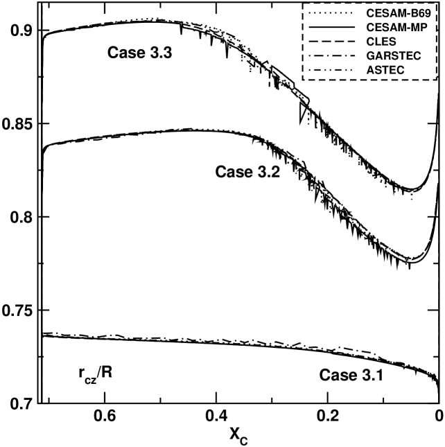
Figure 18: TASK 3: Evolution of the radius of the convective envelope for Cases 3.1, 3.2 and 3.3 (respectively $1.0$, $1.2$ and $1.3$$\,{M}_{\odot}$) in models computed by ASTEC, GARSTEC, CLÉS and CESAM with for the latter two different approaches to treat microscopic diffusion (MP93 and B69)

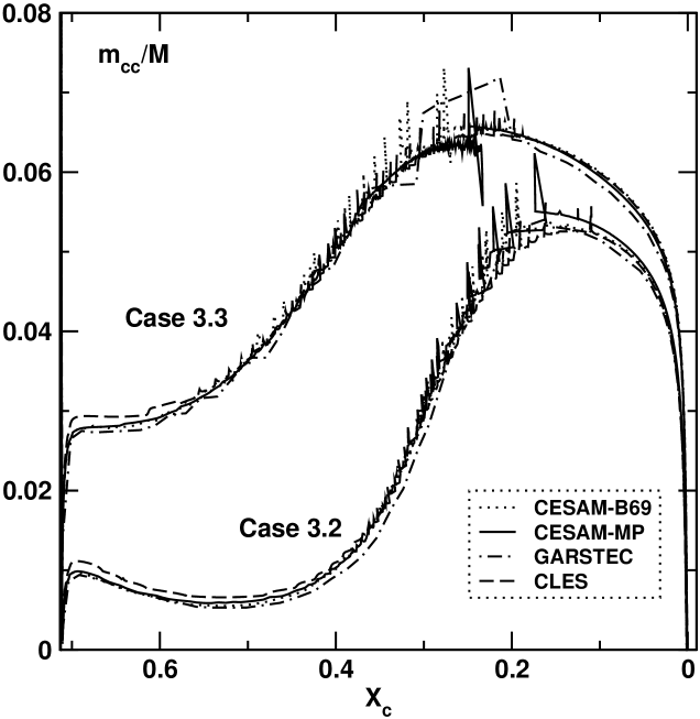
Figure 19: TASK 3: Evolution of the mass of the convective core for Cases 3.2 and 3.3 (respectively $1.0$, $1.2$ and $1.3$$\,{M}_{\odot}$) in models computed by CLÉS, GARSTEC and CESAM with for the latter two different approaches to treat microscopic diffusion (MP93 and B69)

4.2.1 Solar models: Case 3.1

The solar model is characterised by a radiative interior and a convective envelope which deepens as evolution proceeds. The differences in the hydrogen abundance $X$ seen in Fig. 15 can be compared to those found in TASK 1, Case 1.1 model (Fig. 1, top-right). In the centre, where there exists an H gradient built by nuclear reactions and where (in the present case) H is drawn outwards by diffusion, the differences are roughly of the same order of magnitude. In the middle-upper radiative zone, where the settling of He and metals leads to an H enrichment, and in the convection zone, much larger differences are found which reflect different diffusion velocities and also depend on the extension and downward progression of the convective envelope. We note that differences grow with evolution from phase A to C. The sound speed differences reflect differences (i) in the stellar radius, (ii) in the chemical composition gradients in the central regions and below the convective envelope (see the features in the region where $R\in[0.65,0.9]$) and finally (iii) in the location of the convective regions boundaries. They remain quite modest except at the border of the convective envelope and in the zone close to the surface. The differences in $\Gamma_{1}$, seen in the external regions, reflect differences in the He abundance in the regions of second He ionisation. We also note that large differences in luminosity are found on the SGB (phase C).

4.2.2 Solar-type stars with convective cores: Cases 3.2 and 3.3

Those stars of $1.2$ and $1.3$$\,{M}_{\odot}$ have, on the MS, a convective envelope and a convective core. The differences in the hydrogen abundance $X$ seen in the centre in Fig. 16 and 17 are rather similar to those found in TASK 1, Case 1.2 and 1.3 models (Fig. 1, centre and bottom, right). As explained in Sect. 3.4, the core mass is growing during a large fraction of the MS. Due to nuclear reactions a helium gradient builds up at the border of the core. In these regions, the diffusion due to the He concentration gradient competes with the He settling term and finally dominates which makes He move outwards from the core regions. As a consequence metals also diffuse outwards preventing the metal settling. Because of the metal enrichment which induces an opacity increase, the zone at the border of the convective core is the seat of semiconvection (Richard, Michaud, and Richer, 2001).

Also, large differences appear at the bottom of and in the convective envelope in the presence of diffusion. In fact, in these models, diffusion makes the metals pile up beneath the convective envelope which induces an increase of opacity in this zone which in turn triggers convective instability in the form of semiconvection (see Bahcall, Pinsonneault, and Basu, 2001).

4.3 Convection zones

Fig. 18 shows the evolution of the radius of the convective envelope in the models for Cases 3.1, 3.2 and 3.3 while Fig. 19 displays the evolution of the mass of the convective core in Cases 3.2 and 3.3. The crumpled zones in the $r_{\rm cz}/R$ and $m_{\rm cc}/M$ profiles are the signature of the regions of semiconvection which we find for Cases 3.2 and 3.3 either in the regions above the convective core or beneath the convective envelope. As pointed out by Montalbán, Théado, and Lebreton (2007b), in the presence of metal diffusion, it is difficult to study the evolution of the boundaries of convective regions. The numerical treatment of those boundaries in the codes is crucial for the determination of the evolution of the unstable layers: it affects the outer convective zone depths and surface abundances as well as the masses of the convective cores and therefore the evolution of the star.

Rather small differences in the location of the convective boundaries are seen in Figs. 18 and 19. Table 5 displays the properties of the convective zone boundaries. The radii found at the base of the convective envelope in all cases differ by $0.1$–$0.7$ per cent. On the other hand the mass in the convective cores differs by $2$–$4$ per cent except for Case 3.2A where the mass in GARSTEC model differs from the others by more than $10$ per cent.

4.4 Helium surface abundance

Figure 20 displays the helium abundance $Y_{\rm s}$ in the convective envelope for the different cases and phases considered. The evolution of $Y_{\rm s}$ is linked to the efficiency of microscopic diffusion inside the star and to the evolution with time of the internal border of the convective envelope. We note that the surface helium abundance differs by less than $2\%$ for Case 3.1 (any phase) and $3\%$ for Case 3.2 (any phase) and Case 3.3 (phases B and C) whatever the prescription for the diffusion treatment is. For Case 3.3A which is hotter with a thinner convection envelope, the differences between the MP93 prescription for diffusion used in CESAM-MP models and the complete solution of Burger’s equations B69 are rather large. For CESAM-B69 models this difference is of the order of 16%, and a maximum of about $30\%$ in the diffusion efficiency is found between GARSTEC and CESAM-MP. Such differences can indeed be expected and result from the different approaches used to treat microscopic diffusion (MP93 vs. B69) and from the approximations made to calculate the collision integrals. For the solar model, Thoul, Bahcall, and Loeb (1994) found differences of about $15$ per cent between their results – based on the solution of Burger’s equations but with approximations made to estimate the collision integrals- and the MP93 formalism of Michaud and Proffitt (1993) – where the diffusion equations are simplified but in which the collision integrals are obtained according to Paquette et al. (1986). Further tests made by one of us (JM) have shown that for Case 3.2, the use of collision integrals of Paquette et al. (1986) within the formalism by Thoul, Bahcall, and Loeb (1994) leads to differences in the surface He abundance that may amount to $\sim 2.5$ per cent. Since we can expect that the differences of the diffusion coefficients increase as the depth of the convective zone decreases, it is not surprising that in Case 3.3 models differences in the surface helium abundance are even larger. We also point out that the helium depletion is also sensitive to the numerical treatment of convective borders, in particular in the presence of semiconvection.

4.5 Seismic properties

As in Sec. 3.5 we present in Fig. 21 the frequency differences $\nu_{\mbox{\scriptsize CODE}}-\nu_{\mbox{\scriptsize CESAM}}$, where again the frequencies have been scaled to correct for differences in the stellar radius. They can be compared to the results obtained in TASK 1 Cases 1.1, 1.2 and 1.3 (Fig. 10 and 11).

Differences increase as evolution proceeds and as the mass increases. We find that the trend of the differences found in MS models (phase A) for the 3 cases (3.1, 3.2, 3.3) is very similar to what has been found for Case 1.1 and 1.2 MS models. Again the similar behaviour of curves with different degree indicates that the frequency differences are due to near-surface effects. Differences between curves corresponding to modes of degree $\ell=0$ and $1$, which reflect differences in the interior structure, remain small, below $0.1$–$0.2\mu$Hz (a bit larger for ASTEC). The magnitude of the differences is, on the average, higher in models including microscopic diffusion, due to larger differences in the sound speed in particular in the central regions (or border of the convective core) and at the base of the convective envelope. Two different oscillatory components with a periodicity of $\sim 2000$ s and $\sim 4000$ s appear in the frequency differences. The first one which is mainly visible in the GARSTEC models is due to differences in the adiabatic exponent, and its amplitude is related to different helium abundances in the convective envelope. The second one makes the “saw-tooth” profile, and is due to differences at the border of convective envelope.

For TAMS models (phase B), in addition to differences observed for MS models, peaks become clearly visible at low frequencies for $\ell=1$ modes. As in Case 1.3 they can be attributed to differences in the Brunt-Väisälä frequency in the interior and to the mixed character of the corresponding modes. Any difference in the $\mu$ gradient in the region just above the border of the helium core is indeed expected to be seen in the frequency differences. This effect is even larger in SGB models (phase C).

5 Summary and conclusions

We have presented detailed comparisons of the internal structures and seismic properties of stellar models in a range of stellar parameters – mass, chemical composition and evolutionary stage – covering those of the CoRoT targets. The models were calculated by 5 codes (ASTEC, CESAM, CLÉS, STAROX, GARSTEC) which have followed rather closely the specifications for the stellar models (input physics, physical and astronomical constants) that were defined by the ESTA group, although some differences remain, sometimes not fully identified. The oscillation frequencies were calculated by the LOSC code (see Sect. 2.3).

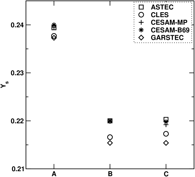
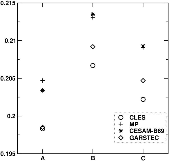
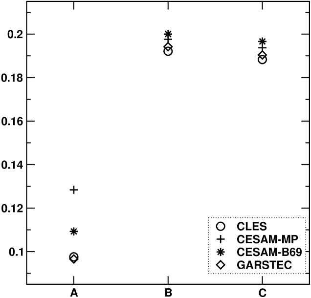
Figure 20: TASK 3: Helium content $Y_{\rm s}$ in the convection envelope for the different codes and cases considered (A and B are for middle and end of the MS respectively while C is for SGB, see Table 2.2) for $1.0$$\,{M}_{\odot}$ (left), $1.2$$\,{M}_{\odot}$ (centre) and $1.3$$\,{M}_{\odot}$ (right).

Figure 21: TASK 3: p-mode frequency differences between models produced by different codes, for Case 3.1 (top row), 3.2 (centre) and 3.3 (bottom). CESAM model is taken as reference, and the frequencies have been scaled to remove the effect of different stellar radii. For each code, we plot two curves corresponding to modes with degrees $\ell=0$ and $\ell=1$.

In a first step, we have examined ESTA-TASK 1 models, calculated for masses in the range $0.9-5$$\,{M}_{\odot}$, with different chemical compositions and evolutionary stages from PMS to SGB. In all these models microscopic diffusion of chemical elements has not been included while one model accounts for overshooting of convective cores. In a second step, we have considered the ESTA-TASK 3 models, in the mass range $1.0-1.3$$\,{M}_{\odot}$, solar composition, and evolutionary stages from the middle of the MS to the SGB. In all these models, microscopic diffusion has been taken into account.

For both tasks we have discussed the maximum and average differences in the physical quantities from centre to surface (hydrogen abundance $X$, pressure $P$, density $\rho$, luminosity $L_{r}$, opacity $\kappa$, adiabatic exponent $\Gamma_{1}$ and gradient $\nabla_{\rm ad}$, specific heat at constant pressure $C_{p}$ and sound speed $c$). We have found that the average differences are in general small. Differences in $P$, $T$, $L_{r}$, $r$, $\rho$ and $\kappa$ are on the percent level while differences in the thermodynamical quantities are often well below $1$%. Concerning the maximal differences, we have found that they are mostly located in the outer layers and in the zones close to the frontiers of the convective zones. As expected, differences generally increase as the evolution proceeds. They are larger in models with convective cores, in particular in models where the convective core increases during a large part of the MS before receding. They are also higher in models including microscopic diffusion or overshooting of the convective core.

Table 11: TASK 3: values of the fractional radius and mass at the base of the convective envelope ($r_{\rm cz}/R$, $m_{\rm cz}/M$ ) and border of the convective core ($r_{\rm cc}/R$, $m_{\rm cc}/M$) and hydrogen abundance in the convection zones

Code	Case	$r_{\rm cz}/R$	$m_{\rm cz}/M$	$X_{\rm cz}$	$r_{\rm cc}/R$	$m_{\rm cc}/M$	$X_{\rm cc}$
ASTEC	3.1A	0.7348	0.9835	0.7436	–	–	–
CESAM-B69	3.1A	0.7326	0.9831	0.7446	–	–	–
CESAM-MP	3.1A	0.7321	0.9830	0.7449	–	–	–
CLÉS	3.1A	0.7315	0.9829	0.7470	–	–	–
GARSTEC	3.1A	0.7357	0.9835	0.7475	–	–	–
ASTEC	3.1B	0.7202	0.9837	0.7630	–	–	–
CESAM-B69	3.1B	0.7153	0.9832	0.7657	–	–	–
CESAM-MP	3.1B	0.7143	0.9830	0.7656	–	–	–
CLÉS	3.1B	0.7151	0.9831	0.7695	–	–	–
GARSTEC	3.1B	0.7159	0.9832	0.7705	–	–	–
ASTEC	3.1C	0.6676	0.9720	0.7627	–	–	–
CESAM-B69	3.1C	0.6644	0.9716	0.7657	–	–	–
CESAM-MP	3.1C	0.6631	0.9713	0.7661	–	–	–
CLÉS	3.1C	0.6643	0.9715	0.7684	–	–	–
GARSTEC	3.1C	0.6643	0.9712	0.7691	–	–	–
ASTEC	3.2A	0.8489	0.9990	0.7754	0.0456	0.0170	0.3500
CESAM-B69	3.2A	0.8451	0.9999	0.7835	0.0451	0.0169	0.3499
CESAM-MP	3.2A	0.8443	0.9990	0.7817	0.0451	0.0170	0.3500
CLÉS	3.2A	0.8444	0.9990	0.7888	0.0447	0.0165	0.3504
GARSTEC	3.2A	0.8450	0.9990	0.7883	0.0433	0.0149	0.3499
CESAM-B69	3.2B	0.7957	0.9969	0.7723	0.0376	0.0325	0.0099
CESAM-MP	3.2B	0.7927	0.9968	0.7723	0.0375	0.0328	0.0100
CLÉS	3.2B	0.7956	0.9969	0.7796	0.0373	0.0319	0.0101
GARSTEC	3.2B	0.7953	0.9969	0.7767	0.0372	0.0318	0.0100
CESAM-B69	3.2C	0.7921	0.9972	0.7768	–	–	–
CESAM-MP	3.2C	0.7913	0.9972	0.7765	–	–	–
CLÉS	3.2C	0.7903	0.9971	0.7843	–	–	–
GARSTEC	3.2C	0.7931	0.9972	0.7814	–	–	–
CESAM-B69	3.3A	0.8916	0.9999	0.8840	0.0641	0.0575	0.3500
CESAM-MP	3.3A	0.8893	0.9998	0.8631	0.0641	0.0572	0.3490
CLÉS	3.3A	0.8893	0.9998	0.8947	0.0633	0.0557	0.3503
GARSTEC	3.3A	0.8920	0.9999	0.8955	0.0631	0.0554	0.3500
CESAM-B69	3.3B	0.8336	0.9990	0.7866	0.0389	0.0404	0.0099
CESAM-MP	3.3B	0.8342	0.9990	0.7886	0.0385	0.0396	0.0100
CLÉS	3.3B	0.8335	0.9990	0.7948	0.0387	0.0399	0.0101
GARSTEC	3.3B	0.8334	0.9989	0.7923	0.0384	0.0391	0.0100
CESAM-B69	3.3C	0.8534	0.9996	0.7902	–	–	–
CESAM-MP	3.3C	0.8517	0.9995	0.7926	–	–	–
CLÉS	3.3C	0.8526	0.9996	0.7988	–	–	–
GARSTEC	3.3C	0.8514	0.9995	0.7963	–	–	–

We have then discussed each case individually and tried to identify the origin of the differences.

The way the codes handle the OPAL-EOS tables has an impact on the output thermodynamical properties of the models. In particular, the choice of the thermodynamical quantities to be taken from the tables and of those to be recalculated from others by means of thermodynamic relations is critical because it is known that some of the thermodynamical quantities tabulated in the OPAL tables are inconsistent (Boothroyd and Sackmann, 2003). In particular, it has been shown by one of us (IW) during one of the ESTA workshops that it is better not to use the tabulated $C_{V}$-value. Some further detailed comparisons of CLÉS and CESAM models by Montalbán et al. (2007a), have demonstrated that these inconsistencies lead to differences in the stellar models and their oscillation frequencies substantially dominating the uncertainties resulting from the use of different interpolation tools. Similarly, the differences in the opacity derived by the codes do not come from the different interpolation schemes but mainly from the differences in the opacity tables themselves. Discrepancies depend on stellar mass and for the cases considered in this study the maximum differences in opacities are of the order of 2% for 2$\,{M}_{\odot}$ models except in a very narrow zone close to $\log T\simeq 4.0$ where there are at a few percents level for all models due to the way the OPAL95 and AF94 tables are combined.

In unevolved models, differences have been found that pertain either to the lack of a detailed calculation of the PMS phase or to the simplifications in the nuclear reactions in the CN cycle. In evolved models we have identified differences which are due to the method used to solve the set of equations governing the temporal evolution of the chemical composition. The shape and position of the $\mu$ gradient and the numerical handling of the temporal evolution of the border of the convection zones are critical as well. The star keeps the memory of the displacements of the convective core (either growing or receding) through the $\mu$ gradient. Models with microscopic diffusion show differences in the He and metals distributions which result from differences in the diffusion velocities and that affect in turn thermodynamic quantities and therefore the oscillation frequencies. The situation is particularly thorny for models that undergo semiconvection, either below the convective zone or at the border of the convective core (for models with diffusion), because none of the codes treats this phenomenon.

We found that differences in the radius at the bottom of the convective envelope are small, lower than $0.7$%. The differences in the mass of the convective core are sometimes large as in models that undergo semiconvection or in PMS and low-mass ZAMS models (up to $17-30$%). In other models, the mass of the convective core differs by $0.5$ to $5$%. Differences in the surface helium abundance in models including microscopic diffusion are of a few per cent except for the $1.3$$\,{M}_{\odot}$ model on the MS where they are in the range $15-30$% due to the different formalisms used to treat diffusion (see Sect. 4).

We have examined the differences in the oscillation frequencies of p and g modes of degrees $\ell=0,1,2,3$. For solar-type stars we also calculated and examined the large frequency separation for $\ell=0,1$ and the frequency separation ratios defined by Roxburgh and Vorontsov (1999).

For solar-type stars on the MS, the differences in the frequencies calculated by the different codes are in the range $0.05-0.1\mu$Hz (for $\ell=0$, no microscopic diffusion) and $0.1-0.2\mu$Hz (models with diffusion). For advanced models (TAMS or SGB) differences are larger (up to $1\mu$Hz for $\ell=0$ modes). We find that the frequency separation ratios are in excellent agreement which confirms that the differences found in the frequencies and in the large frequency separation have their origin in near-surface effects. Differences are larger in models including microscopic diffusion where the sound speed differences are larger (in the centre and at the borders of convection zones). In addition, in evolved models, at low frequency for $\ell=1$ modes, we found differences of up to $4\mu$Hz that result from differences in the Brunt-Väisälä frequency and from the mixed character of the modes. For stars of $2.0$$\,{M}_{\odot}$, frequency differences ($\ell=0,1$ modes) are lower than $0.5\mu$Hz (PMS) and may reach $1\mu$Hz for the evolved model with overshooting. They are due to structure differences in regions close to the surface, in the region of second He-ionisation and close to the centre. In the evolved model some modes are mixed modes sensitive to the location of and features in the $\mu$ gradient. Finally, we found that the frequency differences of the massive models ($3$ and $5$$\,{M}_{\odot}$) are generally smaller than $0.2\mu$Hz.

This thorough comparison work has proven to be very useful in understanding in detail the methods used to handle the calculation of stellar models in different stellar evolution codes. Several bugs and inconsistencies in the codes have been found and corrected. The comparisons have shown that some numerical methods had to be improved and that several simplifications made in the input physics are no longer satisfactory if models of high precision are needed, in particular for asteroseismic applications. We are aware of the weaknesses of the models and therefore of the need for further developments and improvements to bring to them and we are able to give an estimate of the precision they can reach. This gives us confidence on their ability to interpret the asteroseismic observations which are beginning to be delivered by the CoRoT mission where an accuracy of a few $10^{-7}\ {\mathrm{Hz}}$ is expected on the oscillation frequencies (Michel et al., 2006) as well as those that will come from future missions as NASA’s Kepler mission to be launched in 2009 (Christensen-Dalsgaard et al., 2007).