Capacity Bounds for Peak-Constrained Multiantenna Wideband Channels

Abstract

We derive bounds on the noncoherent capacity of a very general class of multiple-input multiple-output channels that allow for selectivity in time and frequency as well as for spatial correlation. The bounds apply to peak-constrained inputs; they are explicit in the channel’s scattering function, are useful for a large range of bandwidth, and allow to coarsely identify the capacity-optimal combination of bandwidth and number of transmit antennas. Furthermore, we obtain a closed-form expression for the first-order Taylor series expansion of capacity in the limit of infinite bandwidth. From this expression, we conclude that in the wideband regime: (i) it is optimal to use only one transmit antenna when the channel is spatially uncorrelated; (ii) rank-one statistical beamforming is optimal if the channel is spatially correlated; and (iii) spatial correlation, be it at the transmitter, the receiver, or both, is beneficial.

I Introduction and Summary of Results

Bandwidth and space are sources of degrees of freedom that can be utilized to transmit information over wireless fading channels. Channel measurements indicate that an increase in the number of degrees of freedom also increases the channel uncertainty that the receiver has to resolve [1]. If the transmit signal is allowed to be peaky, that is, if it can have an unbounded peak value, channel uncertainty is immaterial in the limit of infinite bandwidth. Indeed, for a fairly general class of fading channels, the capacity of the infinite-bandwidth additive white Gaussian noise (AWGN) channel can be achieved [2, 3, 4].

A more realistic modeling assumption is to limit the peak power of the transmitted signal. In this case, the capacity behavior of most channels changes drastically: for certain types of peak constraints, the capacity can even approach zero in the wideband limit [3, 5, 6]. Intuitively, under a peak constraint on the transmit signal, the receiver is no longer able to resolve the channel uncertainty as the number of degrees of freedom increases. Consequently, questions of significant practical relevance are how much bandwidth to use and whether spatial degrees of freedom obtained by multiple antennas can be exploited to increase capacity.

The aim of this paper is to characterize the capacity of spatially correlated multiple-input multiple-output (MIMO) fading channels that are time and frequency selective, i.e., that exhibit memory in frequency and time, given that (i) the transmit signal has bounded peak power and (ii) the transmitter and the receiver know the channel law but both are ignorant of the channel realization. The assumptions (ii) constitute the noncoherent setting, as opposed to the coherent setting where the receiver has perfect channel state information (CSI) and the transmitter knows the channel law only.

Related Work

Sethuraman et al. [7] analyzed the capacity of peak-constrained MIMO Rayleigh-fading channels that are frequency flat, time selective, and spatially uncorrelated and derived an upper bound and a low-SNR lower bound that allow to characterize the second-order Taylor series expansion of capacity around the point $\text{SNR}=0$. In particular, it is shown in [7] that in the low-SNR regime it is optimal to use only a single transmit antenna, while additional receive antennas are always beneficial. The low-SNR results also apply to a wideband channel with fixed total transmit power and increasing bandwidth if the wideband channel can be decomposed into a set of independent and identically distributed (i.i.d.) parallel subchannels in frequency [7].

Spatial correlation is often beneficial in the noncoherent setting. For the separable (Kronecker) spatial correlation model [8, 9], Jafar and Goldsmith [10] proved that transmit correlation increases the capacity of a memoryless fading channel. Moreover, in the low-SNR regime, the rates achievable with on-off keying on memoryless fading channels [11] and with finite-cardinality constellations on block-fading channels [12] increase in the presence of spatial correlation at the transmitter, the receiver, or both.

Contributions

We consider a point-to-point MIMO channel model where each component channel between a given transmit antenna and a given receive antenna is underspread [13] and satisfies the standard wide-sense stationary uncorrelated-scattering (WSSUS) assumption [14]; hence, our channel model allows for selectivity in time and frequency. We assume that the component channels are spatially correlated according to the separable correlation model [8, 9] and that they are characterized by the same scattering function; furthermore, the transmit signal is peak constrained. On the basis of a discrete-time, discrete-frequency approximation of said channel model that is enabled by the underspread property [15], we obtain the following results:

• We derive upper and lower bounds on capacity. These bounds are explicit in the channel’s scattering function and allow to coarsely identify the capacity-optimal combination of bandwidth and number of transmit antennas for a fixed number of receive antennas.

• For spatially uncorrelated channels, we generalize the asymptotic results of Sethuraman et al. [7] to time- and frequency-selective channels: for large enough bandwidth—or equivalently, for small enough SNR—it is optimal to use a single transmit antenna only, while additional receive antennas always increase capacity.

• Differently from the coherent setting [16, 17, 18], we find that both transmit and receive correlation are beneficial in the wideband regime. Furthermore, rank-one statistical beamforming along the strongest eigenmode of the spatial transmit correlation matrix is optimal for large bandwidth.

As the derivations of the results in the present paper rely on several techniques developed in [19] for single-input single-output (SISO) time- and frequency-selective channels, we detail only the new elements in our derivations and refer to [19] otherwise.

Notation

Uppercase boldface letters denote matrices and lowercase boldface letters designate vectors. The superscripts ^T, ^∗, and ^H stand for transposition, element-wise conjugation, and Hermitian transposition, respectively. For two matrices $\mathbf{A}$ and $\mathbf{B}$ of appropriate dimensions, the Hadamard product is denoted as $\mathbf{A}\operatorname{\odot}\mathbf{B}$ and the Kronecker product is denoted as $\mathbf{A}\operatorname{\otimes}\mathbf{B}$; to simplify notation, we use the convention that the ordinary matrix product always precedes the Kronecker and Hadamard products, e.g., $\mathbf{A}\mathbf{B}\operatorname{\odot}\mathbf{C}$ means $(\mathbf{A}\mathbf{B})\operatorname{\odot}\mathbf{C}$ for some matrix $\mathbf{C}$ of appropriate dimension. We designate the identity matrix and the all-zero matrix of dimension $N\times N$ by $\mathbf{I}_{N}$ and $\mathbf{0}_{N}$, respectively; $\mathbf{D}^{1/2}$ is the unique nonnegative definite square-root matrix of the nonnegative definite matrix $\mathbf{D}$. The determinant of a square matrix $\mathbf{X}$ is $\det(\mathbf{X})$, its rank is $\operatorname{rank}(\mathbf{X})$, and its trace is $\operatorname{tr}(\mathbf{X})$. The vector of eigenvalues of $\mathbf{X}$ is denoted by $\bm{\lambda}(\mathbf{X})$, We let $\mathrm{diag}\!\left\{\mathbf{x}\right\}$ denote a diagonal square matrix whose main diagonal contains the elements of the vector $\mathbf{x}$. The function $\delta(x)$ is the Dirac distribution. All logarithms are to the base $e$. For two functions $f(x)$ and $g(x)$, the notation $f(x)=\operatorname{\mathit{o}}\mathopen{}\left(g(x)\right)$ means that $\lim_{x\to 0}f(x)/g(x)=0$. If two random variables $a$ and $b$ follow the same distribution, we write $a\sim b$. Finally, we denote the expectation operator by $\operatorname{\mathbb{E}}\mathopen{}\left[\cdot\right]$ and the Fourier transform operator by $\operatorname{\mathbb{F}}[\cdot]$.

II System Model

In the following subsections, we first introduce the SISO model for one component channel and subsequently discuss the extension of this model to the MIMO setting.

II-A Underspread WSSUS Channels

The relation between the input signal $x(t)$ and the corresponding output signal $y(t)$ of a SISO stochastic linear time-varying (LTV) channel $\operatorname{\mathbb{H}}$ can be expressed as

$$y(t)=\bigl{(}\operatorname{\mathbb{H}}x\bigr{)}(t)+w(t)=\int_{t^{\prime}}k_{\operatorname{\mathbb{H}}}(t,t^{\prime})x(t^{\prime})dt^{\prime}+w(t)$$ (1)

where $k_{\operatorname{\mathbb{H}}}(t,t^{\prime})$ denotes the random kernel of the channel operator $\operatorname{\mathbb{H}}$ and $w(t)$ is a white Gaussian noise process. We assume that $k_{\operatorname{\mathbb{H}}}(t,t^{\prime})$ is a zero-mean jointly proper Gaussian (JPG) process in $t$ and $t^{\prime}$ whose Fourier transforms are well defined. In particular, $L_{\operatorname{\mathbb{H}}}(t,f)=\operatorname{\mathbb{F}}_{\tau\to f}[k_{\operatorname{\mathbb{H}}}(t,t-\tau)]$ is called the time-varying transfer function and $S_{\operatorname{\mathbb{H}}}(\nu,\tau)=\operatorname{\mathbb{F}}_{t\to\nu}[k_{\operatorname{\mathbb{H}}}(t,t-\tau)]$ is called the spreading function. We assume that the channel is WSSUS, so that

$$\operatorname{\mathbb{E}}\mathopen{}\left[S_{\operatorname{\mathbb{H}}}(\nu,\tau)S_{\operatorname{\mathbb{H}}}^{*}(\nu^{\prime},\tau^{\prime})\right]=C_{\operatorname{\mathbb{H}}}(\nu,\tau)\delta(\nu-\nu^{\prime})\delta(\tau-\tau^{\prime}).$$

Consequently, the statistical properties of the channel $\operatorname{\mathbb{H}}$ are completely specified through its so-called scattering function $C_{\operatorname{\mathbb{H}}}(\nu,\tau)$. A WSSUS channel is said to be underspread [15] if $C_{\operatorname{\mathbb{H}}}(\nu,\tau)$ is compactly supported on a rectangle $[-\nu_{0},\nu_{0}]\times[-\tau_{0},\tau_{0}]$ whose spread $\Delta_{\operatorname{\mathbb{H}}}=4\nu_{0}\tau_{0}$ satisfies $\Delta_{\operatorname{\mathbb{H}}}<1$.

II-B Discrete Approximation

To simplify information-theoretic analysis, we would like to diagonalize the channel operator $\operatorname{\mathbb{H}}$, i.e., replace the integral input-output (IO) relation (1) by a countable set of scalar IO relations. To this end, we cannot use an eigendecomposition of the random kernel $k_{\operatorname{\mathbb{H}}}(t,t^{\prime})$ because its eigenfunctions are random as well, and hence unknown to the transmitter and the receiver in the noncoherent setting. Yet, for underspread channels it is possible to find an orthonormal set of deterministic approximate eigenfunctions that depend only on the channel’s scattering function [15]. Consequently, knowledge of the channel law—and hence of the scattering function—is sufficient for transmitter and receiver to approximately diagonalize $\operatorname{\mathbb{H}}$. One possible choice of approximate eigenfunctions is the Weyl-Heisenberg set of mutually orthogonal time-frequency shifts $g_{k,n}(t)=g(t-kT)e^{i2\pi nFt}$ of some prototype function $g(t)$ that is well localized in time and frequency. The grid parameters $T$ and $F$ need to satisfy $TF\geq 1$; then, the kernel of $\operatorname{\mathbb{H}}$ can be approximated as [19]

$$k_{\operatorname{\mathbb{H}}}(t,t^{\prime})\approx\sum_{k=-\infty}^{\infty}\sum_{n=-\infty}^{\infty}\underbrace{L_{\operatorname{\mathbb{H}}}(kT,nF)}_{h[k,n]}g_{k,n}(t)g^{*}_{k,n}(t^{\prime}).$$ (2)

The approximation quality depends on the prototype function $g(t)$ and on the parameters $T$ and $F$, which need to be suitably chosen with respect to the scattering function $C_{\operatorname{\mathbb{H}}}(\nu,\tau)$ [15, 19]. The eigenvalues of the approximate channel with kernel (2) are given by $h[k,n]=L_{\operatorname{\mathbb{H}}}(kT,nF)$. As the channel is JPG and WSSUS, the discretized channel process $\{h[k,n]\}$ is also JPG and stationary in both discrete time $k$ and discrete frequency $n$. We denote its correlation function by $R[k,n]=\operatorname{\mathbb{E}}\mathopen{}\left[h[k^{\prime}+k,n^{\prime}+n]h^{*}[k^{\prime},n^{\prime}]\right]$, normalized as $R[0,0]=1$. The associated spectral density

$$c(\theta,\varphi)=\sum_{k=-\infty}^{\infty}\sum_{n=-\infty}^{\infty}R[k,n]e^{-i2\pi(k\theta-n\varphi)},\quad\left\lvert\theta\right\rvert,\left\lvert\varphi\right\rvert\leq 1/2$$

can be expressed in terms of the scattering function $C_{\operatorname{\mathbb{H}}}(\nu,\tau)$ as [19]

$$c(\theta,\varphi)=\frac{1}{TF}\sum_{k=-\infty}^{\infty}\sum_{n=-\infty}^{\infty}C_{\operatorname{\mathbb{H}}}\mathopen{}\left(\frac{\theta-k}{T},\frac{\varphi-n}{F}\right).$$ (3)

We choose $T\leq 1/(2\nu_{0})$ and $F\leq 1/(2\tau_{0})$ so that no aliasing of the scattering function occurs in (3); for this choice of $T$ and $F$, the normalization $R[0,0]=1$ implies that $\int_{\tau}\!\int_{\nu}{C_{\operatorname{\mathbb{H}}}(\nu,\tau)}d\nu d\tau=1$. Next, we substitute the approximation (2) into (1) and project the input signal $x(t)$ and the output signal $y(t)$ onto the Weyl-Heisenberg set $\{g_{k,n}(t)\}$ to obtain the countable set of scalar IO relations

$$y[k,n]=h[k,n]x[k,n]+w[k,n],$$ (4)

one for each time-frequency slot $(k,n)$. The coefficients $\{w[k,n]\}$ are i.i.d. JPG with zero mean and variance normalized to one.

II-C Extension to Multiple Transmit and Receive Antennas

We extend the SISO channel model in (4) to a MIMO channel model with $M_{T}$ transmit antennas, indexed by $q$, and $M_{R}$ receive antennas, indexed by $r$, and assume that all component channels are characterized by the same scattering function $C_{\operatorname{\mathbb{H}}}(\nu,\tau)$ so that they are diagonalized by the same Weyl-Heisenberg set $\{g_{k,n}(t)\}$. For each slot $(k,n)$ and component channel $(r,q)$ the resulting scalar channel coefficient is denoted as $h_{r,q}[k,n]$. We arrange the coefficients for a given slot $(k,n)$ in an $M_{R}\times M_{T}$ matrix $\bm{\mathsf{H}}[k,n]$ with entries $[\bm{\mathsf{H}}[k,n]]_{r,q}=h_{r,q}[k,n]$. The diagonalized IO relation of the multiantenna channel is then given by a countable set of standard MIMO IO relations of the form

$$\bm{\mathsf{y}}[k,n]=\bm{\mathsf{H}}[k,n]\bm{\mathsf{x}}[k,n]+\bm{\mathsf{w}}[k,n]$$ (5)

where $\bm{\mathsf{x}}[k,n]=\big{[}\begin{matrix}x_{0}[k,n]&x_{1}[k,n]&\cdots&x_{M_{T}-1}[k,n]\end{matrix}\big{]}\raisebox{0.34444pt}{\vphantom{M}}^{T}$ is the $M_{T}$-dimensional input vector for each slot $(k,n)$, $\bm{\mathsf{y}}[k,n]=\big{[}\begin{matrix}y_{0}[k,n]&y_{1}[k,n]&\cdots&y_{M_{R}-1}[k,n]\end{matrix}\big{]}\raisebox{0.34444pt}{\vphantom{M}}^{T}$ is the $M_{R}$-dimensional output vector, and $\bm{\mathsf{w}}[k,n]$ is the $M_{R}$-dimensional noise vector. We allow for spatial correlation according to the separable correlation model [8, 9], so that

$$\operatorname{\mathbb{E}}\mathopen{}\left[h_{r,q}[k^{\prime}+k,n^{\prime}+n]h^{*}_{r^{\prime},q^{\prime}}[k^{\prime},n^{\prime}]\right]=B[r,r^{\prime}]A[q,q^{\prime}]R[k,n].$$

The $M_{T}\times M_{T}$ matrix $\mathbf{A}$ with entries $[\mathbf{A}]_{q,q^{\prime}}=A[q,q^{\prime}]$ is called the transmit correlation matrix, and the $M_{R}\times M_{R}$ matrix $\mathbf{B}$, with entries $[\mathbf{B}]_{r,r^{\prime}}=B[r,r^{\prime}]$, is the receive correlation matrix. Consequently,

$$\bm{\mathsf{H}}[k,n]=\mathbf{B}^{1/2}\bm{\mathsf{H}}_{\mathsf{w}}[k,n](\mathbf{A}^{1/2})^{T}$$ (6)

where $\bm{\mathsf{H}}_{\mathsf{w}}[k,n]$ is an $M_{R}\times M_{T}$ matrix with i.i.d. JPG entries of zero mean and unit variance for all $(k,n)$. We normalize $\mathbf{A}$ and $\mathbf{B}$ so that $\operatorname{tr}(\mathbf{A})=M_{T}$ and $\operatorname{tr}(\mathbf{B})=M_{R}$.

II-D Matrix-Vector Formulation of the Discretized Input-Output Relation

We define a channel use as a $K\times N$ rectangle of time-frequency slots and stack the symbols $\{x_{q}[k,n]\}$ transmitted from all $M_{T}$ transmit antennas during one channel use into an $M_{T}KN$-dimensional vector $\mathbf{x}$, the corresponding output $\{y_{r}[k,n]\}$ for all $M_{R}$ receive antennas into an $M_{R}KN$-dimensional vector $\mathbf{y}$, and likewise the noise $\{w_{r}[k,n]\}$ into an $M_{R}KN$-dimensional vector $\mathbf{w}$. Stacking proceeds first along frequency, then along time, and finally along space, as shown exemplarily for the input vector $\mathbf{x}$:

$$\mathbf{x}_{q}[k] =[x_{q}[k,0]\,x_{q}[k,1]\,\cdots\,x_{q}[k,N-1]]^{T}$$ (7a)

$$\mathbf{x}_{q} =[\mathbf{x}^{T}_{q}[0]\,\mathbf{x}^{T}_{q}[1]\,\cdots\,\mathbf{x}^{T}_{q}[K-1]]^{T}$$ (7b)

$$\mathbf{x} =[\mathbf{x}^{T}_{0}\,\mathbf{x}^{T}_{1}\,\cdots\,\mathbf{x}^{T}_{M_{T}-1}]^{T}.$$ (7c)

Analogously, we stack the channel coefficients, first in frequency to obtain the vectors $\mathbf{h}_{r,q}[k]$, and then in time to obtain a vector $\mathbf{h}_{r,q}$ for each component channel $(r,q)$; further stacking of these vectors along transmit antennas $q$ and then along receive antennas $r$ results in the $M_{T}M_{R}KN$-dimensional vector $\mathbf{h}$. Let $\mathbf{X}_{q}=\mathrm{diag}\!\left\{\mathbf{x}_{q}\right\}$ and $\mathbf{X}=[\mathbf{X}_{0}\,\mathbf{X}_{1}\,\cdots\,\mathbf{X}_{M_{T}-1}]$, where the vectors $\mathbf{x}_{q}$ are defined in (7b). With this notation, the IO relation for one channel use can be conveniently expressed as

$$\mathbf{y}=(\mathbf{I}_{M_{R}}\operatorname{\otimes}\mathbf{X})\mathbf{h}+\mathbf{w}.$$ (8)

The distribution of the channel coefficients in a given channel use is completely characterized by the $M_{T}M_{R}KN\times M_{T}M_{R}KN$ correlation matrix

$$\operatorname{\mathbb{E}}\mathopen{}\left[\mathbf{h}\mathbf{h}^{H}\right]=\mathbf{B}\operatorname{\otimes}\mathbf{A}\operatorname{\otimes}\mathbf{R}$$ (9)

where the correlation matrix $\mathbf{R}=\operatorname{\mathbb{E}}[\mathbf{h}_{r,q}\mathbf{h}^{H}_{r,q}]$ is the same for all component channels $(r,q)$ by assumption; $\mathbf{R}$ is two-level Toeplitz, i.e., block-Toeplitz with Toeplitz blocks. We assume that the three matrices $\mathbf{A}$, $\mathbf{B}$, and $\mathbf{R}$ are known to the transmitter and the receiver.

II-E Power Constraints

We impose a constraint on the average power of the transmitted signal per channel use such that $\operatorname{\mathbb{E}}\mathopen{}\left[\lVert\mathbf{x}\rVert^{2}\right]/T\leq KP$. In addition, we assume a peak constraint across transmit antennas in each slot ($k,n$) according to:

$$\frac{1}{T}\sum_{q=0}^{M_{T}-1}\left\lvert x_{q}[k,n]\right\rvert^{2}\leq\frac{\beta P}{N}$$ (10)

with probability 1 (w.p.1). Here, $\beta\geq 1$ is the peak- to average-power ratio (PAPR).

II-F Spatially Decorrelated Input-Output Relation

Before proceeding to analyze the capacity of the channel just introduced, we make one more cosmetic change to the IO relation (8), which simplifies the exposition of our results considerably. For each slot, we express the input and output vectors in the coordinate systems defined by the eigendecomposition of the transmit and receive correlation matrices, respectively. A similar transformation is used in [10, 12] for a frequency-flat block-fading spatially correlated MIMO channel. Let the eigendecomposition of the spatial correlation matrices be

$$\mathbf{A}=\mathbf{U}_{\!A}\mathbf{\Sigma}\mathbf{U}_{\!A}^{H},\qquad\qquad\mathbf{B} =\mathbf{U}_{\!B}\mathbf{\Lambda}\mathbf{U}_{\!B}^{H},$$

where $\mathbf{\Sigma}=\mathrm{diag}\!\left\{[\sigma_{0}\,\sigma_{1}\,\cdots\,\sigma_{M_{T}-1}]^{T}\right\}$ contains the eigenvalues $\{\sigma_{q}\}$ of $\mathbf{A}$, ordered according to $\sigma_{0}\geq\sigma_{1}\geq\cdots\geq\sigma_{M_{T}-1}$ and, similarly, $\mathbf{\Lambda}=\mathrm{diag}\!\left\{[\lambda_{0}\,\lambda_{1}\,\cdots\,\lambda_{M_{R}-1}]^{T}\right\}$ contains the eigenvalues $\{\lambda_{r}\}$ of $\mathbf{B}$, ordered according to $\lambda_{0}\geq\lambda_{1}\geq\cdots\geq\lambda_{M_{R}-1}$. The columns of $\mathbf{U}_{\!A}$ are called the transmit eigenmodes and the columns of $\mathbf{U}_{\!B}$ are the receive eigenmodes. Instead of the vectors $\bm{\mathsf{x}}[k,n]$ and $\bm{\mathsf{y}}[k,n]$, we use the rotated vectors $\mathbf{U}_{\!A}^{T}\bm{\mathsf{x}}[k,n]$ and $\mathbf{U}_{\!B}^{H}\bm{\mathsf{y}}[k,n]$, respectively, to obtain the following spatially decorrelated IO relation in each slot $(k,n)$:

$$\begin{split}\mathbf{U}_{\!B}^{H}&\bm{\mathsf{y}}[k,n]=\mathbf{U}_{\!B}^{H}\bm{\mathsf{H}}[k,n]\bm{\mathsf{x}}[k,n]+\mathbf{U}_{\!B}^{H}\bm{\mathsf{w}}[k,n]\\ &\stackrel{{\scriptstyle(a)}}{{=}}\mathbf{U}_{\!B}^{H}\bigl{(}\mathbf{U}_{\!B}\mathbf{\Lambda}^{1/2}\mathbf{U}_{\!B}^{H}\bigr{)}\bm{\mathsf{H}}_{\mathsf{w}}[k,n]\bigl{(}\mathbf{U}_{\!A}\mathbf{\Sigma}^{1/2}\mathbf{U}_{\!A}^{H}\bigr{)}^{T}\bm{\mathsf{x}}[k,n]\\ &\hphantom{\stackrel{{\scriptstyle(a)}}{{=}}\mathbf{U}_{\!B}^{H}\bigl{(}\mathbf{U}_{\!B}\mathbf{\Lambda}^{1/2}\mathbf{U}_{\!B}^{H}\bigr{)}\bm{\mathsf{H}}_{\mathsf{w}}[k,n]\mathbf{U}_{\!A}\mathbf{\Sigma}^{1/2}\mathbf{U}_{\!A}^{H}}+\mathbf{U}_{\!B}^{H}\bm{\mathsf{w}}[k,n]\\ &=\mathbf{\Lambda}^{1/2}\mathbf{U}_{\!B}^{H}\bm{\mathsf{H}}_{\mathsf{w}}[k,n]\mathbf{U}_{\!A}^{*}\mathbf{\Sigma}^{1/2}\mathbf{U}_{\!A}^{T}\bm{\mathsf{x}}[k,n]+\mathbf{U}_{\!B}^{H}\bm{\mathsf{w}}[k,n]\end{split}$$ (12)

where (a) follows from (6). Rotations are unitary operations; therefore, $\mathbf{U}_{\!B}^{H}\bm{\mathsf{H}}_{\mathsf{w}}[k,n]\mathbf{U}_{\!A}^{*}\sim\bm{\mathsf{H}}_{\mathsf{w}}[k,n]$ and $\mathbf{U}_{\!B}^{H}\bm{\mathsf{w}}[k,n]\sim\bm{\mathsf{w}}[k,n]$. Furthermore, rotations preserve norms, so that the rotated input vector $\mathbf{U}_{\!A}^{T}\bm{\mathsf{x}}[k,n]$ satisfies the same power constraints as the unrotated input vector $\bm{\mathsf{x}}[k,n]$. Finally, $\mathbf{U}_{\!B}^{H}\bm{\mathsf{y}}[k,n]$ is a sufficient statistic for the output vector $\bm{\mathsf{y}}[k,n]$. These three properties imply that the capacity of the channel with input $\bm{\mathsf{x}}[k,n]$ and output $\bm{\mathsf{y}}[k,n]$ in (5) is the same as the capacity of the spatially decorrelated channel $\mathbf{\Lambda}^{1/2}\bm{\mathsf{H}}_{\mathsf{w}}[k,n]\mathbf{\Sigma}^{1/2}$ in (12) with input $\mathbf{U}_{\!A}^{T}\bm{\mathsf{x}}[k,n]$ and output $\mathbf{U}_{\!B}^{H}\bm{\mathsf{y}}[k,n]$. In the new coordinate system, $q$ indexes transmit eigenmodes instead of transmit antennas, and $r$ indexes receive eigenmodes instead of receive antennas.

It is now tedious but straightforward to similarly rotate the stacked IO relation (8). To keep notation simple, we chose not to introduce new symbols for the rotated input and output and for the spatially decorrelated channel; from here on, all inputs and outputs are with respect to the rotated coordinate systems, and the channel vector $\mathbf{h}$ now stands for the spatially decorrelated stacked channel with correlation matrix

$$\operatorname{\mathbb{E}}\mathopen{}\left[\mathbf{h}\mathbf{h}^{H}\right]=\mathbf{\Lambda}\operatorname{\otimes}\mathbf{\Sigma}\operatorname{\otimes}\mathbf{R}.$$ (13)

This correlation matrix is block diagonal, and hence of much simpler structure than (9).

II-G Advantages and Limitations of the Model

The channel model just presented is fairly general: it allows for correlation in space and for selectivity in time and frequency. Hence, we can dispense with the often used block-fading assumption in time and with the assumption of independent subchannels in frequency. Fortunately, the generality of our model does not come at the price of high modeling complexity as only the scattering function and the spatial correlation matrices $\mathbf{A}$ and $\mathbf{B}$ are needed to describe the distribution of the channel coefficients $\{h_{r,q}[k,n]\}$. Both the scattering function and the spatial correlation matrices can be obtained from channel measurements [20, 21, 9], so that the model can be directly related to real-world channels.

Modeling is synonymous with making assumptions and simplifications. We briefly discuss and justify our key assumptions.

• The assumption that transmitter and receiver do not know the channel realization is accurate, as in a practical system channel realizations can only be inferred from the received signal. The rates achievable with specific methods to obtain CSI, like training schemes, cannot exceed the capacity of the channel in the noncoherent setting.

• Virtually all wireless channels are highly underspread: extremely dispersive outdoor channels with fast moving terminals may have a spread of $\Delta_{\operatorname{\mathbb{H}}}\approx 10^{-2}$, while for slowly varying indoor channels typically $\Delta_{\operatorname{\mathbb{H}}}\approx 10^{-7}$.

• The Weyl-Heisenberg transmission set $\{g_{k,n}(t)\}$ can be interpreted as pulse-shaped (PS) orthogonal frequency-division multiplexing (OFDM); hence, the model we use in our information-theoretic analysis is directly related to a practical transmission scheme.

• We neglect the error incurred by the approximation of the kernel $k_{\operatorname{\mathbb{H}}}(t,t^{\prime})$ in (2), which is equivalent to neglecting intersymbol and intercarrier interference in the corresponding PS-OFDM system interpretation [19]. Yet, if the pulse $g(t)$ and $T$ and $F$ are chosen so as to optimally mitigate intersymbol and intercarrier interference, i.e., if they are matched to the channel’s scattering function [15, 22, 19], we conjecture that the resulting approximation error in (2) is smaller than the corresponding error incurred if either conventional cyclic prefix OFDM or direct sampling of $k_{\operatorname{\mathbb{H}}}(t,t^{\prime})$ and truncation of the resulting sample sequence (e.g., see [5]) is used to analyze underspread WSSUS channels. In fact, these last two decompositions are, in general, not matched to the channel’s scattering function.

• The scattering function models small-scale fading, i.e., the statistical variation of the channel as transmitter, receiver, or objects in the propagation environment are displaced by a few wavelengths [23]. Therefore, if the antennas at each terminal are spaced only a few wavelengths apart, the component channels may be well modeled by the same scattering function.

• We assume that the component channels are spatially correlated according to the separable correlation model [8, 9]. This assumption is common in theoretical analyses of MIMO channels because it greatly simplifies analytical developments. Shortcomings of this model are discussed in [24, 25].

• We assume that spatial correlation does not change over time and frequency. This assumption is valid only over a limited time duration and bandwidth, as it requires the antenna patterns to be constant over frequency and the configuration of dominant scattering clusters to be constant over time.

• The constraint on the peak power across antennas is a reasonable model for a regulatory limit on the total isotropic radiated peak power. If the peak limitation arises from the power amplifiers in the individual transmit chains, a peak constraint per antenna should be used instead.

III Capacity Bounds

With the system model and power constraints in place, we can now proceed to evaluate upper and lower bounds on the capacity of the channel with IO relation (8). Although all results to follow pertain to the channel model described in Section II-D under the power constraints in Section II-E, we use the spatially decorrelated channel and the rotated input and output vectors introduced in Section II-F to simplify the exposition of the proofs.

As we assume that for all $(r,q)$ the process $\{h_{r,q}[k,n]\}$ has a spectral density, given in (3), $\{h_{r,q}[k,n]\}$ is ergodic in $k$ for all component channels [26], and the capacity is given by [27, Chapter 12]

$$C(W)=\lim_{K\rightarrow\infty}\frac{1}{KT}\sup_{\mathcal{P}}I(\mathbf{y};\mathbf{x})$$ (14)

for any fixed bandwidth $W=NF$. The supremum is taken over the set $\mathcal{P}$ of all input distributions that satisfy the constraints on peak and average power in Section II-E.

III-A Upper Bound

Theorem 1

The capacity (14) of the underspread WSSUS MIMO channel in Section II-D under the power constraints in Section II-E is upper-bounded as $C(W)\leq U_{1}(W)$, where

$$U_{1}(W) =$$

$$\sup_{0\leq\alpha\leq\sigma_{0}} \sum_{r=0}^{M_{R}-1}\Biggl{(}\frac{W}{TF}\log\Bigl{(}1+\alpha\lambda_{r}\frac{PTF}{W}\Bigr{)}-\alpha G_{r}(W)\Biggr{)}$$ (15a)

$$G_{r}(W) =\frac{W}{\sigma_{0}\beta}\iint_{\tau\,\nu}\log\mathopen{}\left(1+\frac{\sigma_{0}\lambda_{r}\beta P}{W}C_{\operatorname{\mathbb{H}}}(\nu,\tau)\right)d\nu d\tau.$$ (15b)

Proof:

Let $\mathcal{Q}$ be the set of input distributions that satisfy

$$\frac{1}{T}\operatorname{\mathbb{E}}\mathopen{}\left[\sum_{q=0}^{M_{T}-1}\sigma_{q}\lVert\mathbf{x}_{q}\rVert^{2}\right]\leq\sigma_{0}KP$$ (16)

and the peak constraint (10). As $\sum_{q=0}^{M_{T}-1}\sigma_{q}\operatorname{\mathbb{E}}\mathopen{}\left[\lVert\mathbf{x}_{q}\rVert^{2}\right]\leq\sigma_{0}\sum_{q=0}^{M_{T}-1}\operatorname{\mathbb{E}}\mathopen{}\left[\lVert\mathbf{x}_{q}\rVert^{2}\right]=\sigma_{0}\operatorname{\mathbb{E}}\mathopen{}\left[\lVert\mathbf{x}\rVert^{2}\right]$, any input distribution that satisfies the average-power constraint $\operatorname{\mathbb{E}}\mathopen{}\left[\lVert\mathbf{x}\rVert^{2}\right]/T\leq KP$ also satisfies (16), so that $\mathcal{P}\subset\mathcal{Q}$. To upper-bound $C(W)$, we replace the supremum over $\mathcal{P}$ in (14) with a supremum over $\mathcal{Q}$ and then use the chain rule for mutual information and split the supremum over $\mathcal{Q}$:

$$\sup_{\mathcal{P}}I(\mathbf{y};\mathbf{x})\leq\sup_{\mathcal{Q}}I(\mathbf{y};\mathbf{x})\\ \leq\sup_{0\leq\alpha\leq\sigma_{0}}\Bigl{\{}\sup_{\mathcal{Q}\rvert_{\alpha}}I(\mathbf{y};\mathbf{x},\mathbf{h})-\inf_{\mathcal{Q}\rvert_{\alpha}}I(\mathbf{y};\mathbf{h}\,|\,\mathbf{x})\Bigr{\}}$$ (17)

where the distributions in the restricted set $\mathcal{Q}\rvert_{\alpha}$ satisfy the equality constraint $\operatorname{\mathbb{E}}\bigl{[}\sum_{q=0}^{M_{T}-1}\sigma_{q}\lVert\mathbf{x}_{q}\rVert^{2}\bigr{]}=\alpha KPT$ and the peak constraint (10).

To upper-bound $\sup_{\mathcal{Q}\rvert_{\alpha}}I(\mathbf{y};\mathbf{x},\mathbf{h})$, we drop the peak constraint and take $(\mathbf{I}_{M_{R}}\operatorname{\otimes}\mathbf{X})\mathbf{h}$ as JPG distributed with block-diagonal correlation matrix $\mathbf{\Lambda}\operatorname{\otimes}\operatorname{\mathbb{E}}\mathopen{}\left[\mathbf{X}(\mathbf{\Sigma}\operatorname{\otimes}\mathbf{R})\mathbf{X}^{H}\right]$. Then,

$$\begin{split}I(\mathbf{y};&\mathbf{x},\mathbf{h})\\ &\stackrel{{\scriptstyle(a)}}{{\leq}}\sum_{r=0}^{M_{R}-1}\log\det\Bigl{(}\mathbf{I}_{KN}+\lambda_{r}\sum_{q=0}^{M_{T}-1}\sigma_{q}\operatorname{\mathbb{E}}\mathopen{}\left[\mathbf{x}_{q}\mathbf{x}^{H}_{q}\right]\operatorname{\odot}\mathbf{R}\Bigr{)}\\ &\stackrel{{\scriptstyle(b)}}{{\leq}}\sum_{r=0}^{M_{R}-1}\sum_{n=0}^{N-1}\sum_{k=0}^{K-1}\log\Bigl{(}1+\lambda_{r}\sum_{q=0}^{M_{T}-1}\sigma_{q}\operatorname{\mathbb{E}}\bigl{[}\left\lvert x_{q}[k,n]\right\rvert^{2}\bigr{]}\Bigr{)}\\ &\stackrel{{\scriptstyle(c)}}{{\leq}}KN\sum_{r=0}^{M_{R}-1}\log\mathopen{}\left(1+\frac{\alpha\lambda_{r}PT}{N}\right).\end{split}$$ (18)

Here, (a) follows from the assumption that $(\mathbf{I}_{M_{R}}\operatorname{\otimes}\mathbf{X})\mathbf{h}$ is JPG distributed, from the block diagonal structure of its correlation matrix, and because $\mathbf{X}(\mathbf{\Sigma}\operatorname{\otimes}\mathbf{R})\mathbf{X}^{H}=\sum_{q=0}^{M_{T}-1}\sigma_{q}\mathbf{X}_{q}\mathbf{R}\mathbf{X}_{q}^{H}=\sum_{q=0}^{M_{T}-1}\sigma_{q}\mathbf{x}_{q}\mathbf{x}^{H}_{q}\operatorname{\odot}\mathbf{R}$. Hadamard’s inequality and the normalization $R[0,0]=1$ give (b); finally, (c) follows from Jensen’s inequality.

The derivation of a lower bound on $\inf_{\mathcal{Q}\rvert_{\alpha}}I(\mathbf{y};\mathbf{h}\,|\,\mathbf{x})$ is more involved. Our proof is similar to the proof of the corresponding SISO result in [19, Theorem 1]; therefore, we highlight the novel steps only:

$$\begin{split}\inf_{\mathcal{Q}\rvert_{\alpha}}&I(\mathbf{y};\mathbf{h}\,|\,\mathbf{x})\\ &\stackrel{{\scriptstyle(a)}}{{=}}\inf_{\mathcal{Q}\rvert_{\alpha}}\sum_{r=0}^{M_{R}-1}\operatorname{\mathbb{E}}\mathopen{}\left[\log\det\mathopen{}\left(\mathbf{I}_{KN}+\lambda_{r}\mathbf{X}(\mathbf{\Sigma}\operatorname{\otimes}\mathbf{R})\mathbf{X}^{H}\right)\right]\\ &\stackrel{{\scriptstyle(b)}}{{=}}\inf_{\mathcal{Q}\rvert_{\alpha}}\sum_{r=0}^{M_{R}-1}\operatorname{\mathbb{E}}\Biggl{[}\left(\frac{\log\det\mathopen{}\left(\mathbf{I}_{KN}+\lambda_{r}\mathbf{X}(\mathbf{\Sigma}\operatorname{\otimes}\mathbf{R})\mathbf{X}^{H}\right)}{\sum_{q=0}^{M_{T}-1}\sigma_{q}\lVert\mathbf{x}_{q}\rVert^{2}}\right)\\ &\hphantom{\stackrel{{\scriptstyle(b)}}{{=}}\inf_{\mathcal{Q}\rvert_{\alpha}}\sum_{r=0}^{M_{R}-1}\operatorname{\mathbb{E}}\Biggl{[}}\times\left(\sum_{q=0}^{M_{T}-1}\sigma_{q}\lVert\mathbf{x}_{q}\rVert^{2}\right)\Biggr{]}\\ &\stackrel{{\scriptstyle(c)}}{{\geq}}\sum_{r=0}^{M_{R}-1}\inf_{\mathbf{x}}\frac{\log\det\bigl{(}\mathbf{I}_{KN}+\lambda_{r}\sum_{q=0}^{M_{T}-1}\sigma_{q}\mathbf{x}_{q}\mathbf{x}^{H}_{q}\operatorname{\odot}\mathbf{R}\bigr{)}}{\sum_{q=0}^{M_{T}-1}\sigma_{q}\lVert\mathbf{x}_{q}\rVert^{2}}\\ &\hphantom{\stackrel{{\scriptstyle(b)}}{{=}}\inf_{\mathcal{Q}\rvert_{\alpha}}\sum_{r=0}^{M_{R}-1}\operatorname{\mathbb{E}}\Biggl{[}}\times\inf_{\mathcal{Q}\rvert_{\alpha}}\operatorname{\mathbb{E}}\mathopen{}\left[\sum_{q=0}^{M_{T}-1}\sigma_{q}\lVert\mathbf{x}_{q}\rVert^{2}\right]\\ &\stackrel{{\scriptstyle(d)}}{{\geq}}\alpha KPT\sum_{r=0}^{M_{R}-1}\inf_{\mathbf{x}}\frac{\log\det\bigl{(}\mathbf{I}_{KN}+\lambda_{r}\!\!\sum\limits_{q=0}^{M_{T}-1}\sigma_{q}\mathbf{X}^{H}_{q}\mathbf{X}_{q}\mathbf{R}\bigr{)}}{\sum_{q=0}^{M_{T}-1}\sigma_{q}\lVert\mathbf{x}_{q}\rVert^{2}}\\ &\stackrel{{\scriptstyle(e)}}{{\geq}}\frac{\alpha KTW}{\sigma_{0}\beta}\sum_{r=0}^{M_{R}-1}\iint_{\tau\,\nu}\log\Bigl{(}1+\frac{\sigma_{0}\lambda_{r}\beta P}{W}C_{\operatorname{\mathbb{H}}}(\nu,\tau)\Bigr{)}d\nu d\tau.\end{split}$$

Here, (a) follows from the block-diagonal structure of $\mathbf{\Lambda}\operatorname{\otimes}\mathbf{X}(\mathbf{\Sigma}\operatorname{\otimes}\mathbf{R})\mathbf{X}^{H}$; to obtain (b), we multiply and divide by $\sum_{q=0}^{M_{T}-1}\sigma_{q}\lVert\mathbf{x}_{q}\rVert^{2}$, and to get (c) we replace the first factor in the expectation by its infimum over all input vectors that satisfy the peak constraint (10); (d) follows because $\operatorname{\mathbb{E}}\bigl{[}\sum_{q=0}^{M_{T}-1}\sigma_{q}\lVert\mathbf{x}_{q}\rVert^{2}\bigr{]}=\alpha KPT$ and because $\det(\mathbf{I}_{N}+\mathbf{A}\operatorname{\odot}\mathbf{B})\geq\det(\mathbf{I}_{N}+(\mathbf{I}_{N}\operatorname{\odot}\mathbf{A})\mathbf{B})$ for two $N\times N$ nonnegative definite matrices $\mathbf{A}$ and $\mathbf{B}$—a determinant inequality that we prove in Appendix A; finally, (e) is a consequence [19, Appendix B] of the relation between mutual information and minimum mean square estimation error [28]. To conclude the proof, we note that the bounds on both terms on the right-hand side (RHS) of (17) no longer depend on $K$ upon division by $KT$. ∎

III-A1 The Supremum of $U_{1}(W)$

As the value of $\alpha$ that achieves the supremum in (15a) depends on $W$ in general, the upper bound $U_{1}(W)$ is difficult to interpret. However, for the special case that the supremum is attained for $\alpha=\sigma_{0}$ independently of $W$, the upper bound can be interpreted as the capacity of a set of $M_{R}$ parallel AWGN channels with received power $\sigma_{0}\lambda_{r}P$ and $W/(TF)$ degrees of freedom per second, minus a penalty term that quantifies the capacity loss because of channel uncertainty. We show in Appendix B that a sufficient condition for the supremum in (15a) to be achieved for $\alpha=\sigma_{0}$ is

$$\Delta_{\operatorname{\mathbb{H}}} \leq{\beta}/{(3TF)}$$ (19a)

and

$$0\leq\frac{P}{W} <\frac{\Delta_{\operatorname{\mathbb{H}}}}{\sigma_{0}\lambda_{0}\beta}\left[\exp\mathopen{}\left(\frac{\beta}{2TF\Delta_{\operatorname{\mathbb{H}}}}\right)-1\right].$$ (19b)

As virtually all wireless channels are highly underspread, as $\beta\geq 1$ and, typically, $TF\approx 1.25$, condition (19a) is always satisfied, so that the only relevant condition is (19b); but even for large channel spread, this condition holds for all SNR values $P/W$ of practical interest. As an example, consider a system with $\beta=1$, and $M_{T}=M_{R}=4$ that operates over a channel with spread $\Delta_{\operatorname{\mathbb{H}}}=10^{-2}$. If we use the upper bound $\sigma_{0}\lambda_{0}\leq M_{R}M_{T}$, which follows from the normalization $\operatorname{tr}(\mathbf{A})=M_{T}$ and $\operatorname{tr}(\mathbf{B})=M_{R}$, we find from (19) that $P/W<141\,\mathrm{dB}$ is sufficient for the supremum in (15a) to be achieved for $\alpha=\sigma_{0}$. This value is far in excess of the receive SNR encountered in practical systems. Therefore, we exclusively consider the case $\alpha=\sigma_{0}$ in the remainder of the paper.

III-A2 The Penalty Term

What we call the “penalty term”, i.e., $\sigma_{0}\sum_{r=0}^{M_{R}-1}G_{r}(W)$ in (15), is a lower bound on $\inf_{\mathcal{Q}\rvert_{\alpha}}I(\mathbf{y};\mathbf{h}\,|\,\mathbf{x})$. For SISO channels, it is shown in [19] that of all unit-volume scattering functions with prescribed $\nu_{0}$ and $\tau_{0}$, the brick-shaped scattering function, $C_{\operatorname{\mathbb{H}}}(\nu,\tau)=1/\Delta_{\operatorname{\mathbb{H}}}$ for $(\nu,\tau)\in[-\nu_{0},\nu_{0}]\times[-\tau_{0},\tau_{0}]$, results in the largest penalty term. The same is true for the MIMO channel at hand, where the corresponding capacity is upper-bounded as

$$C(W)\leq\sum_{r=0}^{M_{R}-1}\biggl{\{}\frac{W}{TF}\log\mathopen{}\left(1+\sigma_{0}\lambda_{r}\frac{PTF}{W}\right)\\ -\frac{W\Delta_{\operatorname{\mathbb{H}}}}{\beta}\log\mathopen{}\left(1+\sigma_{0}\lambda_{r}\frac{\beta P}{W\Delta_{\operatorname{\mathbb{H}}}}\right)\biggr{\}}.$$ (20)

The upper bound (20) depends on the channel spread $\Delta_{\operatorname{\mathbb{H}}}$ and the PAPR $\beta$ only through their ratio, so that a decrease in $\Delta_{\operatorname{\mathbb{H}}}$ has the same effect on the upper bound as an increase in the PAPR $\beta$ of the input signal.

III-A3 Spatial Correlation and Number of Antennas

The upper bound $U_{1}(W)$ depends on the transmit correlation matrix $\mathbf{A}$ only through its maximum eigenvalue $\sigma_{0}$, which plays the role of a power gain. This observation shows that rank-one statistical beamforming along any eigenvector of $\mathbf{A}$ corresponding to $\sigma_{0}$ is optimal whenever $U_{1}(W)$ is tight. At high $P/W$ and correspondingly small bandwidth, $U_{1}(W)$ increases linearly in the number of nonzero eigenvalues of the receive correlation matrix, that is, in $\operatorname{rank}(\mathbf{B})$. As the capacity in the coherent setting, which is a simple upper bound on $C(W)$, increases at high $P/W$ linearly only in the minimum of $\operatorname{rank}(\mathbf{A})$ and $\operatorname{rank}(\mathbf{B})$ [17, Proposition 4], we conclude that $U_{1}(W)$ is not tight at high $P/W$. However, for large bandwidth and corresponding small $P/W$, we show in Section IV that $U_{1}(W)$ is tight and that rank-one statistical beamforming is indeed optimal in the wideband regime.

III-B Lower Bound

Theorem 2

Let $\mathbf{C}(\theta)$ denote the $N\times N$ matrix-valued spectral density of an arbitrary component channel $\{\mathbf{h}[k]\}$, i.e.,

$$\mathbf{C}(\theta)=\sum_{k=-\infty}^{\infty}\operatorname{\mathbb{E}}\mathopen{}\left[\mathbf{h}[k^{\prime}+k]\mathbf{h}^{H}[k^{\prime}]\right]e^{-i2\pi k\theta},\quad\left\lvert\theta\right\rvert\leq\frac{1}{2}.$$

Furthermore, let $\bm{\mathsf{s}}$ denote an $M_{T}$-dimensional vector whose first $Q$ elements are i.i.d. and of constant modulus—they have zero mean and satisfy $\left\lvert[\bm{\mathsf{s}}]_{q}\right\rvert^{2}=PT/(QN)$—and let the remaining $M_{T}-Q$ elements be zero. Let $\bm{\mathsf{H}}_{\mathsf{w}}$ be an $M_{R}\times M_{T}$ matrix and let $\bm{\mathsf{w}}$ be an $M_{R}$-dimensional vector, both with i.i.d. JPG entries of zero mean and unit variance. Finally, denote by $I(\bm{\mathsf{y}};\bm{\mathsf{s}}\,|\,\bm{\mathsf{H}}_{\mathsf{w}})$ the coherent mutual information of the memoryless fading MIMO channel with IO relation $\bm{\mathsf{y}}=\mathbf{\Lambda}^{1/2}\bm{\mathsf{H}}_{\mathsf{w}}\mathbf{\Sigma}^{1/2}\bm{\mathsf{s}}+\bm{\mathsf{w}}$. Then, the capacity (14) of the underspread WSSUS MIMO channel in Section II-D under the power constraints in Section II-E is lower-bounded as $C(W)\geq\max_{1\leq Q\leq M_{T}}L_{1}(W,Q)$, where

$$L_{1}(W,Q)=\max_{1\leq\gamma\leq\beta}\Biggl{\{}\frac{W}{\gamma TF}I(\bm{\mathsf{y}};\sqrt{\gamma}\bm{\mathsf{s}}\,|\,\bm{\mathsf{H}}_{\mathsf{w}})\\ -\frac{1}{\gamma T}\sum_{q=0}^{Q-1}\sum_{r=0}^{M_{R}-1}\!\int_{-1/2}^{1/2}\!\!\log\det\mathopen{}\left(\mathbf{I}_{N}+\sigma_{q}\lambda_{r}\frac{\gamma PTF}{QW}\mathbf{C}(\theta)\!\right)\!d\theta\Biggr{\}}.$$ (21)

Proof:

Any specific input distribution leads to a lower bound on capacity; in particular, we choose to transmit constant modulus symbols $x_{q}[k,n]=s_{q}[k,n]$ that are i.i.d. over time, frequency, and eigenmodes, and that satisfy $\left\lvert s_{q}[k,n]\right\rvert^{2}=PT/(QN)$ w.p.1 for all $k,n$ and for $q=0,1,\ldots,Q-1$. The remaining $M_{T}-Q$ eigenmodes are not used to transmit information. We stack the symbols $s_{q}[k,n]$ as in (7) and define the $KN\times M_{T}KN$ matrix

$$\mathbf{S}=\begin{bmatrix}\mathbf{S}_{0}&\mathbf{S}_{1}&\cdots&\mathbf{S}_{Q-1}&\mathbf{0}_{KN}&\cdots&\mathbf{0}_{KN}\end{bmatrix}$$

with $\mathbf{S}_{q}=\mathrm{diag}\!\left\{\mathbf{s}_{q}\right\}$ and where the last $M_{T}-Q$ entries are all-zero matrices $\mathbf{0}_{KN}$. Next, we use

$$I(\mathbf{y};\mathbf{s})\geq I(\mathbf{y};\mathbf{s}\,|\,\mathbf{h})-I(\mathbf{y};\mathbf{h}\,|\,\mathbf{s})$$ (22)

and bound the two terms on the RHS of (22) separately. Because the input is i.i.d., $I(\mathbf{y};\mathbf{s}\,|\,\mathbf{h})=KN\,I(\bm{\mathsf{y}};\bm{\mathsf{s}}\,|\,\bm{\mathsf{H}}_{\mathsf{w}})$. The second term on the RHS of (22) can be evaluated as

$$\begin{split}I(\mathbf{y};\mathbf{h}\,|\,\mathbf{s})&=\sum_{r=0}^{M_{R}-1}\operatorname{\mathbb{E}}\mathopen{}\left[\log\det\mathopen{}\left(\mathbf{I}_{KN}+\lambda_{r}\mathbf{S}(\mathbf{\Sigma}\operatorname{\otimes}\mathbf{R})\mathbf{S}^{H}\right)\right]\\ &\stackrel{{\scriptstyle(a)}}{{\leq}}\sum_{r=0}^{M_{R}-1}\log\det\mathopen{}\left(\mathbf{I}_{QKN}+\lambda_{r}\operatorname{\mathbb{E}}[\mathbf{S}^{H}\mathbf{S}](\mathbf{\Sigma}\operatorname{\otimes}\mathbf{R})\right)\\ &\stackrel{{\scriptstyle(b)}}{{=}}\sum_{q=0}^{Q-1}\sum_{r=0}^{M_{R}-1}\log\det\mathopen{}\left(\mathbf{I}_{KN}+\sigma_{q}\lambda_{r}\frac{PT}{QN}\mathbf{R}\right)\end{split}$$

where (a) follows from Jensen’s inequality because the log-determinant expression is concave in $\mathbf{S}^{H}\mathbf{S}$ [29], and (b) follows because the $\{s_{q}[k,n]\}$ are i.i.d. and have zero mean and constant modulus $\left\lvert s_{q}[k,n]\right\rvert^{2}=PT/(QN)$. We combine the two terms, set $W=NF$, divide by $KT$, and evaluate the limit for $~{}K\to\infty$ by means of [30, Theorem 3.4], a generalization of Szegö’s theorem for multilevel Toeplitz matrices. The resulting lower bound can then be improved upon via time sharing: Let $1\leq\gamma\leq\beta$. We transmit $\sqrt{\gamma}\mathbf{s}$ during a fraction $1/\gamma$ of the transmission time and let the transmitter be silent otherwise. ∎

Wideband Approximation of the Lower Bound

For large enough bandwidth, and hence large enough $N$, the lower bound in Theorem 2 can be well approximated by an expression that is often much easier to evaluate: (i) We replace the first term of $L_{1}(W,Q)$ by its Taylor series expansion up to first order, as given in [31, Theorem 3]. This expansion requires the computation of the expectation of the trace of several terms that involve the channel matrix $\mathbf{\Lambda}^{1/2}\bm{\mathsf{H}}_{\mathsf{w}}\mathbf{\Sigma}^{1/2}$. Lemmas 3 and 4 in [32] provide the desired result. (ii) An approximation of the second term results if we replace the $N\times N$ Toeplitz matrix $\mathbf{C}(\theta)$ by a circulant matrix that is, in $N$, asymptotically equivalent to $\mathbf{C}(\theta)$ [19]. The resulting wideband approximation of $L_{1}(W,Q)$ then reads

$$L_{1}(W,Q)\approx L_{a}(W,Q)=\max_{1\leq\gamma\leq\beta}\Biggl{\{}\frac{M_{R}P}{Q}\sum_{q=0}^{Q-1}\sigma_{q}\\ -\gamma P^{2}\frac{TF}{W}\frac{\left(\sum_{q=0}^{Q-1}\sigma_{q}\right)^{2}\sum_{r=0}^{M_{R}-1}\lambda_{r}^{2}+M_{R}^{2}\sum_{q=0}^{Q-1}\sigma_{q}^{2}}{2Q^{2}}\\ -\frac{W}{\gamma}\sum_{q=0}^{Q-1}\sum_{r=0}^{M_{R}-1}\iint_{\tau\,\nu}\log\left(1+\sigma_{q}\lambda_{r}\frac{\gamma P}{QW}C_{\operatorname{\mathbb{H}}}(\nu,\tau)\right)\!d\nu d\tau\Biggr{\}}.$$ (23)

This approximation is exact for $W\to\infty$ [19].

III-C Numerical Examples

For a $3\times 3$ MIMO system, we show in this section plots of the upper bound $U_{1}(W)$ of Theorem 1, and—for $Q$ between 1 and 3—plots of the lower bound $L_{1}(W,Q)$ of Theorem 2 and of the corresponding approximation $L_{a}(W,Q)$ in (23). The large-bandwidth behavior of the bounds will be substantiated in Section IV.

Numerical Evaluation of the Lower Bound

While the upper bound $U_{1}(W)$ for $\alpha=\sigma_{0}$ can be efficiently evaluated, direct numerical evaluation of the lower bound $L_{1}(W,Q)$ is difficult for large $N$. First, it is necessary to numerically compute the mutual information $I(\bm{\mathsf{y}};\sqrt{\gamma}\bm{\mathsf{s}}\,|\,\bm{\mathsf{H}}_{\mathsf{w}})$ for constant modulus inputs; second, the eigenvalues of the $N\times N$ matrix $\mathbf{C}(\theta)$ are required for the evaluation of the penalty term in (21). While efficient numerical algorithms exist to solve the first task [33], the second task is often challenging, especially if $N$ is large. In [19], we present upper and lower bounds on the penalty term in (21) that are more amenable to numerical evaluation. For the set of parameters considered in the next subsection, these bounds are tight and allow to fully characterize $L_{1}(W,Q)$ numerically.

Parameter Settings

All plots are for a receive power normalized with respect to the noise spectral density of $P/(1\,\mathrm{W}\!/\mathrm{Hz})=1.26\cdot 10^{8}\,\mathrm{s}^{-1}\!$. This parameter value corresponds, for example, to a transmit power of $0.5\,\mathrm{mW}$, a thermal noise level at the receiver of $-174\,\mathrm{dBm}/\mathrm{Hz}$, free-space path loss over a distance of $10\,\mathrm{m}$, and a rather conservative receiver noise figure of $20\,\mathrm{dB}$. Furthermore, we assume that the scattering function is brick shaped with $\tau_{0}=5\,\mathrm{\text{\textmu}s}$, $\nu_{0}=50\,\mathrm{Hz}$, and corresponding spread $\Delta_{\operatorname{\mathbb{H}}}=10^{-3}$. Finally, we set $\beta=1$. For this set of parameter values, we analyze three different scenarios: a spatially uncorrelated channel, spatial correlation at the receiver only, and spatial correlation at the transmitter only.

III-C1 Spatially Uncorrelated Channel

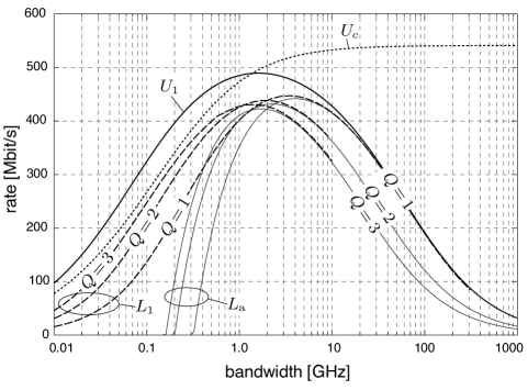
Figure 1: Upper and lower bounds on the capacity of a spatially uncorrelated underspread WSSUS channel with $\mathbf{\Sigma}=\mathbf{\Lambda}=\mathbf{I}_{3}$, $M_{T}=M_{R}=3$, $\beta=1$, and $\Delta_{\operatorname{\mathbb{H}}}=10^{-3}$.

Fig. 1 shows the upper bound $U_{1}(W)$ and—for $Q$ between 1 and 3—the lower bound $L_{1}(W,Q)$ and the corresponding approximation $L_{a}(W,Q)$ for the spatially uncorrelated case $\mathbf{\Sigma}=\mathbf{\Lambda}=\mathbf{I}_{3}$. For comparison, we also plot a standard capacity upper bound $U_{c}(W)$ obtained for the coherent setting and with input subject to an average-power constraint only. We can observe that $U_{c}(W)$ is tighter than $U_{1}(W)$ for small bandwidth; this holds true in general as for small $W$ the penalty term in (15) can be neglected and $U_{1}(W)$ in the spatially uncorrelated case reduces to

$$U_{1}(W)\approx\frac{M_{R}W}{TF}\log\Bigl{(}1+\frac{PTF}{W}\Bigr{)}$$

which is the Jensen upper bound on the capacity $U_{c}(W)$ in the coherent setting. For small and medium bandwidth, the lower bound $L_{1}(W,Q)$ increases with $Q$ and comes surprisingly close to the coherent capacity upper bound $U_{c}(W)$ for $Q=3$.

As can be expected in the light of e.g., [5, 6], when bandwidth increases above a certain critical bandwidth, both $U_{1}(W)$ and $L_{1}(W,Q)$ start to decrease; in this regime, the rate gain resulting from the additional degrees of freedom is offset by the resources required to resolve channel uncertainty. The same argument seems to hold in the wideband regime for the degrees of freedom provided by multiple transmit antennas: $U_{1}(W)$ appears to match $L_{1}(W,Q)$ for $Q=1$; hence, using a single transmit antenna seems optimal in the wideband regime.

III-C2 Impact of Receive Correlation

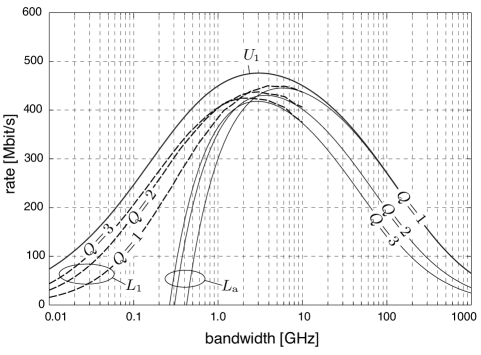
Figure 2: Upper and lower bounds on the capacity of an underspread WSSUS channel that is spatially uncorrelated at the transmitter, $\mathbf{\Sigma}=\mathbf{I}_{3}$, but correlated at the receiver with $\mathbf{\Lambda}=\mathrm{diag}\!\left\{[2.6\>\,0.3\>\,0.1]^{T}\right\}$; $M_{T}=M_{R}=3$, $\beta=1$, and $\Delta_{\operatorname{\mathbb{H}}}=10^{-3}$.

Fig. 2 shows the same bounds as before, but evaluated with spatial correlation $\mathbf{\Lambda}=\mathrm{diag}\!\left\{[2.6\>\,0.3\>\,0.1]^{T}\right\}$ at the receiver and a spatially uncorrelated channel at the transmitter, i.e., $\mathbf{\Sigma}=\mathbf{I}_{3}$. The curves in Fig. 2 are very similar to the ones shown in Fig. 1 for the spatially uncorrelated case, yet they are shifted towards higher bandwidth while the maximum rate is lower. Hence, at least for the example at hand, receive correlation decreases capacity at small bandwidth but it is beneficial at large bandwidth.

III-C3 Impact of Transmit Correlation

We evaluate the same bounds once more, but this time for spatial correlation $\mathbf{\Sigma}=\mathrm{diag}\!\left\{[1.7\>\,1.0\>\,0.3]^{T}\right\}$ at the transmitter and a spatially uncorrelated channel at the receiver, i.e., $\mathbf{\Lambda}=\mathbf{I}_{3}$. The corresponding curves are shown in Fig. 3. Here, transmit correlation increases the capacity at large bandwidth, while its impact at small bandwidth is more difficult to judge because the distance between upper and lower bound increases compared to the spatially uncorrelated case.

All three figures show that for large bandwidth the approximation $L_{a}(W,Q)$ of $L_{1}(W,Q)$ is quite accurate. An observation of significant practical importance is that the bounds $U_{1}(W)$ and $L_{1}(W,Q)$ are quite flat over a large range of bandwidth around their maxima. Further numerical results point at the following: (i) for smaller values of the channel spread $\Delta_{\operatorname{\mathbb{H}}}$, these maxima broaden and extend towards higher bandwidth; (ii) an increase in $\beta$ increases the gap between upper and lower bounds.

IV The Wideband Regime

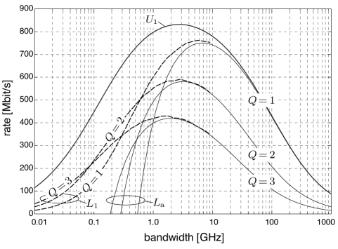
Figure 3: Upper and lower bounds on the capacity of an underspread WSSUS channel that is correlated at the transmitter with $\mathbf{\Sigma}=\mathrm{diag}\!\left\{[1.7\>\,1.0\>\,0.3]^{T}\right\}$ and spatially uncorrelated at the receiver, $\mathbf{\Lambda}=\mathbf{I}_{3}$; $M_{T}=M_{R}=3$, $\beta=1$, and $\Delta_{\operatorname{\mathbb{H}}}=10^{-3}$.

The numerical results in Section III-C suggest that in the wideband regime (i) using a single transmit antenna is optimal when the channel is spatially uncorrelated at the transmitter side; (ii) it is optimal to signal over the maximum transmit eigenmode if transmit correlation is present; (iii) both transmit and receive correlation are beneficial. To substantiate these observations, we compute the first-order Taylor series expansion of $C(W)$ around $1/W=0$.

Theorem 3

Define

$$\kappa_{\operatorname{\mathbb{H}}}=\iint_{\tau\,\nu}C_{\operatorname{\mathbb{H}}}^{2}(\nu,\tau)d\nu d\tau,\qquad\text{and}\qquad\theta=\sum_{r=0}^{M_{R}-1}\lambda_{r}^{2}.$$ (24)

Then, for $\beta>2TF/\kappa_{\operatorname{\mathbb{H}}}$, the capacity (14) of the underspread WSSUS MIMO channel in Section II-D under the power constraints in Section II-E has the following first-order Taylor series expansion around $1/W=0$:

$$C(W)=\frac{a}{W}+\operatorname{\mathit{o}}\mathopen{}\left(\frac{1}{W}\right)$$ (25a)

where

$$a=\theta\,\frac{(\sigma_{0}P)^{2}}{2}\left(\beta\kappa_{\operatorname{\mathbb{H}}}-TF\right).$$ (25b)

Proof:

The proof is a generalization of a similar proof for SISO channels in [19, Appendices E and G]; therefore, we only sketch the main steps.

First, we expand the upper bound in Theorem 1 into a Taylor series. If the channel is highly underspread, the sufficient condition (19) for $\alpha=\sigma_{0}$ to achieve the supremum in (15a) is valid for large enough bandwidth and hence for $W\to\infty$. Therefore, we only need to expand $U_{1}(W)$ for $\alpha=\sigma_{0}$. A more refined analysis in [19, Appendix E] shows that the supremum in (15a) is achieved for $\alpha=\sigma_{0}$ in the large-bandwidth regime if and only if $\beta>2TF/\kappa_{\operatorname{\mathbb{H}}}$, a condition less restrictive than (19a).

It follows from [19, Appendix F] that a Taylor series expansion of the lower bound $L_{1}(W,Q)$ in Theorem 2 does not match the corresponding expansion of $U_{1}(W)$ up to first order, so that we need to devise an alternative, asymptotically tight, lower bound. We observed in Section III-C that signaling over a single transmit eigenmode seems to be optimal for large bandwidth; hence, it is sensible to base the asymptotic lower bound on a signaling scheme that uses only the strongest transmit eigenmode in each slot. In one channel use, we thus transmit $\mathbf{x}=[\mathbf{x}^{T}_{0}\,\mathbf{0}^{T}_{KN}\,\cdots\,\mathbf{0}^{T}_{KN}]^{T}$, where $\mathbf{x}_{0}$ stands for the input vector transmitted on the strongest eigenmode. Such a signaling scheme, often referred to as rank-one statistical beamforming, transmits over all available antennas in general; only if the channel is spatially uncorrelated at the transmitter can antennas be physically switched off. With rank-one statistical beamforming, the spatially decorrelated MIMO channel with IO relation (8) simplifies to a single-input multiple-output (SIMO) channel, the IO relation of which can be conveniently expressed as

$$\tilde{\mathbf{y}}=\tilde{\mathbf{h}}\operatorname{\odot}\tilde{\mathbf{x}}+\tilde{\mathbf{w}}$$

where $\tilde{\mathbf{w}}$ is an $M_{R}KN$-dimensional JPG vector with i.i.d. entries of zero mean and unit variance, the input vector $\tilde{\mathbf{x}}=[\mathbf{x}^{T}_{0}\,\cdots\,\mathbf{x}^{T}_{0}]^{T}$ contains $M_{R}$ copies of $\mathbf{x}_{0}$, and the stacked effective SIMO channel vector is $\tilde{\mathbf{h}}=[\mathbf{h}^{T}_{0,0}\,\mathbf{h}^{T}_{1,0}\,\cdots\,\mathbf{h}^{T}_{M_{R}-1,0}]^{T}$ with correlation matrix $\mathbf{R}_{\tilde{\mathbf{h}}}=\operatorname{\mathbb{E}}\mathopen{}\left[\tilde{\mathbf{h}}\tilde{\mathbf{h}}^{H}\right]=\sigma_{0}\mathbf{\Lambda}\operatorname{\otimes}\mathbf{R}$. The desired asymptotic lower bound now follows directly from the derivation of the asymptotic lower bound for a time-frequency selective SISO channel in [19, Appendix G]. In particular, we choose $\mathbf{x}_{0}$ to be the product of a vector with i.i.d. zero mean constant modulus entries and a nonnegative binary random variable with on-off distribution. Similar signaling schemes were already used in [7] to prove asymptotic capacity results for frequency-flat, time-selective channels. As the first-order Taylor expansion of the resulting lower bound matches the first-order Taylor expansion of $U_{1}(W)$ in (25a), Theorem 3 follows. ∎

Spatial Correlation and Number of Antennas

Rank-one statistical beamforming along any eigenvector of $\mathbf{A}$ associated with $\sigma_{0}$ is optimal to attain the wideband asymptotes of Theorem 3. For channels that are spatially uncorrelated at the transmitter, this result implies that using only one transmit antenna is optimal, as previously shown in [7] for the frequency-flat time-selective case. To further assess the impact of correlation on capacity, we follow [8, 10, 16] and define a partial ordering of correlation matrices through majorization [34]. We say that a correlation matrix $\mathbf{K}$ entails more correlation than a correlation matrix $\mathbf{C}$ if the vector of eigenvalues $\bm{\lambda}(\mathbf{K})$ majorizes $\bm{\lambda}(\mathbf{C})$. To assess the impact of spatial correlation on capacity, we further need the following definition [34]: a scalar function $\phi(\mathbf{z})$ of a vector $\mathbf{z}$ is Schur concave if $\phi(\mathbf{z})\leq\phi(\mathbf{q})$ whenever $\mathbf{z}$ majorizes $\mathbf{q}$.

In the coherent setting, capacity is Schur concave in $\bm{\lambda}(\mathbf{B})$, the eigenvalue vector of the receive correlation matrix while, for sufficiently large bandwidth, it is Schur convex in $\bm{\lambda}(\mathbf{A})$, the eigenvalue vector of the transmit correlation matrix [17, 16]. Hence, in the coherent setting receive correlation is detrimental at any bandwidth while transmit correlation is beneficial at large bandwidth. The intuition is that transmit correlation allows to focus the transmit power into the maximum transmit eigenmode, and the corresponding power gain offsets the reduction in effective transmit signal space dimensions in the power-limited regime, i.e., at large bandwidth. On the other hand, receive correlation is detrimental at any bandwidth because it reduces the effective dimensionality of the receive signal space without any power gain [18].

On the basis of Theorem 3, we conclude that the picture is fundamentally different in the noncoherent setting. The coefficient $a$ in (25) is a Schur-convex function in both the eigenvalue vector $[\sigma_{0}\,\sigma_{1}\,\cdots\,\sigma_{M_{T}-1}]$ of the transmit correlation matrix and the eigenvalue vector $[\lambda_{0}\,\lambda_{1}\,\cdots\,\lambda_{M_{R}-1}]$ of the receive correlation matrix because $\sigma_{0}$ and $\theta$ are continuous convex functions of the corresponding eigenvalue vectors [35]. Hence, both receive and transmit correlation are beneficial for sufficiently large bandwidth. This observation agrees with the results for memoryless and block-fading channels reported in [10, 11, 12]. In the wideband regime, while transmit correlation is beneficial in both the coherent and the noncoherent setting because it allows for power focusing, receive correlation is beneficial rather than detrimental in the noncoherent setting for the following reason: for fixed $M_{T}$ and $M_{R}$, the rate gain obtained from additional bandwidth is offset in the wideband regime by the corresponding increase in channel uncertainty (see Figs. 1, 2, and 3); yet, for fixed but large bandwidth, channel uncertainty decreases in the presence of receive correlation so that capacity increases.

The Lower Bound $L_{1}(W,Q)$ in the Wideband Regime

Since we know that the first-order Taylor expansions around $(1/W)=0$ of the upper bound $U_{1}(W)$ and the lower bound $L_{1}(W,Q)$ do not match, it is surprising that the corresponding curves seem to coincide in Figs. 1, 2, and 3 for large bandwidth. The reason is that, for typical values of $TF$ and $\beta$, the ratio between the first-order coefficients in the Taylor expansions of $L_{1}(W,Q)$ and $C(W)$ approaches 1 as $\kappa_{\operatorname{\mathbb{H}}}$ grows large and $Q=1$. For example, the ratio is $0.998$ for the parameters used in the numerical evaluation in Fig. 1, i.e., $\Delta_{\operatorname{\mathbb{H}}}=10^{-3}$, $\beta=1$, and $TF=1.25$.

V Discussion and Outlook

Capacity analysis in the noncoherent setting is frequently performed asymptotically for either large or small SNR, $P/W$. The corresponding asymptotic results are often useful to obtain design insight, but they may sometimes be misleading: capacity behavior is very sensitive to specific details of the channel model used at high SNR [36], and any channel model eventually breaks down for large enough bandwidth and correspondingly low SNR. The capacity bounds in the present paper are useful for a large range of bandwidth in between these two asymptotic cases (in addition, they are tight in the wideband regime).

The discrete-time discrete-frequency channel model presented in II-B and Section II-C is very general; at the same time, the corresponding capacity bounds in Section III are relatively simple for practically relevant values of $P/W$ and for realistic scattering functions. Furthermore, as our discrete-time discrete-frequency channel model is related to the continuous time WSSUS channel model (1), results from real-world channel measurements can be directly used to obtain capacity estimates. In particular, as the bounds hold for both the regime where degrees of freedom increase capacity, as well as for the regime where degrees of freedom are detrimental, they allow to numerically determine a suitable combination of bandwidth and number of transmit antennas.

For large bandwidth, the bounds are very accurate—the upper bound $U_{1}(W)$ exhibits the correct asymptotic behavior for $W\to\infty$, as shown in Section IV. For small and medium bandwidth, the upper bound $U_{1}(W)$ is not tight, and is indeed worse than the coherent capacity upper bound. The fact that our simple lower bound $L_{1}(W,Q)$ comes quite close to the coherent upper bound $U_{c}(W)$ in Fig. 1 seems to validate, at least for the setting considered, the standard receiver design principle to first estimate the channel and then use the resulting estimates as if they were perfect. To verify this conjecture, though, it is necessary to show that the combination of dedicated channel estimation and coherent signaling achieves rates similar to those predicted by the lower bound $L_{1}(W,Q)$.

The advent of ultrawideband (UWB) communication systems spurred the current interest in wireless communications over channels with very large bandwidth. Current UWB regulations impose a limit on the power spectral density of the transmitted signal, so that the available average power increases with increasing transmission bandwidth. In contrast, we keep the total average transmit power fixed in the present paper; therefore, the results presented here do not directly apply to current UWB regulations. Nonetheless, our bounds allow to assess whether multiple antennas at the transmitter are beneficial for UWB systems. The system parameters used to numerically evaluate the bounds in III-C are compatible with a UWB system that operates over a bandwidth of $7\,\mathrm{GHz}$ and transmits at -41.3 dBm/ MHz. Even if our bounds are not tight at $7\,\mathrm{GHz}$ in this scenario, Figs. 1, 2, and 3 show that the maximum rate increase that can be expected from the use of multiple antennas at the transmitter does not exceed 7%. For channels with smaller spreads than the one in Section III-C, the possible rate increase is even smaller.

Appendix A A Determinant Inequality

Lemma 4

Let $\mathbf{A}$ and $\mathbf{B}$ be two $N\times N$ nonnegative definite Hermitian matrices. Then,

$$\det(\mathbf{I}_{N}+\mathbf{A}\operatorname{\odot}\mathbf{B})\geq\det\bigl{(}\mathbf{I}_{N}+(\mathbf{I}_{N}\operatorname{\odot}\mathbf{A})\mathbf{B}\bigr{)}.$$

Proof:

Assume for now that $\mathbf{A}$ does not have zeros on its main diagonal and define $\tilde{\mathbf{A}}=(\mathbf{I}_{N}\operatorname{\odot}\mathbf{A})^{-1}$. Then,

$$\begin{split}\det(\mathbf{I}_{N}+\mathbf{A}\operatorname{\odot}\mathbf{B})&=\det\bigl{(}\mathbf{A}\operatorname{\odot}(\tilde{\mathbf{A}}+\mathbf{B})\bigr{)}\\ &\stackrel{{\scriptstyle(a)}}{{\geq}}\det(\mathbf{I}_{N}\operatorname{\odot}\mathbf{A})\det(\tilde{\mathbf{A}}+\mathbf{B})\\ &=\det\bigl{(}(\mathbf{I}_{N}\operatorname{\odot}\mathbf{A})\tilde{\mathbf{A}}+(\mathbf{I}_{N}\operatorname{\odot}\mathbf{A})\mathbf{B}\bigr{)}\\ &=\det\bigl{(}\mathbf{I}_{N}+(\mathbf{I}_{N}\operatorname{\odot}\mathbf{A})\mathbf{B}\bigr{)}\end{split}$$ (26)

where (a) is a direct consequence of Oppenheim’s inequality [37, Theorem 7.8.6]. To conclude the proof, we remove the restriction that $\mathbf{A}$ has only nonzero diagonal entries. Because $\mathbf{A}$ is nonnegative definite, its $i$th row and its $i$th column are zero if $[\mathbf{A}]_{ii}=0$ [37, Section 7.1], so that, by the definition of the Hadamard product, the $i$th row and the $i$th column of $\mathbf{A}\operatorname{\odot}\mathbf{B}$ are zero as well. Let $\mathcal{I}$ be the set that contains all indices $i$ for which $[\mathbf{A}]_{ii}=0$, assume without loss of generality that there are $L$ such indices, and let $\mathbf{A}_{\mathcal{I}}$ and $\mathbf{B}_{\mathcal{I}}$ denote the submatrices of $\mathbf{A}$ and $\mathbf{B}$, respectively, with all rows and columns corresponding to $\mathcal{I}$ removed. An expansion by minors of $\det(\mathbf{I}_{N}+\mathbf{A}\operatorname{\odot}\mathbf{B})$ now shows that

$$\det(\mathbf{I}_{N}+\mathbf{A}\operatorname{\odot}\mathbf{B})=\det(\mathbf{I}_{L}+\mathbf{A}_{\mathcal{I}}\operatorname{\odot}\mathbf{B}_{\mathcal{I}}).$$ (27)

Hence, it suffices to apply the inequality (26) to the RHS of (27). ∎

Appendix B Optimization of the Upper Bound

The expression to be maximized in (15a),

$$g(\alpha)=\sum_{r=0}^{M_{R}-1}\Biggl{(}\frac{W}{TF}\log\Bigl{(}1+\alpha\lambda_{r}\frac{PTF}{W}\Bigr{)}-\alpha G_{r}(W)\Biggr{)}$$

where $G_{r}(W)$ is given in (15b), is concave in $\alpha$. Hence, the optimizing parameter $\alpha$ is unique. Furthermore, the following two properties hold: (i) $g(\alpha)=0$for $\alpha=0$. (ii) As, by Jensen’s inequality and because $\log(1+x)\leq x$ $$\begin{split}G_{r}(W)&\leq\frac{W\Delta_{\operatorname{\mathbb{H}}}}{\sigma_{0}\beta}\log\Bigl{(}1+\frac{\sigma_{0}\lambda_{r}\beta P}{W\Delta_{\operatorname{\mathbb{H}}}}\iint_{\tau\,\nu}C_{\operatorname{\mathbb{H}}}(\nu,\tau)d\nu d\tau\Bigr{)}\\ &=\frac{W\Delta_{\operatorname{\mathbb{H}}}}{\sigma_{0}\beta}\log\Bigl{(}1+\frac{\sigma_{0}\lambda_{r}\beta P}{W\Delta_{\operatorname{\mathbb{H}}}}\Bigr{)}\leq\lambda_{r}P,\end{split}$$ (28) the first derivative of $g(\alpha)$,

$$g^{\prime}(\alpha)=\sum_{r=0}^{M_{R}-1}\Bigl{(}\frac{\lambda_{r}P}{1+\alpha\lambda_{r}PTF/W}-G_{r}(W)\Bigr{)}$$ (29)

is nonnegative at $\alpha=0$.

From property (i) and (ii), and from the concavity of $g(\alpha)$, it follows that the supremum in (15a) is achieved for $\alpha=\sigma_{0}$ if and only if the zero of (29) occurs at a point larger or equal to $\sigma_{0}$, or, equivalently, if and only if (29) is positive for $\alpha\in[0,\sigma_{0})$. Identification of this zero-crossing is difficult for $\operatorname{rank}(\mathbf{B})>1$, but we can obtain a sufficient condition for the supremum to be achieved for $\alpha=\sigma_{0}$ as follows:

• The first derivative (29) will certainly be positive if all terms in the sum are positive.

• As for all $\alpha$ in the set $[0,\sigma_{0})$ the inequality

  $$\frac{\lambda_{r}P}{1+\alpha\lambda_{r}PTF/W}\geq\frac{\lambda_{r}P}{1+\sigma_{0}\lambda_{r}PTF/W}$$

  holds, it follows from Jensen’s inequality applied to $G_{r}(W)$ as in (28) that a sufficient condition for the $r$th term in (29) to be positive in $[0,\sigma_{0})$ is

  $$\frac{\lambda_{r}P}{1+\sigma_{0}\lambda_{r}PTF/W}>\frac{W\Delta_{\operatorname{\mathbb{H}}}}{\sigma_{0}\beta}\log\Bigl{(}1+\frac{\sigma_{0}\lambda_{r}\beta P}{W\Delta_{\operatorname{\mathbb{H}}}}\Bigr{)}.$$

• This condition is very similar to one analyzed in [19, Appendix C], and steps identical to the ones detailed in [19, Appendix C] finally lead to (19).

References

- [1] U. G. Schuster and H. Bölcskei, “Ultrawideband channel modeling on the basis of information-theoretic criteria,” IEEE Trans. Wireless Commun., vol. 6, no. 7, pp. 2464–2475, Jul. 2007.
- [2] R. G. Gallager, Information Theory and Reliable Communication. New York, NY, U.S.A.: Wiley, 1968.
- [3] I. E. Telatar and D. N. C. Tse, “Capacity and mutual information of wideband multipath fading channels,” IEEE Trans. Inf. Theory, vol. 46, no. 4, pp. 1384–1400, Jul. 2000.
- [4] G. Durisi, H. Bölcskei, and S. Shamai (Shitz), “Capacity of underspread WSSUS fading channels in the wideband regime,” in Proc. IEEE Int. Symp. Inf. Theory (ISIT), Seattle, WA, U.S.A., Jul. 2006, pp. 1500–1504.
- [5] M. Médard and R. G. Gallager, “Bandwidth scaling for fading multipath channels,” IEEE Trans. Inf. Theory, vol. 48, no. 4, pp. 840–852, Apr. 2002.
- [6] V. G. Subramanian and B. Hajek, “Broad-band fading channels: Signal burstiness and capacity,” IEEE Trans. Inf. Theory, vol. 48, no. 4, pp. 809–827, Apr. 2002.
- [7] V. Sethuraman, L. Wang, B. Hajek, and A. Lapidoth, “Low SNR capacity of noncoherent fading channels,” IEEE Trans. Inf. Theory, 2008, submitted. [Online]. Available: http://arxiv.org/abs/0712.2872
- [8] C.-N. Chuah, D. N. C. Tse, J. M. Kahn, and R. A. Valenzuela, “Capacity scaling in MIMO wireless systems under correlated fading,” IEEE Trans. Inf. Theory, vol. 48, no. 3, pp. 637–650, Mar. 2002.
- [9] J. P. Kermoal, L. Schumacher, K. I. Pedersen, P. E. Mogensen, and F. Frederiksen, “A stochastic MIMO radio channel model with experimental validation,” IEEE J. Sel. Areas Commun., vol. 20, no. 6, pp. 1211–1226, Aug. 2002.
- [10] S. A. Jafar and A. Goldsmith, “Multiple-antenna capacity in correlated Rayleigh fading with channel covariance information,” IEEE Trans. Wireless Commun., vol. 4, no. 3, pp. 990–997, May 2005.
- [11] W. Zhang and J. N. Laneman, “Benefits of spatial correlation for multi-antenna non-coherent communication over fading channels at low SNR,” IEEE Trans. Wireless Commun., vol. 6, no. 3, pp. 887–896, Mar. 2007.
- [12] S. G. Srinivasan and M. K. Varanasi, “Optimal spatial correlation for the noncoherent MIMO Rayleigh fading channel,” IEEE Trans. Wireless Commun., vol. 6, no. 10, pp. 3760–3769, Oct. 2007.
- [13] R. S. Kennedy, Fading Dispersive Communication Channels. New York, NY, U.S.A.: Wiley, 1969.
- [14] P. A. Bello, “Characterization of randomly time-variant linear channels,” IEEE Trans. Commun., vol. 11, no. 4, pp. 360–393, Dec. 1963.
- [15] W. Kozek, “Matched Weyl-Heisenberg expansions of nonstationary environments,” Ph.D. dissertation, Vienna University of Technology, Department of Electrical Engineering, Vienna, Austria, Mar. 1997.
- [16] E. A. Jorswieck and H. Boche, “Performance analysis of MIMO systems in spatially correlated fading using matrix-monotone functions,” IEICE Trans. Fund. Elec. Commun. Comp. Sc., vol. E89-A, no. 5, pp. 1454–1482, May 2006.
- [17] A. M. Tulino, A. Lozano, and S. Verdú, “Impact of antenna correlation on the capacity of multiantenna channels,” IEEE Trans. Inf. Theory, vol. 51, no. 7, pp. 2491–2509, Jul. 2005.
- [18] A. Lozano, A. M. Tulino, and S. Verdú, “Multiantenna capacity: Myths and realities,” in Space-Time Wireless Systems—From Array Processing to MIMO Communications, H. Bölcskei, D. Gesbert, C. B. Papadias, and A.-J. van der Veen, Eds. Cambridge, U.K.: Cambridge Univ. Press, 2006, ch. 5, pp. 87–107.
- [19] G. Durisi, U. G. Schuster, H. Bölcskei, and S. Shamai (Shitz), “Capacity of underspread WSSUS fading channels in the wideband regime under peak constraints,” IEEE Trans. Inf. Theory, 2008, in preparation.
- [20] D. C. Cox, “Delay Doppler characterization of multipath propagation at 910 MHz in a suburban radio environment,” IEEE Trans. Antennas Propag., vol. 20, no. 5, pp. 625–635, Sep. 1972.
- [21] H. Artés, G. Matz, and F. Hlawatsch, “Unbiased scattering function estimators for underspread channels and extension to data-driven operation,” IEEE Trans. Signal Process., vol. 52, no. 5, pp. 1387–1402, May 2004.
- [22] G. Matz, D. Schafhuber, K. Gröchenig, M. Hartmann, and F. Hlawatsch, “Analysis, optimization, and implementation of low-interference wireless multicarrier systems,” IEEE Trans. Wireless Commun., vol. 6, no. 5, pp. 1921–1931, May 2007.
- [23] D. N. C. Tse and P. Viswanath, Fundamentals of Wireless Communication. Cambridge, U.K.: Cambridge Univ. Press, 2005.
- [24] H. Özcelik, M. Herdin, W. Weichselberger, J. Wallace, and E. Bonek, “Deficiencies of ’Kronecker’ MIMO radio channel model,” Electron. Lett., vol. 39, no. 16, pp. 1209–1210, Aug. 2003.
- [25] W. Weichselberger, M. Herdin, H. Özcelik, and E. Bonek, “A stochastic MIMO channel model with joint correlation of both link ends,” IEEE Trans. Wireless Commun., vol. 5, no. 1, pp. 90–100, Jan. 2006.
- [26] G. Maruyama, “The harmonic analysis of stationary stochastic processes,” Memoirs of the Faculty of Science, Kyūshū University, Ser. A, vol. 4, no. 1, pp. 45–106, 1949.
- [27] R. M. Gray, Entropy and Information Theory, revised ed. New York, NY, U.S.A.: Springer, 2007. [Online]. Available: http://ee.stanford.edu/~gray/it.pdf
- [28] D. Guo, S. Shamai (Shitz), and S. Verdú, “Mutual information and minimum mean-square error in Gaussian channels,” IEEE Trans. Inf. Theory, vol. 51, no. 4, pp. 1261–1282, Apr. 2005.
- [29] S. N. Diggavi and T. M. Cover, “The worst additive noise under a covariance constraint,” IEEE Trans. Inf. Theory, vol. 47, no. 7, pp. 3072–3081, Nov. 2001.
- [30] M. Miranda and P. Tilli, “Asymptotic spectra of Hermitian block Toeplitz matrices and preconditioning results,” SIAM J. Matrix Anal. Appl., vol. 21, no. 3, pp. 867–881, Feb. 2000.
- [31] V. V. Prelov and S. Verdú, “Second-order asymptotics of mutual information,” IEEE Trans. Inf. Theory, vol. 50, no. 8, pp. 1567–1580, Aug. 2004.
- [32] A. Lozano, A. M. Tulino, and S. Verdú, “Multiple-antenna capacity in the low-power regime,” IEEE Trans. Inf. Theory, vol. 49, no. 10, pp. 2527–2544, Oct. 2003.
- [33] W. He and C. N. Georghiades, “Computing the capacity of a MIMO fading channel under PSK signaling,” IEEE Trans. Inf. Theory, vol. 51, no. 5, pp. 1794–1803, May 2005.
- [34] A. W. Marshall and I. Olkin, Inequalities: Theory of Majorization and Its Applications. New York, NY, U.S.A.: Academic Press, 1979.
- [35] A. W. Marshall and F. Proschan, “An inequality for convex functions involving majorization,” J. Math. Anal. Appl., vol. 12, no. 1, pp. 87–90, Aug. 1965.
- [36] A. Lapidoth, “On the asymptotic capacity of stationary Gaussian fading channels,” IEEE Trans. Inf. Theory, vol. 51, no. 2, pp. 437–446, Feb. 2005.
- [37] R. A. Horn and C. R. Johnson, Matrix Analysis. Cambridge, U.K.: Cambridge Univ. Press, 1985.