Detecting rigid convexity of
bivariate polynomials

Abstract

Given a polynomial $x\in{\mathbb{R}}^{n}\mapsto p(x)$ in $n=2$ variables, a symbolic-numerical algorithm is first described for detecting whether the connected component of the plane sublevel set ${\mathcal{P}}=\{x:p(x)\geq 0\}$ containing the origin is rigidly convex, or equivalently, whether it has a linear matrix inequality (LMI) representation, or equivalently, if polynomial $p(x)$ is hyperbolic with respect to the origin. The problem boils down to checking whether a univariate polynomial matrix is positive semidefinite, an optimization problem that can be solved with eigenvalue decomposition. When the variety ${\mathcal{C}}=\{x:p(x)=0\}$ is an algebraic curve of genus zero, a second algorithm based on Bézoutians is proposed to detect whether $\mathcal{P}$ has an LMI representation and to build such a representation from a rational parametrization of $\mathcal{C}$. Finally, some extensions to positive genus curves and to the case $n>2$ are mentioned.

Keywords
Polynomial, convexity, linear matrix inequality, real algebraic geometry.

1 Introduction

Linear matrix inequalities (LMIs) are versatile modeling objects in the context of convex programming, with many engineering applications [5]. An $n$-dimensional LMI set is defined as

$${\mathcal{F}}=\{x\in{\mathbb{R}}^{n}\>:\>F(x)=F_{0}+\sum_{i=1}^{n}x_{i}F_{i}\succeq 0\}$$ (1)

where the $F_{i}\in{\mathbb{R}}^{m\times m}$ are given symmetric matrices of size $m$ and $\succeq 0$ means positive semidefinite. From the characteristic polynomial

$$t\mapsto\det(tI_{m}+F(x))=p_{0}(x)+p_{1}(x)t+\cdots+p_{m-1}(x)t^{m}+t^{m}$$

it follows from e.g. [36, Theorem 20] that

$${\mathcal{F}}=\{x\in{\mathbb{R}}^{n}\>:\>p_{0}(x)\geq 0,\ldots,p_{m-1}(x)\geq 0\}.$$ (2)

Hence the LMI set $\mathcal{F}$ is basic semialgebraic: it is the intersection of polynomial sublevel sets. From linearity of $F(x)$ and convexity of the cone of positive semidefinite matrices, it also follows that $\mathcal{F}$ is convex. Hence LMI sets are convex basic semialgebraic.

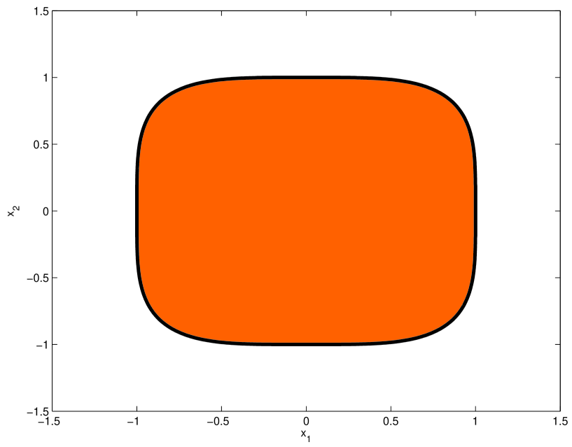
Figure 1: The TV screen level set is not LMI.

One may then wonder whether all convex basic semialgebraic sets are LMI. In [23], Helton and Vinnikov answer by the negative, showing that in the plane ($n=2$) some convex basic semialgebraic sets cannot be LMI. An elementary example is the so-called TV screen set defined by the Fermat quartic

$$\{x\in{\mathbb{R}}^{2}\>:\>1-x_{1}^{4}-x_{2}^{4}\geq 0\}$$ (3)

see Figure 1.

1.1 Rigid convexity

Assume that the set $\mathcal{F}$ defined in (1) has a non-empty interior, and choose a point $x_{0}$ in this interior, i.e.

$$x_{0}\in\mathrm{int}\>{\mathcal{F}}=\{x\>:\>F(x)\succ 0\}$$

where $\succ 0$ means positive definite. A segment starting from $x_{0}$ attains the boundary of $\mathcal{F}$ when the determinant $p_{0}(x)=\mathrm{det}\>F(x)$ vanishes. The remaining polynomial inequalities $p_{i}(x)\geq 0$, $i>0$ only isolate the convex connected component containing $x_{0}$. This motivated Helton and Vinnikov [23] to study semialgebraic sets defined by a single polynomial inequality

$${\mathcal{P}}=\{x\in{\mathbb{R}}^{n}\>:\>p(x)\geq 0\}.$$ (4)

The set $\{x\>:\>p(x)>0\}$ is called an algebraic interior with defining polynomial $p(x)$, and it is equal to $\mathrm{int}\>{\mathcal{P}}$ when $\mathcal{P}$ is convex. With these notations, the question addressed in [23] is as follows: what are the conditions satisfied by a polynomial $p(x)$ so that $\mathcal{P}$ is an LMI set ?

For notational simplicity we will assume, without loss of generality, that $x_{0}=0$, so that $\mathcal{P}$ contains the origin, and hence we can normalize $p(x)$ so that $p(0)=1$.

If $p(x)=\mathrm{det}\>F(x)$ for some matrix mapping $F(x)$ we say that $p(x)$ has a determinantal representation. In particular, the polynomial $p_{0}(x)$ in (2) has a symmetric linear determinantal representation.

Consider an LMI set $\mathcal{F}$ as in (1) and define

$$p(x)=\det F(x)$$

as the determinant of the symmetric pencil $F(x)$. Note that $\deg p=m$, the dimension of $F(x)$. Define the algebraic variety

$${\mathcal{C}}=\{x\in{\mathbb{R}}^{n}\>:\>p(x)=0\}$$ (5)

and notice that the boundary of $\mathcal{F}$ is included in $\mathcal{C}$. Indeed, a point $x^{*}$ along the boundary of $\mathcal{F}$ is such that the rank of $F(x^{*})$ vanishes. Since the origin belongs to $\mathcal{F}$ it holds $F_{0}\succeq 0$.

Now consider a line passing through the origin, parametrized as $x(t,z)=tz$ where $t\in\mathbb{R}$ is a parameter and $z\in{\mathbb{R}}^{n}$ is any vector with unit norm. For all $z$, the symmetric matrix $F(x(t,z))=F_{0}+t(z_{1}F_{1}+\cdots+z_{n}F_{n})$ has only real eigenvalues as a pencil of $t$, and its determinant $t\mapsto p(x(t,z))=\det F(x(t))$ has only real roots. Therefore, a given polynomial level set $\mathcal{P}$ as in (4) is LMI only if the polynomial $t\mapsto p(x(t,z))$ has only real roots for all $z$, it must satisfy the so-called real zero condition [23]. Geometrically it means that a generic line passing through the origin must intersect the variety (5) at $m=\deg p$ real points. The set $\mathcal{P}$ is then called rigidly convex, a geometric property implying convexity.

A striking result of [23] is that rigid convexity is also a sufficient condition for a polynomial level set to be an LMI set in the plane, i.e. when $n=2$. For example, it can be checked easily that the TV screen set (3) is not rigidly convex since a generic line cuts the quartic curve only twice.

In the litterature on partial differential equations, polynomials satisfying real zero condition are also called hyperbolic polynomials, and the corresponding LMI set is called the hyperbolicity cone, see [36] for a survey, and [31] for connections between real zero and hyperbolic polynomials.

In passing, note the fundamental distinction between an LMI set (as defined above) and a semidefinite representable set, as defined in [33, 5]. A semidefinite representable set is the projection of an LMI set:

$${\mathcal{F}}=\{x\in{\mathbb{R}}^{n}\>:\>\exists u\in{\mathbb{R}}^{n_{u}}\>:\>F(x,u)=F_{0}+\sum_{i=1}^{n}x_{i}F_{i}+\sum_{j=1}^{n_{u}}u_{j}G_{j}\succeq 0\}$$

where the variables $u_{j}$, sometimes called liftings, are instrumental to the construction of the set through an extended pencil $F(x,u)$. Such a set is called a lifted LMI set. It is convex semialgebraic, but in general it is not basic. However, it can be expressed as a union of basic semialgebraic sets. In the case of the TV screen set (3) a lifted LMI representation follows from the extended pencil

$$F(x,u)=\left[\begin{array}[]{cccccc}1+u_{1}&u_{2}\\ u_{2}&1-u_{1}\\ &&1&x_{1}\\ &&x_{1}&u_{1}\\ &&&&1&x_{2}\\ &&&&x_{2}&u_{2}\end{array}\right]$$

obtained by introducing two liftings. It seems that the problem of knowing which convex semialgebraic sets are semidefinite representable is still mostly open, see [30, 24] for recent developments.

1.2 Determinantal representation

Once rigid convexity of a plane set, or equivalently the real zero property of its defining polynomial, is established, the next step is constructing an LMI representation. Algebraically, given a real zero bivariate polynomial $p(x_{1},x_{2})$ of degree $m$, the problem consists in finding symmetric matrices $F_{0}$, $F_{1}$ and $F_{2}$ of dimension $m$ such that

$$p(x_{1},x_{2})=\det(F_{0}+F_{1}x_{1}+F_{2}x_{2})$$

and $F_{0}\succeq 0$. If the $F_{i}$ are symmetric complex-valued matrices, this is a well-studied problem of algebraic geometry called determinantal representation, see [37] for a classical reference and [3, 34] for more recent surveys and extensions to trivariate polynomials.

If one relaxes the dimension constraint (allowing the $F_{i}$ to have dimension larger than $m$) and the symmetry constraint (allowing the $F_{i}$ to be non-symmetric), then results from linear systems state-space realization theory (in particular linear fractional representations, LFRs) can be invoked to design computer algorithms solving constructively the determinantal representation problem. For example, the LFR toolbox for Matlab [21] is a user-friendly package allowing to find non-symmetric determinantal representations:

>> lfrs x1 x2
>> f=1/(1-x1^4-x2^4)
..
LFR-object with 1 output(s), 1 input(s) and 0 state(s).
Uncertainty blocks (globally (8 x 8)):
 Name  Dims  Type   Real/Cplx   Full/Scal   Bounds
 x1    4x4   LTI       r           s        [-1,1]
 x2    4x4   LTI       r           s        [-1,1]

The software builds a state-space realization of order 8 of the transfer function $f(x)=1/p(x)$. This indicates that a non-symmetric real pencil $F(x)$ of dimension 8 could be found that satisfies $\det F(x)=p(x)$, as evidenced by the following script using the Symbolic Math Toolbox (Matlab gateway to Maple):

>> syms x1 x2
>> D=diag([ones(1,4)*x1 ones(1,4)*x2]);
>> F=eye(8)-F.a*D
F =
[   1, -x1,   0,   0,   0,   0,   0,   0]
[   0,   1, -x1,   0,   0,   0,   0,   0]
[   0,   0,   1, -x1,   0,   0,   0,   0]
[ -x1,   0,   0,   1, -x2,   0,   0,   0]
[   0,   0,   0,   0,   1, -x2,   0,   0]
[   0,   0,   0,   0,   0,   1, -x2,   0]
[   0,   0,   0,   0,   0,   0,   1, -x2]
[ -x1,   0,   0,   0, -x2,   0,   0,   1]
>> det(F)
ans =
-x2^4+1-x1^4

Note that LFR and state-space realization techniques are not restricted to the bivariate case, but they result in pencils of large dimension (typically much larger than the degree of the polynomial), and there is apparently no easy way to reduce the size of a pencil.

If one insists on having the $F_{i}$ symmetric, then results from non-commutative state-space realizations can be invoked to derive a determinantal representation, at the price of relaxing the sign constraint on $F_{0}$. An implementation is available in the NC Mathematica package [22]. Here too, these techniques may produce pencils of large dimension.

Now if one insists on having symmetric $F_{i}$ of minimal dimension $m$, then two essentially equivalent constructive procedures are known in the bivariate case to derive Hermitian complex-valued $F_{i}$ from a defining polynomial $p(x_{1},x_{2})$ of degree $m$. Real symmetric solutions must then be extracted from the set of complex Hermitian solutions.

The first one is based on the construction of a basis for the Riemann-Roch space of complete linear systems of the algebraic plane curve $\mathcal{C}$ given in (5). The procedure is described in [12]: one needs to find a curve of degree $m-1$ touching $\mathcal{C}$ at each intersection point, i.e. the gradients must match. The algorithm is illustrated in [32]. It is not clear however how to build a touching curve ensuring $F_{0}\succeq 0$.

The second determinantal representation algorithm is sketched in [23] and in much more detail in [45]. It is based on complex Riemann surface theory [20, 16]. Explicit expressions for the $F_{i}$ matrices are given via theta functions. Numerically, the key ingredient is the computation of the period matrix of the algebraic curve and the corresponding Abel-Jacobi map. The period matrix of a curve can be computed numerically with the algcurves package of Maple, see [11] and the tutorial [10] for recent developments, including new algorithms for explicit computations of the Abel-Jacobi map. A working computer implementation taking $p(x_{1},x_{2})$ as input and producing the $F_{i}$ matrices as output is still missing however.

1.3 Contribution

The focus of this paper is mostly on computational methods and numerical algorithms. The contribution is twofold.

First in Section 2 we describe an algorithm for detecting rigid convexity in the plane. Given a bivariate polynomial $p(x_{1},x_{2})$, the algorithm uses a hybrid symbolic-numerical method to detect whether the connected component of the sublevel set (4) containing the origin is rigidly convex. The problem boils down to deciding whether a univariate polynomial matrix is positive semidefinite. This is a well-known problem in linear systems theory, for which numerical linear algebra algorithms are available (namely eigenvalue decomposition), as well as a (more expensive but more flexible) semidefinite programming formulation.

Then in Section 3 we describe an algorithm for solving the determinantal representation problem for algebraic plane curves of genus zero. The algorithm is essentially symbolic, using Bézoutians, but it assumes that a rational parametrization of the curve is available. The idea behind the algorithm is not new, and can be traced back to [28], as surveyed recently in [27]. An algorithm for detecting rigid convexity of a connected component delimited by such curves readily follows.

Extensions to positive genus algebraic plane curves and higher dimensional sets are mentioned in Section 4. In particular we survey the case of cubic plane curves and cubic surfaces which are well understood. The case of quartic (and higher degree) curves seems to be mostly open, and computer implementations of determinantal representations are still missing. Similarly, checking rigid convexity in higher dimensions seems to be computational challenging since it amounts to deciding whether a multivariate polynomial matrix is positive semidefinite.

2 Detecting rigid convexity in the plane

In this section we design an algorithm to assess whether the connected component delimited by a bivariate polynomial around the origin is rigidly convex. The idea is elementary and consists in formulating algebraically the geometric condition of rigid convexity of the set $\mathcal{P}$ defined in (4): a line passing through the origin cuts the algebraic curve $\mathcal{C}$ defined in (5) a number of times which is equal to the total degree $m$ of the defining bivariate polynomial

$$x\in{\mathbb{R}}^{2}\mapsto p(x)=\sum_{\alpha\in{\mathbb{N}}^{2},|\alpha|\leq m}p_{\alpha}x^{\alpha}=p_{00}+p_{10}x_{1}+p_{01}x_{2}+p_{20}x_{1}^{2}+p_{11}x_{1}x_{2}+\cdots$$

A line passing through the origin can be parametrized as:

$$\begin{array}[]{rcl}x_{1}&=&r\cos\theta=t^{-1}(z^{-1}+z)\\ x_{2}&=&r\sin\theta=it^{-1}(z^{-1}-z)\end{array}$$ (6)

where $z=e^{i\theta}$ and $t=2r^{-1}$. Along this line, we define

$$t\in{\mathbb{R}}\mapsto q(t)=t^{m}p(x)=\sum_{k=0}^{m}q_{k}(z)t^{k}$$ (7)

as a univariate polynomial of degree $m$ which vanishes on $\mathcal{C}$. Moreover $q(t)$ is monic since $q_{m}(z)=p(0)=1$. The remaining coefficients are Laurent polynomials

$$q_{\beta}(z)=\sum_{k=0}^{m}q_{\beta k}(z^{k}+z^{-k})$$

with real coefficients, also called trigonometric cosine polynomials. Set $\mathcal{P}$ is rigidly convex if and only if this polynomial has only real roots, i.e. if the number of intersections of the line with the curve $\mathcal{C}$ is maximal.

2.1 Counting the real roots of a polynomial

A well-known result of real algebraic geometry [2, Theorem 4.57] states that a univariate polynomial $q(t)$ of degree $m$ has only real roots if and only if its Hermite matrix is positive semidefinite. The Hermite matrix is the $m$-by-$m$ moment matrix of a discrete measure supported with unit weights on the roots $x_{1},\ldots,x_{m}$ of polynomial $q(t)$ (note that these roots are not necessarily distinct). It is a symmetric Hankel matrix whose entries $(i,j)$ are Newton sums $N_{i+j}=\sum_{k=1}^{m}x_{k}^{i+j}$. The Newton sums are elementary symmetric functions of the roots that can be expressed explicitly as polynomial functions of the coefficients of $q(t)$. Recursive expressions are available to compute the $N_{k}$, or equivalently, $N_{k}=\mathrm{trace}\>C^{k}$ where $C$ is a companion matrix of polynomial $q(t)$, i.e. a matrix with eigenvalues $x_{i}$, see e.g. [2, Proposition 4.54]. Recall that coefficients of the polynomial $q(t)$ given in (7) are Laurent polynomials. It follows that the Hermite matrix of $q(t)$ is a symmetric trigonometric polynomial matrix of dimension $m$, that we denote by $H(z)$. We have proved the following result.

Lemma 1

The bivariate polynomial $p(x)$ is rigidly convex if and only if its Hermite matrix $H(z)$ is positive semidefinite along the unit circle. Coefficients of $H(z)$ are explicit polynomial expressions of the coefficients of $p(x)$.

2.2 Positive semidefiniteness of polynomial matrices

The problem of checking positive semidefiniteness of a polynomial matrix on the unit circle is generally referred to as (discrete-time) spectral factorization. It is a well-known problem of systems and circuit theory [47, 46, 19]. The positivity condition can also be defined on the imaginary axis (continuous-time spectral factorization) or the real axis. Various numerical methods are available to solve this problem [29]. Several algorithms are implemented in the Polynomial Toolbox for Matlab [35]. In increasing order of complexity, we can distinguish between

• Newton-Raphson algorithms: the spectral factorization problem is formulated as a quadratic polynomial matrix equation which is then solved iteratively [26]. At each step, a linear polynomial matrix equation must be solved [25]. Quadratic (resp. linear) convergence is ensured locally if the polynomial matrix is positive definite (resp. semidefinite);

• polynomial operations: a sequence of elementary operations is carried out in the ring of polynomials to reduce the polynomial matrix to some canonical form, see [8] and [48] for a recent survey. These algorithms are cheap computationally but their numerical behavior (stability) is unclear;

• algebraic Riccati equation: using state-space realization, the problem is formulated as a quadratic matrix equation, which in turn can be solved via a matrix eigenvalue decomposition with a particular structure [46, 19, 41];

• semidefinite programming: polynomial matrix positivity is formulated as a convex semidefinite program, see [41] and the recent surveys [17, 18]. The particular structure of this semidefinite program can be exploited in interior-point schemes, in particular when forming the gradient and Hessian. General purpose semidefinite solvers can be used as well.

The semidefinite programming formulation of discrete-time polynomial matrix factorization, a straightfoward transposition of the continuous-time case studied in [41], is as follows. The symmetric trigonometric polynomial matrix $H(z)=H_{0}+H_{1}(z+z^{-1})+\cdots+H_{d}(z^{d}+z^{-d})$ of size $m$ is positive semidefinite along the unit circle if and only if there is a symmetric matrix $P$ of size $dm$ such that

$$\begin{array}[]{rcl}L(P)&=&\left[\begin{array}[]{c|ccc}H_{0}&H_{1}&\cdots&H_{d}\\ \hline\cr H_{1}&0&&0\\ \vdots&&\ddots\\ H_{d}&0&\cdots&0\end{array}\right]+\left[\begin{array}[]{ccc}I\\ \hline\cr&\ddots\\ &&I\\ 0&\cdots&0\end{array}\right]P\left[\begin{array}[]{c|ccc}I&&&0\\ &\ddots&&\vdots\\ &&I&0\end{array}\right]\\ &&-\left[\begin{array}[]{ccc}0&\cdots&0\\ \hline\cr I\\ &\ddots\\ &&I\\ \end{array}\right]P\left[\begin{array}[]{c|ccc}0&I\\ \vdots&&\ddots\\ 0&&&I\end{array}\right]\\ &=&\left[\begin{array}[]{c|c}H_{0}&H_{01}\\ \hline\cr H_{01}^{T}&0\end{array}\right]+\left[\begin{array}[]{c}B^{T}\\ A^{T}\end{array}\right]P\left[\begin{array}[]{c|c}B&A\end{array}\right]-\left[\begin{array}[]{c}D^{T}\\ C^{T}\end{array}\right]P\left[\begin{array}[]{c|c}D&C\end{array}\right]\succeq 0.\end{array}$$ (8)

Notice that the columns and rows of the above matrix are indexed w.r.t. increasing powers of $z$ in such a way that

$$B^{T}(z^{-1})L(P)B(z)=\left[\begin{array}[]{c}I\\ z^{-1}\\ \cdots\\ z^{-d}\end{array}\right]^{T}L(P)\left[\begin{array}[]{c}I\\ z\\ \cdots\\ z^{d}\end{array}\right]=H(z).$$

Positive semidefiniteness of $L(P)$ then amounts to the existence of a polynomial sum-of-squares decomposition of $H(z)$. From the Schur decomposition $L(P)=U^{T}U$ with $U=\left[\begin{array}[]{cccc}U_{0}&U_{1}&\cdots&U_{d}\end{array}\right]$ it follows that

$$H(z)=U(z^{-1})^{T}U(z).$$ (9)

Polynomial matrix $U(z)=U_{0}+U_{1}z+\cdots+U_{d}z^{d}$ is called a spectral factor.

If the LMI problem (8) is feasible, then it admits a whole family of solutions. Assuming that $H_{0}\succ 0$, maximizing the trace of $P$ subject to the LMI constraint (8) yields a particular solution $P^{*}$ such that $\mathrm{rank}\>L(P^{*})=m$. It follows that the Schur complement of

$$L(P)=\left[\begin{array}[]{c|c}H_{0}+B^{T}PB-D^{T}PD&\star\\ \hline\cr H_{01}^{T}+A^{T}PB-C^{T}PD&A^{T}PA-C^{T}PC\end{array}\right]$$

w.r.t. $H_{0}$ vanishes, where symmetric entries are denoted by $\star$. This means that $P^{*}$ satisfies the quadratic matrix equation

$$A^{T}PA-C^{T}PC-(H_{01}^{T}+A^{T}PB-C^{T}PD)H_{0}^{-1}(H_{01}+B^{T}PA-D^{T}PC)=0$$

called the (discrete-time) algebraic Riccati equation. In this case, the spectral factor $U(z)$ in (9) is square non-singular.

2.3 Example: cubic curve

Consider the component of set (4) around the origin delimited by the cubic polynomial $p(x)=1-x_{1}-4x_{1}^{2}-x_{2}^{2}+4x_{1}^{3}$, see Figure 2.

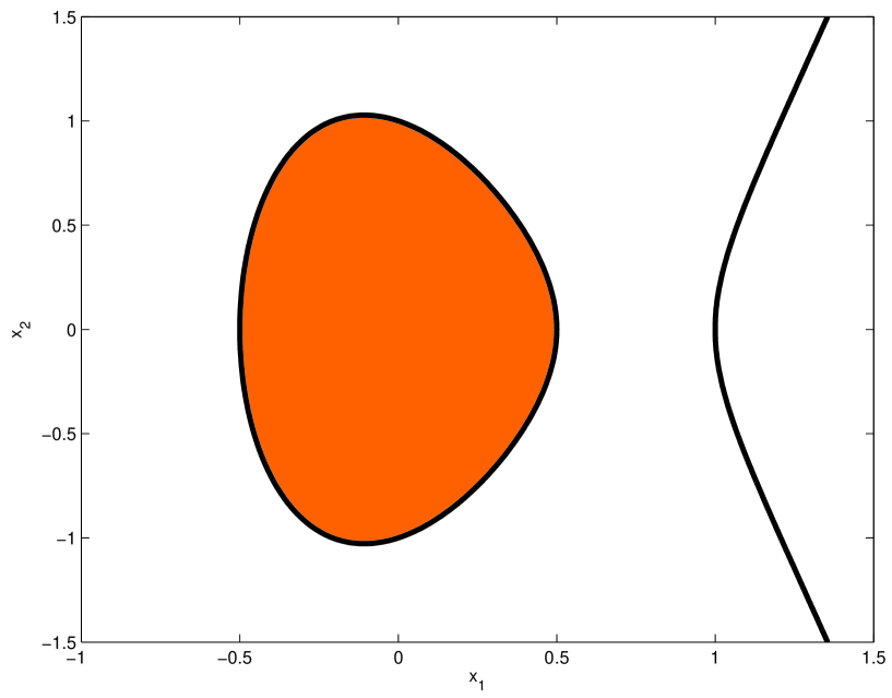
Figure 2: Cubic curve and its component around the origin (shaded).

Using the substitution (6) we obtain

$$q(t)=12(z+z^{-1})+4(z^{3}+z^{-3})-(10+3(z^{2}+z^{-2}))t-(z+z^{-1})t^{2}+t^{3}.$$

From the companion matrix

$$C=\left[\begin{array}[]{ccc}z+z^{-1}&10+3(z^{2}+z^{-2})&-12(z+z^{-1})-4(z^{3}+z^{-3})\\ 1&0&0\\ 0&1&0\end{array}\right]$$

we build (symbolically) the Hermite matrix

$$H(z)=\left[\begin{array}[]{ccc}3&\star&\star\\ z+z^{-1}&22+7(z^{2}+z^{-2})&\star\\ 22+7(z^{2}+z^{-2})&6(z+z^{-1})-2(z^{3}+z^{-3})&250+124(z^{2}+z^{-2})+15(z^{4}+z^{-4})\end{array}\right].$$

Solving (numerically) the LMI (8) with SeDuMi interfaced with YALMIP yields the spectral factorization (9) with factor (in Matlab notation)

$$U(z)=\left[\begin{array}[]{ccc}-0.9021-0.7094z^{2}&-0.5284z+0.2027z^{3}&-11.7639-9.6359z^{2}-1.5201z^{4}\\ 0.1925z&4.3449+1.6218z^{2}&0.7771z-0.5411z^{3}\\ 1.1578-0.5527z^{2}&0.3819z+0.1579z^{3}&2.4331-2.8689z^{2}-1.1844z^{4}\end{array}\right]$$

which certifies numerically that $p(x)$ is rigidly convex.

2.4 Example: quartic curve

Let us apply the algorithm to test rigid convexity of the TV quartic level set (3) with $p(x)=1-x_{1}^{4}-x_{2}^{4}$, see Figure 1.

We obtain $q(t)=-12-2(z^{4}+z^{-4})+t^{4}$ and the Hermite matrix

$$H(z)=\left[\begin{array}[]{cccc}4&\star&\star&\star\\ 0&0&\star&\star\\ 0&0&48+8(z^{4}+z^{-4})&\star\\ 0&48+8(z^{4}+z^{-4})&0&0\end{array}\right].$$

From the zero diagonal entries and the non-zero entries in the corresponding rows and columns we conclude that $H(z)$ cannot be positive semidefinite and hence that the TV quartic level set is not rigidly convex.

2.5 Numerical considerations

Since the Hermite matrix $H(z)$ has a Hankel structure, and positive definite symmetric Hankel matrices have a conditioning (ratio of extreme eigenvalues) which can be bounded below by an exponential function of the matrix size [4, 42], it may be appropriate to apply a congruence transformation on matrix $H(z)$, also called scaling.

For example, if $H(e^{i\theta_{0}})$ is positive definite for some $\theta_{0}$ (say $\theta_{0}=0$, but other choices are also possible), it admits a Schur factorization $H(e^{i\theta_{0}})=V^{T}DV$ with $V$ orthogonal and $D$ diagonal non-singular. If $D$ is reasonably well-conditioned, we can test positive semidefiniteness of the modified trigonometric polynomial matrix $H_{0}(z)=VD^{-1/2}H(z)D^{-1/2}V^{T}$ along the unit circle, which is such that $H_{0}(e^{i\theta_{0}})$ is the identity matrix. If $D$ is not well-conditioned, we can still use $H_{0}(z)=VH(z)V^{T}$ which is such that $H_{0}(e^{i\theta_{0}})$ is a diagonal matrix.

The impact of this data scaling on the numerical behavior of the semidefinite programming or algebraic Riccati equation solvers is however out of the scope of this paper.

3 LMI sets and rational algebraic plane curves

In the case that the algebraic curve $\mathcal{C}$ in (5) has genus zero, i.e. the curve is rationally parametrizable, an alternative algorithm can be devised to test rigid convexity of a connected component delimited by $\mathcal{C}$. The algorithm is based on elimination theory. It uses a particular symmetric form of a resultant called the Bézoutian. As a by-product, the algorithm also solves the determinantal representation problem in this case. As surveyed recently in [27], the key idea of using Bézoutians in the context of determinantal representations can be traced back to [28].

Starting from the implicit representation

$${\mathcal{C}}=\{x\in{\mathbb{R}}^{2}\>:\>p(x)=0\}$$ (10)

of curve $\mathcal{C}$, with $p(x)$ a bivariate polynomial of degree $m$, we apply a parametrization algorithm to obtain an explicit representation

$${\mathcal{C}}=\{x\in{\mathbb{R}}^{2}\>:\>x_{1}=q_{1}(u)/q_{0}(u),\>x_{2}=q_{2}(u)/q_{0}(u),\>u\in{\mathbb{R}}\}$$ (11)

with $q_{i}(u)$ univariate polynomials of degree $m$. Algorithms for parametrizing an implicit algebraic curve are described in [1, 38, 43]. An implementation by Mark van Hoeij is available in the algcurves package of Maple. The coefficients of $q_{i}(u)$ are generally found in an algebraic extension of small degree over the field of coefficients of $p(x)$.

With the help of resultants, we can eliminate the variable $u$ in parametrization (11) and recover an implicit equation (10), see [9, Section 3.3]. To address this implicitization problem, we make use of a particular resultant, the Bézoutian, see [15, Section 5.1.2]. Given two univariate polynomials $g,h$ of the same degree $m$ (if the degree is not the same, the smallest degree polynomial is considered as a degree $m$ polynomial with zero leading coefficients) build the following bivariate polynomial

$$\frac{g(u)h(v)-g(v)h(u)}{u-v}=\sum_{k=0}^{m-1}\sum_{l=0}^{m-1}b_{kl}u^{k}v^{l}$$

called the Bézoutian of $g$ and $h$, and the corresponding symmetric matrix $B(g,h)$ of size $m\times m$ with entries $b_{kl}$ bilinear in coefficients of $g$ and $h$. As shown e.g. in [15, Section 5.1.2], the determinant of the Bézoutian matrix is the resultant, so we can use it to derive the implicit equation (10) of a curve from the explicit equations (11).

Lemma 2

Given polynomials $q_{0},q_{1},q_{2}$ in (11), a polynomial $p$ in (10) is given by $p(x)=\det F(x)$ where

$$\begin{array}[]{rcl}F(x)&=&B(q_{1},q_{2})+x_{1}B(q_{2},q_{0})+x_{2}B(q_{1},q_{0})\\ &=&F_{0}+x_{1}F_{1}+x_{2}F_{2}\end{array}$$ (12)

is a symmetric pencil of size $m$.

Proof: Rewrite the system of equations (11) as

$$\begin{array}[]{rcccl}g_{1}(u)&=&q_{1}(u)-x_{1}q_{0}(u)&=&0\\ g_{2}(u)&=&q_{2}(u)-x_{2}q_{0}(u)&=&0\\ \end{array}$$

and use the Bézoutian resultant to eliminate indeterminate $u$ and obtain conditions for a point $(x_{1},x_{2})$ to belong to the curve. The Bézoutian matrix is $B(g_{1},g_{2})=B(q_{1}-x_{1}q_{0},q_{2}-x_{2}q_{0})=B(q_{1},q_{2})+x_{1}B(q_{2},q_{0})+x_{2}B(q_{1},q_{0})$. Linearity in $x$ follows from bilinearity of the Bézoutian and the common factor $q_{0}(u)$.$\Box$

Lemma 2 provides an implicit equation of curve (10) in symmetric linear determinantal form.

3.1 Detecting rigid convexity

Once polynomial $p(x)$ is in symmetric linear determinantal form as in Lemma 2, checking rigid convexity of the connected component containing the origin $x=0$ amounts to testing positive definiteness of $F(0)=F_{0}=B(q_{1},q_{2})$.

Lemma 3

The Bézoutian matrix $B(q_{1},q_{2})$ is positive semidefinite if and only if polynomial $q_{1}(u)$ and $q_{2}(u)$ have only real roots that interlace.

Proof: The signature (number of positive eigenvalues minus number of negative eigenvalues) of the Bézoutian of $q_{1}(u)$ and $q_{2}(u)$ is the Cauchy index of the rational function $q_{1}(u)/q_{2}(u)$, the number of jumps of the function from $-\infty$ to $+\infty$ minus the number of jumps from $+\infty$ to $-\infty$, see [2, Definition 2.53] or [2, Theorem 9.4]. It is maximum when $B(q_{1},q_{2})$ is positive definite. This occurs if and only if the roots of $q_{1}(u)$ and $q_{2}(u)$ are all real and interlace.$\Box$

Lemma 4

The connected component around the origin delimited by curve (10) is rigidly convex if and only if $B(q_{1},q_{2})\succeq 0$.

Proof: Since $F_{0}\succeq 0$, the set admits the LMI representation $\{x\in{\mathbb{R}}^{2}\>:\>F(x)\succeq 0\}$, which is equivalent to being rigidly convex. $\Box$

3.2 Finding a rigidly convex component

If the connected component around the origin is not ridigly convex, it may happen that there is another rigidly convex connected component elsewhere. To find it, it suffices to determine a point $x^{*}$ such that $F(x^{*})\succeq 0$. This is equivalent to solving a bivariate LMI problem.

We can apply primal-dual interior-point methods [33] to solve this semidefinite programming problem, since the function $f(x)=-\log p(x)=\log\det F(x)^{-1}$ is a strictly convex self-concordant barrier for the interior of the LMI set. If the LMI set is bounded, minimizing $f(x)$ yields the analytic center of the set. If the LMI set is empty, the dual semidefinite problem yields a Farkas certificate of infeasibility. However, in the bivariate case a point $x^{*}$ satisfying $F(x^{*})\succeq 0$ can be found more easily with real algebraic geometry and univariate polynomial root extraction.

A first approach consists in identifying the local minimizers of function $f(x)$. They are such that the gradient $g(x)$ of $p(x)$ vanishes, i.e. they are such that

$$g_{i}(x)=\frac{\partial p(x)}{\partial x_{i}}=\mathrm{trace}(p(x)F^{-1}(x)F_{i})=0.$$ (13)

We can characterize these minimizers by eliminating one variable, say $x_{1}$, from the system $g_{1}(x)=g_{2}(x)=0$, and solving for the other variable $x_{2}$ via polynomial root extraction. Resultants can be used for that purpose.

A second approach consists in finding points on the boundary of the LMI set, which are such that $p(x)=0$ and either $g_{1}(x)=0$ or $g_{2}(x)=0$. Here too, resultants can be applied to end up with a polynomial root extraction problem.

From the points generated by these two procedures, we keep only those satisfying $F(x)\succeq 0$, an inequality that can be certified by testing the signs of the coefficients of the characteristic polynomial of $F(x)$, as explained in the introduction.

3.3 Example: capricorn curve

Let $p(x)=x_{1}^{2}(x_{1}^{2}+x_{2}^{2})-2(x_{1}^{2}+x_{2}^{2}-x_{2})^{2}$. With the parametrization function of the algcurves package of Maple, we obtain a rational parametrization

$$\begin{array}[]{rcl}q_{0}(t)&=&45-8t+10t^{2}+t^{4}\\ q_{1}(t)&=&-7+44t-18t^{2}-4t^{3}+t^{4}\\ q_{2}(t)&=&49-28t-10t^{2}+4t^{3}+t^{4}.\end{array}$$

With the BezoutMatrix function of the LinearAlgebra package, we build the corresponding symmetric pencil

$$\small F(x)=\left[\begin{array}[]{cccc}8-4x_{1}-4x_{2}&\star&\star&\star\\ 8+20x_{1}-28x_{2}&40+60x_{1}+92x_{2}&\star&\star\\ -72+20x_{1}+52x_{2}&-8-36x_{1}-84x_{2}&776+540x_{1}+476x_{2}&\star\\ 56-4x_{1}-52x_{2}&-168+180x_{1}+180x_{2}&-952-940x_{1}+740x_{2}&1960-868x_{1}-1924x_{2}\end{array}\right]$$

whose determinant (up to a constant factor) is equal to $p(x)$. The eigenvalues of $F(0)$ are equal to $0$ (double) and $1392\pm 48\sqrt{533}$. They are all non-negative which indicates that the origin lies on the boundary of an LMI region defined by $F(x)\succeq 0$.

Values of $x_{2}$ at local optima satisfying the system of cubic equations (13) can be found with Maple as follows:

> p:=x1^2*(x1^2+x2^2)-2*(x1^2+x2^2-x2)^2:
> solve(resultant(diff(p,x1),diff(p,x2),x1));
0, 0, 0, 1, 1/2, 3+sqrt(5), 3-sqrt(5), 3+sqrt(5), 3-sqrt(5)

from which it follows that, say, the point $x_{1}=0$, $x_{2}=1/2$ is such that $F(x)\succ 0$.

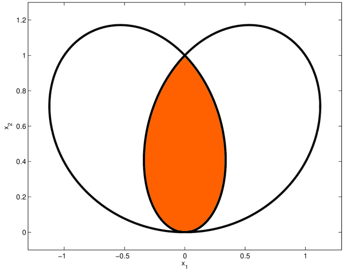
Figure 3: Capricorn curve defining an LMI region (shaded).

The corresponding LMI region together with the quartic capricorn curve are represented on Figure 3.

3.4 Example: bean curve

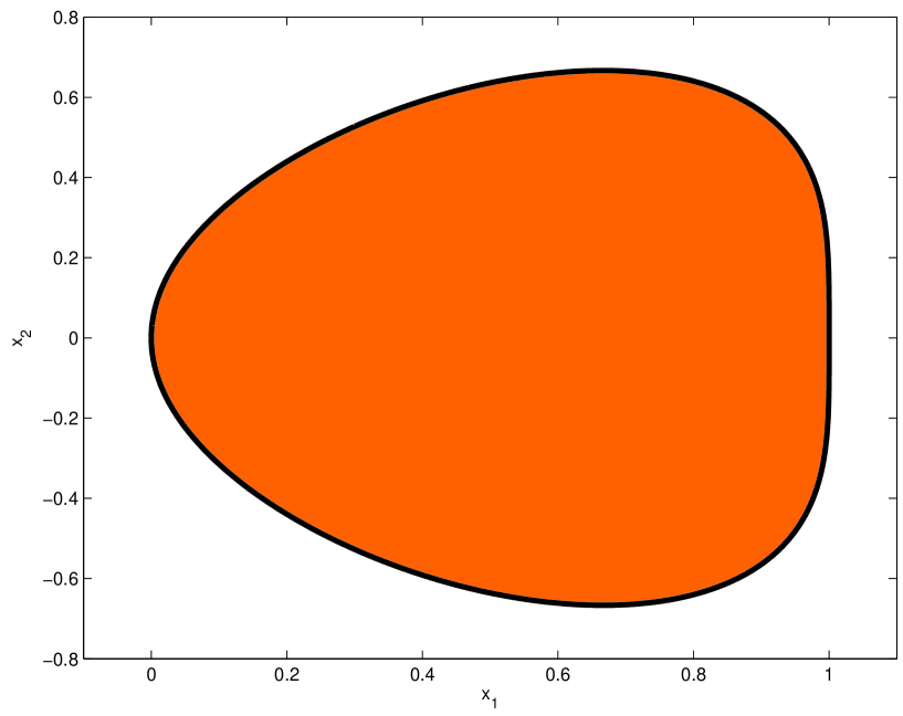
Figure 4: Bean curve defining a region which is not LMI (shaded).

Let $p(x)=x_{1}^{4}+x_{1}^{2}x_{2}^{2}+x_{2}^{4}-x_{1}^{3}+x_{1}x_{2}^{2}$. With the Bézoutians we obtain the following pencil

$$F(x)=\left[\begin{array}[]{cccc}x_{1}&\star&\star&\star\\ x_{2}&1&\star&\star\\ x_{1}&x_{2}&0&\star\\ x_{2}&1-x_{1}&0&1-x_{1}\end{array}\right].$$

We can check that $F(0)$ has eigenvalues $2$ and $0$ (triple) and this is the only point for which $F(x)\succeq 0$. It follows that the convex set delimited by the curve $p(x)=0$ is not LMI, see Figure 4.

4 Extensions

In this paragraph we outline some potential extensions of the results to algebraic plane curves of positive genus and varieties of higher dimensions.

4.1 Cubic plane curves

The case of cubic plane algebraic curves is well understood, see e.g. [44] or [40]. Singular cubics (genus zero) can be handled via Bézoutians as in Section 3. Smooth cubics (genus one), also called elliptic curves, can be handled via their Hessians.

Let $p(x_{1},x_{2})$ be a cubic polynomial that we homogeneize to $p(x_{0},x_{1},x_{2})=x_{0}^{3}p(x_{1}/x_{0},x_{2}/x_{0})$. Define its 3-by-3 symmetric Hessian matrix $H(p(x))$ with entries

$$H_{ij}=\frac{\partial^{2}p(x)}{\partial x_{i}\partial x_{j}}$$

and the corresponding Hessian $h(x)=\det H(p(x))$. The elliptic curve $p(x)=0$ has 9 inflection points, or flexes, satisfying $p(x)=h(x)=0$, and 3 of them are real. Since $p(x)$ and $h(x)$ share the same flexes and the Hessian matrix yields a symmetric linear determinantal representation for $h(x)$, we can use homotopy to find a determinantal representation for $p(x)$.

For real $t$ define the parametrized Hessian $g(x,t)=\det H(h(x)+tp(x))$ and find $t^{*}$ satisfying $g(x^{*},t^{*})=p(x^{*})$ at a real flex $x^{*}$ by solving a cubic equation. As a result, we obtain three distinct symmetric pencils not equivalent by congruence transformation. One of the may be definite hence LMI.

For example, let $p(x)=x_{1}^{3}-x_{2}^{2}-x_{1}$. Build the Hessian $h(x)=\det H(p(x))=8(x_{0}^{3}+3x_{0}x_{1}^{2}-3x_{1}x_{2}^{2})$ and the parametrized Hessian $g(x,t)=\det H(h(x)+tp(x))=24t^{3}x_{0}x_{1}^{2}-576t^{2}x^{2}_{0}x_{1}+\cdots+110592x_{1}^{3}$. Polynomial $g(x,t)$ matches $g(x)$ at flex $x^{*}_{0}=0$ for $t^{*}\in\{0,24,-24\}$ yielding the following three representations

$$\begin{array}[]{rcl}F^{1}(x)&=&\left[\begin{array}[]{ccc}1&\star&\star\\ -x_{2}&-x_{1}&\star\\ x_{1}&0&1\end{array}\right]\\ \\ F^{2}(x)&=&4^{-\frac{1}{3}}\left[\begin{array}[]{ccc}1+3x_{1}&\star&\star\\ -x_{2}&-1-x_{1}&\star\\ -1+x_{1}&-x_{2}&1-x_{1}\end{array}\right]\\ \\ F^{3}(x)&=&4^{-\frac{1}{3}}\left[\begin{array}[]{ccc}1-3x_{1}&\star&\star\\ -x_{2}&1-x_{1}&\star\\ 1+x_{1}&x_{2}&1+x_{1}\end{array}\right]\end{array}$$

such that $\det F^{i}(x)=p(x)$ for all $i=1,2,3$. Only the first one generates an LMI set $F^{1}(x)\succeq 0$.

4.2 Positive genus plane curves

The case of algebraic plane curves of positive genus and degree equal to four (quartic) or higher is mostly open. Whereas rigid convexity of higher degree polynomials can be checked with the proposed approach, there is no known implementation of an algorithm that produces symmetric linear determinantal (and hence LMI) representations in this case. For quartics, contact curves can be recovered from bitangents. In [14] complex symmetric linear determinantal representations of the quartic $1+x^{4}_{1}+x^{4}_{2}$ could be derived from the equations of the bitangents found previously by Cayley for this particular curve.

Bézoutians can be generalized to the multivariate case, as surveyed in [15]. In Lemma 2 we derived a symmetric linear determinantal representation by eliminating the variable $u$ in the system of equations

$$\begin{array}[]{rclcl}g_{1}(u)&=&q_{1}(u)-x_{1}q_{0}(u)&=&0\\ g_{2}(u)&=&q_{2}(u)-x_{2}q_{0}(u)&=&0\\ \end{array}$$

corresponding to a rational parametrization $x_{1}(u)=q_{1}(u)/q_{0}(u)$, $x_{2}(u)=q_{2}(u)/q_{0}(u)$ of the curve $p(x_{1},x_{2})=0$. In the positive genus case, such a rational parametrization is not available, but we can still define a system of equations

$$\begin{array}[]{rclcl}g_{1}(u_{1},u_{2})&=&x_{1}-u_{1}&=&0\\ g_{2}(u_{1},u_{2})&=&x_{2}-u_{2}&=&0\\ g_{3}(u_{1},u_{2})&=&p(u_{1},u_{2})&=&0\end{array}$$

describing the curve $p(x_{1},x_{2})=0$ after eliminating variables $u_{1}$ and $u_{2}$. Define the discrete differentials

$$\partial_{1}g(u,v)=\frac{g(u_{1},u_{2})-g(v_{1},v_{2})}{u_{1}-v_{1}},\quad\partial_{2}g(u,v)=\frac{g(v_{1},u_{2})-g(v_{1},v_{2})}{u_{2}-v_{2}}$$

and the quadratic form

$$\det\left[\begin{array}[]{ccc}g_{1}&\partial_{1}g_{1}&\partial_{2}g_{1}\\ g_{2}&\partial_{1}g_{2}&\partial_{2}g_{2}\\ g_{3}&\partial_{1}g_{3}&\partial_{2}g_{3}\end{array}\right]=\det\left[\begin{array}[]{ccc}x_{1}-u_{1}&-1&0\\ x_{2}-u_{2}&0&-1\\ p(u_{1},u_{2})&\partial_{1}p(u,v)&\partial_{2}p(u,v)\end{array}\right]=\sum_{\alpha,\beta}f_{\alpha,\beta}u^{\alpha}v^{\beta}$$

using bi-indices $\alpha$ and $\beta$. Then the matrix $F(x)$ of the quadratic form is a symmetric pencil satisfying $\det F(x)=p(x)q(x)$ where $q(x)$ is an extraneous factor. We hope that $q(x)$ does not depend on $x$, even though this cannot be guaranteed in general. For example, in the case of the Fermat curve $p(x)=1-x^{4}_{1}-x^{4}_{2}$ whose genus is three, using the multires package for Maple [6], we could obtain

$$F(x)=\left[\begin{array}[]{ccccccc}-1&0&0&0&0&x_{1}&x_{2}\\ 0&0&0&x_{1}&0&-1&0\\ 0&0&0&0&x_{2}&0&-1\\ 0&x_{1}&0&-1&0&0&0\\ 0&0&x_{2}&0&-1&0&0\\ x_{1}&-1&0&0&0&0&0\\ x_{2}&0&-1&0&0&0&0\end{array}\right]$$

which is such that $\det F(x)=-p(x)$, i.e. $q(x)=-1$.

4.3 Surfaces and hypersurfaces

The case $n=m=3$, i.e. cubic surfaces, is well understood, see [7] for a full constructive development. All the self-adjoint linear determinantal representations can be obtained from the tritangent planes. The number of non-equivalent representations depends on the number and class of real lines among the 27 complex lines of the surface. See [39] for a nice survey on cubic surfaces.

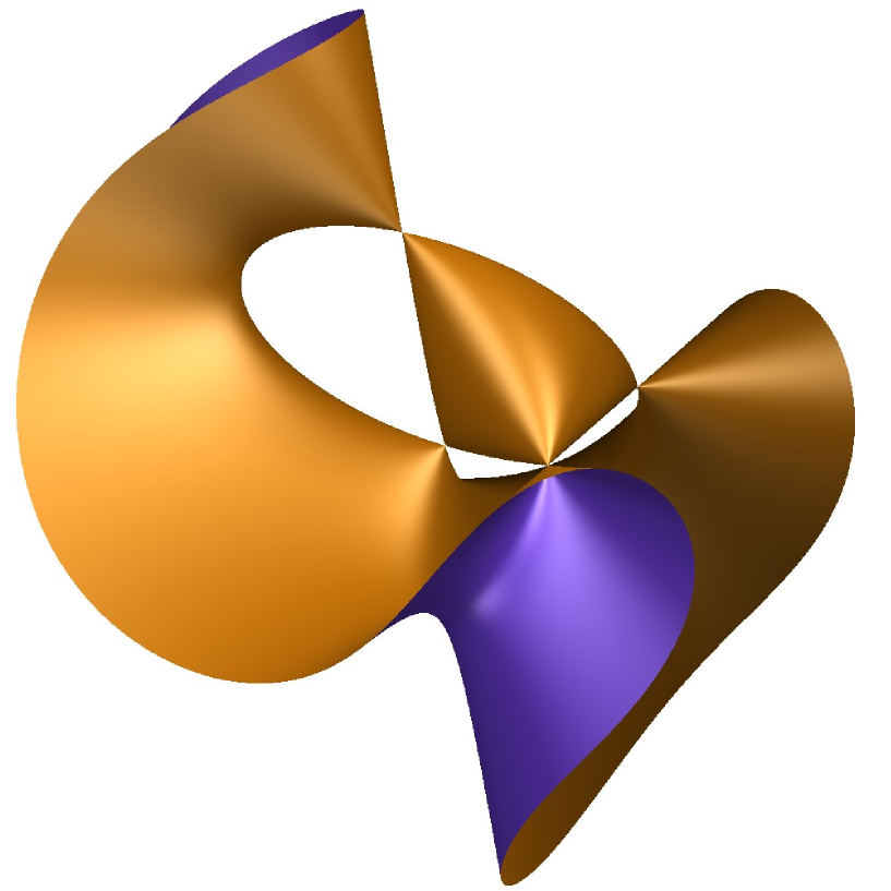
Figure 5: The Cayley cubic surface with its convex connected component.

A well-known example is the Cayley cubic

$$\frac{1}{u_{0}}+\frac{1}{u_{1}}+\frac{1}{u_{2}}+\frac{1}{u_{3}}=0$$

whose algebraic equation is

$$u_{0}u_{1}u_{2}+u_{0}u_{1}u_{3}+u_{0}u_{2}u_{3}+u_{1}u_{2}u_{3}=0.$$

Under involutary linear mapping

$$\left[\begin{array}[]{c}x_{0}\\ x_{1}\\ x_{2}\\ x_{3}\end{array}\right]=\frac{1}{2}\left[\begin{array}[]{cccc}1&1&1&1\\ 1&1&-1&-1\\ 1&-1&1&-1\\ 1&-1&-1&1\end{array}\right]\left[\begin{array}[]{c}u_{0}\\ u_{1}\\ u_{2}\\ u_{3}\end{array}\right]$$

the dehomogenized ($x_{0}=1$) algebraic equation becomes

$$p(x)=1-x_{1}^{2}-x_{2}^{2}-x_{3}^{2}-2x_{1}x_{2}x_{3}=\det\left[\begin{array}[]{ccc}1&x_{1}&x_{2}\\ x_{1}&1&x_{3}\\ x_{2}&x_{3}&1\end{array}\right]=\det F(x)$$

which is the determinant of the 3x3 moment matrix of the MAXCUT LMI relaxation. The surface $p(x)=0$ is represented on Figure 5, using the surf visualization package. In particular, we can easily identify the convex connected component containing the origin, described by the LMI $F(x)\succeq 0$. The component has four vertices, or singularities, for which the rank of $F(x)$ drops down to one.

In general, only curves and cubic surfaces admit generically a determinantal representation. When $n>3$ or $m>3$ and no lifting is allowed, the hypersurface $p(x)=0$ must be highly singular to have a determinantal representation [3], and hence, a fortiori, an LMI representation. This leaves however open the existence of alternative algorithms consisting in constructing symmetric linear determinantal representations of modified polynomials $p(x)q(x)$, with $q(x)$ globally nonnegative, say $q(x)=(\sum_{i}x^{2k}_{i})$ or $(\sum_{i}x_{i})^{2k}$ for $k\geq 1$ large enough.

Finally, let us conclude by remarking that, as a by-product of the proof leading to Lemma 1, checking numerically rigid convexity of a scalar polynomial when $n>2$ amounts to checking positivity of a multivariate Hermite matrix. See e.g. [13] for recent developments on the use of semidefinite programming for multivariate trigonometric polynomial matrix positivity.

References

- [1] S. S. Abhyankar, C. L. Bajaj. Automatic parameterization of rational curves and surfaces III: Algebraic plane curves. Computer Aided Geom. Design 5:309–321, 1988.
- [2] S. Basu, R. Pollack, M.-F. Roy. Algorithms in real algebraic geometry. Springer, 2003.
- [3] A. Beauville. Determinantal hypersurfaces. Michigan Math. J. 8:39–64, 2000.
- [4] B. Beckermann. The condition number of real Vandermonde, Krylov and positive definite Hankel matrices. Numer. Mathematik, 85:553-577, 2000.
- [5] A. Ben-Tal, A. Nemirovskii. Lectures on modern convex optimization. SIAM, 2001.
- [6] L. Busé, B. Mourrain, I.Z. Emiris, O. Ruatta, J. Canny, P. Pedersen, I. Tonelli. Using the Maple multires package. INRIA Sophia-Antipolis, France, 2003.
- [7] A. Buckley, T. Košir. Determinantal representations of smooth cubic surfaces. Geometriae Dedicata, 125:115–140, 2007.
- [8] F. M. Callier. On polynomial matrix spectral factorization by symmetric extraction. IEEE Trans. Autom. Control, 30(5):453–464, 1985.
- [9] D. Cox, J. Little, D. O’Shea. Ideals, varietes, and algorithms. Springer, 1992.
- [10] B. Deconinck, M. S. Patterson. Computing the Abel map. Preprint, Dept. Applied Math., Univ. Washington, Seattle, 2007.
- [11] B. Deconinck, M. van Hoeij. Computing Riemann matrices of algebraic curves. Phys. D 152/153:123–152, 2001.
- [12] A. C. Dixon. Note on the reduction of a ternary quantic to a symmetrical determinant. Proc. Cambridge Phil. Soc. 11:350–351, 1902.
- [13] B. Dumitrescu. Positive trigonometric polynomials and signal processing applications. Springer, 2007.
- [14] W. L. Edge. Determinantal representations of . Proc. Cambridge Phil. Soc. 34:6–21, 1938.
- [15] M. Elkadi, B. Mourrain. Introduction à la résolution des systèmes polynomiaux. Springer, 2007.
- [16] H. M. Farkas, I. Kra. Riemann surfaces. 2nd ed. Springer, 1992.
- [17] Y. Genin, Y. Hachez, Y. Nesterov, R. Ştefan, P. Van Dooren, S. Xu. Positivity and linear matrix inequalities. European J. Control, 8(3):275–298, 2002.
- [18] Y. Genin, Y. Hachez, Y. Nesterov, P. Van Dooren. Optimization problems over positive pseudo-polynomial matrices. SIAM J. Matrix Anal. Appl., 25(1):57–79, 2003.
- [19] I. Gohberg, P. Lancaster, I. Rodman. Matrix polynomials, Academic Press, 1982.
- [20] P. A. Griffiths. Introduction to algebraic curves. AMS, 1989.
- [21] S. Hecker, A. Varga, J. F. Magni. Enhanced LFR toolbox for Matlab. Proc. IEEE Symp. Computer Aided Control System Design, Taiwan, 2004.
- [22] J. W. Helton, S. A. McCullough, V. Vinnikov. Noncommutative convexity arises from linear matrix inequalities. J. Functional Analysis 240(1):105–191, 2006.
- [23] J. W. Helton, V. Vinnikov. Linear matrix inequality representation of sets. Comm. Pure Applied Math. 60(5):654–674, 2007.
- [24] J. W. Helton, J. Nie. Sufficient and necessary conditions for semidefinite representability of convex hulls and sets. arXiv:0709.4017, September 2007.
- [25] D. Henrion, M. Šebek. An efficient numerical method for the discrete-time symmetric matrix polynomial equation. IEE Proc. Control Theory Appl. 145(5):443–448, 1998.
- [26] J. Ježek, V. Kučera. Efficient algorithm for matrix spectral factorization. Automatica, 21(6):663-669, 1985.
- [27] S. Kaplan, A. Shapiro, M. Teicher. Several applications of Bézout matrices. arXiv:math.AG/0601047, January 2006.
- [28] N. Kravistky. On the discriminant function of two commuting non-selfadjoint operators. Integral Equ. Operator Theory, 3(1):97–124, 1980.
- [29] H. Kwakernaak, M. Šebek. Polynomial J-Spectral Factorization. IEEE Trans. Autom. Control, 39(2):315–328, 1994.
- [30] J. B. Lasserre. Convex sets with lifted semidefinite representation. LAAS-CNRS Research Report No. 07034, January 2007.
- [31] A. S. Lewis, P. A. Parrilo, M. V. Ramana. The Lax conjecture is true. Proc. Amer. Math. Soc. 133(9):2495–2499, 2005.
- [32] T. Meyer-Brandis. Berührungssysteme und symmetrische Darstellungen ebener Kurven. Diplomarbeit, Univ. Mainz, 1998.
- [33] Y. Nesterov, A. Nemirovskii. Interior point polynomial algorithms in convex programming, SIAM, 1994.
- [34] J. Piontkowski. Linear symmetric determinantal hypersurfaces. Michigan Math. J. 54:117-146, 2006.
- [35] PolyX, Ltd. The Polynomial Toolbox for Matlab. 1998.
- [36] J. Renegar. Hyperbolic programs and their derivative relaxations. Foundations Comput. Math. 6(1):59–79, 2006.
- [37] T. G. Room. The geometry of determinantal loci. Cambridge Univ. Press, 1938.
- [38] J. R. Sendra, F. Winkler. Symbolic parametrization of curves. J. Symbolic Comput. 12(6):607–631, 1991.
- [39] I. Szilágyi. Symbolic-numeric techniques for cubic surfaces. PhD Thesis, RISC, Univ. Linz, Austria, 2005.
- [40] O. Taussky. Nonsingular cubic curves as determinantal loci. J. Math. Phys. Sci. 21(6):665–678, 1987.
- [41] H. L. Trentelman and P. Rapisarda. New algorithms for polynomial J-spectral factorization. Math. Control Signals Systems, 12:24–61, 1999.
- [42] E. E. Tyrtyshnikov. How bad are Hankel matrices ? Numer. Math. 67:261–269, 1994.
- [43] M. van Hoeij. Rational parametrization of curves using canonical divisors. J. Symbolic Comput. 23:209–227, 1997.
- [44] V. Vinnikov. Self-adjoint determinantal representations of real irreducible cubics. In: Operator Theory - Advances and Applications, Vol. 19, Birkhäuser, 1986.
- [45] V. Vinnikov. Self-adjoint determinantal representations of real plane curves. Math. Annalen, 296:453–479, 1993.
- [46] J. C. Willems. Least squares stationary optimal control and the algebraic Riccati equation. IEEE Trans. Autom. Control, 16(6):621–634, 1971.
- [47] V. A. Yakubovich. Factorization of symmetric matrix polynomials. Dokl. Acad. Nauk. SSSR, 194(3):1261–1264, 1970.
- [48] J. C. Zúñiga, D. Henrion. A Toeplitz algorithm for polynomial J-spectral factorization. Automatica, 42(7):1085–1093, 2006.