Spontaneous symmetry breakdown in fuzzy spheres

Abstract

We study and analyse the questions regarding breakdown of global symmetry on noncommutative sphere. We demonstrate this by considering a complex scalar field on a fuzzy sphere and isolating Goldstone modes. We discuss the role of nonlocal interactions present in these through geometrical considerations.

I Introduction

Recently there has been interest in the non-perturbative numerical studies of quantum fields on fuzzy spaces. This was motivated by the fact that implementation of noncommutative geometry appears through novel features in such models. For example, the IR/UV mixing, even though absent in the finite matrix setting appears through an anomaly which generates it in the continuum limit. This suggests the possibility that fuzzy spaces may serve as novel regulators of field theories and bring out new features which were absent in the conventional lattice regularisations. This program falls well within the front line of research activity of study of noncommutative geometry hoppe ; madore ; pinzul ; sbal ; xavier ; denjoe ; steinaker ; bietenholz ; panero ; das .

Earlier studies on simulations have focused on scalar fields on fuzzy spheres ($\displaystyle S_{F}^{2}$) and led to the demonstration of new phases characterised as nonuniform ordered phase denjoe ; bietenholz ; panero ; das . In the continuum infinite volume limit this nonuniform phase appears as stripe phase in the Groenewold-Moyal space gubser ; ambjorn . These nonuniform phases are related to the existence of meta stable states and we have demonstrated this in our earlier analysis using what is known as pseudo heat bath method das . We could also show the existence of meta stable states as well as their connections to many phases.

Those new “stripe” phases were conjectured by Gubser and Sondhi gubser , where they pointed out that this translation non-invariant phase would exist only in dimensions $\displaystyle d\geq 3$. However the numerical simulation of Ambjorn and Catterall show the existence of such a phase even in $\displaystyle d=2$ ambjorn . This seems to be contradicting Coleman-Mermin-Wagner(CMW) theorem that continuous symmetries cannot be broken spontaneously in $\displaystyle d=2$ mermin . But CMW theorem can be expected to be valid only in local field theories paolo . On the other hand NC field theories are inherently nonlocal and can be expected to show new features. However Gubser and Sondhi while analysing NC field theories point out that the infrared problems are worse in these theories and hence CMW theorem cannot be violated. But numerical simulations show the results to be other way. In this connection it is important to see whether long range order or symmetry breaking can be seen for global symmetries other than space time symmetries. This assumes importance, since Gubser and Sondhi explicitly use $\displaystyle O(N)$ and $\displaystyle O(2)$ symmetries in showing their results.

We analyse in this paper this important question, namely what happens to CMW theorem and long range order in the fuzzy spaces paolo . We consider a complex scalar field theory with a global $\displaystyle U(1)$ and study the full implications of the noncommutative nature of the underlying geometry. As pointed out earlier spontaneous symmetry breakdown (SSB) and long range order are obstructed in $\displaystyle 2D$ theories by the infrared divergences associated with Goldstone modes. While nonlocal field theories can escape these conditions, it is not obvious whether they do so in these circumstances.

This paper is organised as follows: In Sec.2 we describe the model, notations and address the questions. In Sec.3 we look at the aspects of simulations and demonstrate the spontaneous breaking of $\displaystyle U(1)$ symmetry thereby evading CMW theorem. In Sec.4, we analyse questions of Goldstone modes, the role of non-locality and subtle issues in isolating effects of continuum limit as well as infinite volume limit. In the last Sec.5, we present our results and conclusions, taking into account already existing theoretical studies.

II SSB on $\displaystyle 2D$ NC space and CMW theorem

The standard action used for studying the $\displaystyle U(1)$ in two dimensional ($\displaystyle 2D$) Moyal spaces is given as gubser ,

$$S=\int d^{2}x\left[|\partial\Phi|^{2}+r|\Phi|^{2}+\lambda_{1}\Phi{\bf\star}\Phi{\bf\star}\Phi^{*}{\bf\star}\Phi^{*}+\lambda_{2}\Phi{\bf\star}\Phi^{*}{\bf\star}\Phi{\bf\star}\Phi^{*}\right]$$ (1)

Finite temperature behaviour of the $\displaystyle\Phi$ field with fluctuations is studied by varying the mass parameter $\displaystyle r$. One would expect the average of $\displaystyle\Phi$ to take the form,

$$\langle|\Phi|\rangle=\sqrt{-{\frac{r}{2(\lambda_{1}+\lambda_{2})}}}\,$$ (2)

in the mean-field theory. In commutative two dimensional space the $\displaystyle U(1)$ Goldstone mode destroys the above condensate. So, there will not be SSB of the $\displaystyle U(1)$ symmetry in these spaces. As discussed above, the status of $\displaystyle U(1)$ SSB is not clear in $\displaystyle 2D$ NC spaces. Very little has been done from the non-perturbative side to study this issue.

We will present in this note that the spontaneous breaking of internal symmetries can be expected in Moyal space times when space-time symmetries are broken. Conventionally the obstruction to SSB in $\displaystyle 2D$ will come through the infrared divergence from the resulting massless Goldstone boson. Gubser and Sondhi argued that the infrared behaviour is worse in $\displaystyle 2D$ NC space and hence will continue to obey CMW theorem. But the simulations point out that this to be not the case. We will argue how this can be understood with specific requirements in these theories.

To obtain SSB of $\displaystyle U(1)$ we should have the complex field $\displaystyle\Phi$ in the ground state such that

$$\int\Phi\,d^{2}x=0\quad\rm{and}\quad\Phi\neq 0\,.$$ (3)

This will translate to $\displaystyle Tr\Phi=0$ in Moyal space. This implies that when $\displaystyle\Phi$ is expanded in Fourier modes $\displaystyle\tilde{\Phi}(k)$, the zero mode should be absent. That is,

$$\tilde{\Phi}(k=0)=0\,.$$

Correspondingly, on the sphere $\displaystyle\Phi$ should not have a singlet component in the angular momentum basis. This naturally gives a cutoff $\displaystyle k_{c}$ fixed by the parameters of the effective action including quantum fluctuations. This cut-off in the integral avoids infrared singularities. The important factor responsible for this is the existence of states which are not translationally invariant, such as the stripe phase (or nonuniform phase). Hence $\displaystyle U(1)$ can be broken spontaneously only along with translation symmetry violating nonuniform phase. We will see how these features appear in our simulation studies.

III Simulations on Fuzzy $\displaystyle S^{2}$

In this work we study this problem non-perturbatively on a fuzzy sphere. The fuzzy spheres are described by the coordinates $\displaystyle X_{i}$ obeying the algebra

$$\left[X_{i},X_{j}\right]=\frac{i\alpha\epsilon_{ij}{{}^{k}}X_{k}}{{\sqrt{j(j+1)}}},~{}~{}~{}\sum_{i}X_{i}^{2}=R^{2}.$$ (4)

Here $\displaystyle R$ is the radius of the fuzzy sphere. $\displaystyle\alpha/\sqrt{j(j+1)}$ measures the non commutativity in the fuzzy sphere. Here $\displaystyle\alpha$ is a function of $\displaystyle R$. On the fuzzy sphere the above action (Eq.1) reduces to,

$$S(\Phi)=\frac{4\pi}{N}\,{\rm Tr}\left[\sum_{i}|\left[L_{i},\Phi\right]|^{2}+R^{2}\left(r|\Phi|^{2}+\lambda_{1}\Phi\Phi\Phi^{{\dagger}}\Phi^{{\dagger}}+\lambda_{2}\Phi\Phi^{{\dagger}}\Phi\Phi^{{\dagger}}\right)\right].$$ (5)

Here the real and imaginary parts of $\displaystyle\Phi\in{\rm Mat}_{N}$ are $\displaystyle N\times N$ hermitian matrices. The quartic terms represent the self interaction of the $\displaystyle\Phi$ field. These terms are crucial for the presence of noncommutativity and nonlocality in this problem. In the following we describe our strategy of studying the SSB of $\displaystyle U(1)$ and the numerical simulations.

The simulation of the above model for the SSB study of $\displaystyle U(1)$ in fuzzy $\displaystyle S^{2}$ involves generating statistically relevant matrix configurations for a particular choice of parameters. The configurations are generated using “pseudo-heatbath” method, for details see das . The auto-correlation for larger $\displaystyle N$ simulations turn out to be large. To reduce the autocorrelation problem we use over-relaxation algorithm. However the number of over-relaxation steps required grows with $\displaystyle N$ rapidly. This makes it difficult to get any reasonable statistics for large $\displaystyle N$.

The CMW theorem and SSB for finite systems is subtle. For a finite system there will be tunnelling between all possible vacua, though the tunnelling rate is exponentially suppressed as the size of the system increases. Because of the tunnelling, the state of the system respects the symmetry. However this state of the system is unlike the symmetry restored state at high temperatures. In this situation ensemble average of the magnitude of the “magnetisation” is usually taken to be the condensate (order parameter). Using this prescription we look for SSB of continuous symmetry for finite systems in $\displaystyle 2D$. In order to numerically prove the CMW theorem one has to show that the condensate vanishes in the infinite volume limit. The numerical study of finite size effects in commutative $\displaystyle 2D$ show that the condensate vanishes logarithmically. One should expect that there will also be finite size effects for noncommutative spaces. So the finite $\displaystyle R,N$ effects must be separated out to settle the issue of $\displaystyle U(1)$ SSB on fuzzy sphere. There are various limits possible consistent with $\displaystyle(R,N)\to\infty$. We do not consider the limit $\displaystyle(R,N)\to\infty$ in which the resultant space becomes commutative and there should be no SSB of $\displaystyle U(1)$. When the ratio $\displaystyle R^{2}/N$ remains finite for $\displaystyle(R,N)\to\infty$ we have a thermodynamic limit which still maintains the non-commutative character.

The numerical simulations always consider a finite $\displaystyle N$. As discussed above a non-zero $\displaystyle\langle\Phi\rangle$ will not validate or invalidate the CMW theorem. We need to study the behaviour of $\displaystyle\langle\Phi\rangle$ for various $\displaystyle N$ to see SSB of $\displaystyle U(1)$ or otherwise. While we vary $\displaystyle N$ the ratio $\displaystyle R^{2}/N$ is kept fixed. To simplify the numerical work we choose $\displaystyle\lambda_{1}=\lambda_{2}=\lambda/2$ from the parameter space. The simulations were then done for a fixed $\displaystyle\lambda,r$. The observables we measure are action $\displaystyle S$, $\displaystyle\Phi$ and fluctuations of various elements of $\displaystyle\Phi$. Each element $\displaystyle\Phi_{ij}$ now is a complex number, so,

$$\Phi_{ij}=\eta_{ij}e^{i\theta_{ij}}.$$ (6)

Note that because of the $\displaystyle U(1)$ symmetry $\displaystyle\Phi_{ij}$ will have a circular distribution in the complex plane, with $\displaystyle\langle\eta_{ij}\rangle$ being the average radius of the distribution. A non-vanishing $\displaystyle\langle\eta_{ij}\rangle$ in the $\displaystyle N\to\infty$ limit for at least one element of $\displaystyle\Phi$ will clearly signal SSB of $\displaystyle U(1)$. In the following we discuss the simulation parameters, results and discussions.

IV Results and discussions

The parameter values we choose for our simulations are $\displaystyle\lambda=1.0$, $\displaystyle r=-8$. We have also repeated our simulations for $\displaystyle r=-16$. For these choices of parameters various values of $\displaystyle N$ starting from $\displaystyle N=16$ onwards are considered. The run time to get reasonable statistics grows rapidly with $\displaystyle N$. At present the largest value of $\displaystyle N$ we have simulated is $\displaystyle N=100$. We also have a few set of data with less statistics for $\displaystyle N>100$.

The simulation results showed that the off-diagonal elements of $\displaystyle\Phi$ are always fluctuating around zero. The change in the behaviour of these elements with $\displaystyle N$ is not so prominent. So, in this paper we show only the behaviour of diagonal elements of $\displaystyle\Phi$. In Fig.1, we show the distributions of $\displaystyle\Phi_{11},\Phi_{22}$ and $\displaystyle\Phi_{mm}$, where $\displaystyle mm$ correspond to the middle diagonal element or one of the middle diagonals if $\displaystyle N$ is even.

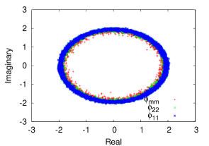
(a)  Distribution of $\displaystyle\Phi_{11},\Phi_{22}$ and $\displaystyle\Phi_{mm}$ for $\displaystyle N=19$ and $\displaystyle\rho_{0}\sim 1$.

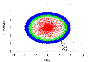
(b)  Distribution of $\displaystyle\Phi_{11},\Phi_{22}$ and $\displaystyle\Phi_{mm}$ for $\displaystyle N=64$ and $\displaystyle\rho_{0}\sim 1$.

Figure 1:

From the figure we can clearly see that the distribution has a $\displaystyle U(1)$ symmetry. The distributions of pair of elements such as $\displaystyle\Phi_{ii}$ and $\displaystyle\Phi_{N-i+1,N-i+1}$ are found to be the same as expected. In order to show finite size effects we consider $\displaystyle N=19$ and $\displaystyle N=64$ in the above figure. We see that for all $\displaystyle N$, the radii of the distributions decrease as we move towards the middle elements. The difference here is that for $\displaystyle N=19$ the radii are close to each other, but for $\displaystyle N=64$ they are different by large amount. Indeed for $\displaystyle N=64$ the middle diagonal distribution has a peak around zero in the complex plane. The difference in the property of $\displaystyle\Phi$ between $\displaystyle N=19$ and $\displaystyle N=64$ is purely finite volume effect. Also due to finite volume effects even the radius of distribution of $\displaystyle\Phi_{11}(\Phi_{NN})$ has increased from $\displaystyle N=64$ to $\displaystyle N=19$.

One of the main difference between commutative and non-commutative $\displaystyle 2D$ space is the presence of degenerate/meta-stable states in the latter. In the numerical simulations one always chooses an initial configuration. For commutative $\displaystyle 2D$, whatever may be the initial configuration, there is always a unique thermalized state. The situation is completely different in the case of fuzzy sphere. Depending on the initial configuration we get different thermalized states.

The detailed analysis of $\displaystyle\Phi$ reveals that the phase of all diagonal elements is perfectly correlated for smaller $\displaystyle N$. For example in Fig.2 we plot the phase of $\displaystyle\Phi_{11}$ vs phase of $\displaystyle\Phi_{NN}$ for $\displaystyle N=19$.

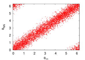
(a)  Distribution of $\displaystyle\theta_{11}$ vs $\displaystyle\theta_{NN}$ for $\displaystyle N=19$ and $\displaystyle\rho_{0}\sim 1$.

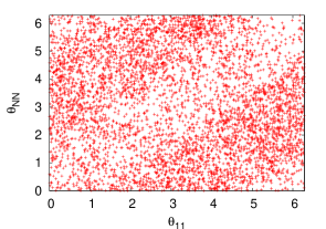
(b)  Distribution of $\displaystyle\theta_{11}$ vs $\displaystyle\theta_{NN}$ for $\displaystyle N=64$ and $\displaystyle\rho_{0}\sim 1$.

Figure 2:

We find that each configuration for $\displaystyle N=19$ the phases of all diagonal elements are fluctuating around same average value. Since the different radii for the distributions are not much different the form of $\displaystyle\Phi$, for $\displaystyle N=19$ is close to the form $\displaystyle\Phi\sim{\bf I}e^{i\theta}$. In Fig.2b we plot the phase of $\displaystyle\Phi_{11}$ vs phase of $\displaystyle\Phi_{NN}$ for $\displaystyle N=64$. Here, the correlation between $\displaystyle\theta_{11}$ and $\displaystyle\theta_{NN}$ is not as strong. These results were obtained with a initial configuration $\displaystyle\Phi_{0}=\rho_{0}{\bf 1}$, with $\displaystyle\rho_{0}\sim 1$. With the initial condition, $\displaystyle\rho_{0}\sim 0$, we get same results for $\displaystyle N=19$ as before, but for $\displaystyle N=64$ the results are dramatically different. In Fig.3 we show the distribution of $\displaystyle\Phi$ and $\displaystyle\theta_{11}~{}\rm{vs}~{}\theta_{NN}$ correlation for $\displaystyle N=64$. It can be seen from Fig.3 the correlation between $\displaystyle\theta_{11}$ and $\displaystyle\theta_{NN}$ is stronger in this case.

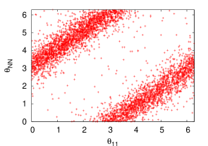
Figure 3: Distribution of $\displaystyle\theta_{11}$ vs $\displaystyle\theta_{NN}$ for $\displaystyle N=64$ and $\displaystyle\rho_{0}\sim 0$.

The difference in results for $\displaystyle N=64$ shown in Fig.2b and Fig.3 are coming from two (meta)stable states available for the system. Such (meta)stable states are absent for the same theory in commutative $\displaystyle 2D$ space. For all different initial configurations for $\displaystyle N>25$, $\displaystyle\theta_{11}$ and $\displaystyle\theta_{NN}$ were never in phase like Fig.2a. As a result $\displaystyle Tr(\Phi)$ decreases for larger $\displaystyle N$. For larger $\displaystyle N$ average of $\displaystyle Tr(\Phi)$ is found to be zero. This is expected as only these states with $\displaystyle Tr(\Phi)=0$ can survive the thermodynamic limit.

From $\displaystyle N=19$ to $\displaystyle N=64$ there is transition in the form of $\displaystyle\Phi$. Also the average of $\displaystyle\eta_{11}$ is smaller for $\displaystyle N=64$. This result clearly shows that uniform ordered phase is not a stable state in the limit $\displaystyle N\to\infty$. The transition in the form of $\displaystyle\Phi$, when $\displaystyle N$ is increased takes place around $\displaystyle N=25$ for the choice of $\displaystyle\lambda,r$ in our simulations. This can be seen in Fig.4a.

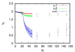
(a)  $\displaystyle N$ dependence of $\displaystyle\eta_{11},\eta_{22}$ and $\displaystyle\eta_{mm}$.

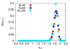
(b)  Histogram of $\displaystyle\eta_{11}$ for $\displaystyle N=40,64$ and $\displaystyle N=100$.

Figure 4:

The above results show that $\displaystyle\langle\eta_{11}\rangle$ seems to saturate for $\displaystyle N\geq 40$. In Fig.4b, we show the histogram distribution of $\displaystyle\eta_{11}$ for $\displaystyle N=40,64$ and $\displaystyle 100$. The peak of the distribution hardly changes with $\displaystyle N$. On the other hand, the width for $\displaystyle N=100$ is clearly smaller. In other words, the fluctuations of $\displaystyle\eta_{11}$ is sharply peaked. This suggests that the results for larger $\displaystyle N$ will not deviate from what we have already seen. The results shown in Fig.4a have been obtained with $\displaystyle\rho_{0}\sim 1$ for the initial configuration. We find that the results for $\displaystyle\eta_{11}$ or $\displaystyle\eta_{NN}$ hardly change with different initial configurations. Even if there is a small change, their values do not show any $\displaystyle N$ dependence for larger $\displaystyle N$. We caution, here that the statistics for $\displaystyle N>100$ are very small and the autocorrelation is substantial.

The saturation of $\displaystyle\langle\eta_{11}\rangle$ beyond $\displaystyle N=40$ up to the largest simulated $\displaystyle N$ suggests that $\displaystyle\Phi$ does not vanish in the non-commutative thermodynamic limit. The form of $\displaystyle\Phi$ we have obtained from the simulations also show that the ground state is not a uniform ordered phase, but rather a non-uniform ordered phase. This shows that all the generators, $\displaystyle L_{x},L_{y}$ and $\displaystyle L_{z}$ are spontaneously broken in the ground state. This implies that there will be three Goldstone modes.

V Conclusion

Having presented various simulations on fuzzy sphere with the intention to understand the issue of CMW theorem we will now summarise the conclusions. While considering QFT’s in Moyal space time Gubser and Sondhi gubser concluded the possibility of translation symmetry violating stripe phase in dimensions $\displaystyle d\geq 3$. Ambjorn and Catterall ambjorn have demonstrated this phase in $\displaystyle d=2$ through Monte Carlo simulations. This was followed by studies on $\displaystyle S_{F}^{2}$ and $\displaystyle S_{F}^{2}\times R$ panero ; bholz ; medina . Gubser and Sondhi also conjectured that internal symmetries like $\displaystyle O(N)$ cannot be broken, as expected from CMW theorem. But CMW theorem explicitly uses locality of interactions and NC field theories are inherently nonlocal. We have argued that the Fourier transform of the complex field should be vanishing at zero momentum, as the important criterion for global symmetry breaking phases. This translates to vanishing of the singlet component of the field in the angular momentum basis in fuzzy spheres. In our simulations we find evidence for the breaking of global symmetries in $\displaystyle 2D$ NC field theories. The existence of nonuniform stable states contribute at higher temperature, thereby breaking the translation and internal symmetries. Translation symmetry breaking stripe phase is required for obtaining the internal symmetry violation and long range order and these two occur together.

VI Acknowledgment

We thank A. P. Balachandran, W. Bietenholz and M. Panero for useful discussions and comments on the draft of this paper. We also thank G. Menon and P. Ray for clarifying issues related to the CMW theorem. We also thank A. Bigarini for sending copy of his thesis where SSB and CMW theorem in Moyal space are discussed. All the calculations have been carried out using the computer facilities at IMSc, Chennai.

References

- (1) J. Hoppe, Ph.D. Thesis, MIT (Cambridge MA, 1982).
- (2) J. Madore, Class. and Quant. Grav. 9, 69 (1992).
-
(3)
A.P. Balachandran, T.R. Govindarajan and B. Ydri,
Mod. Phys. Lett. A15, 1279 (2000) [hep-th/9911087];
A.P. Balachandran, A. Pinzul and B.A. Qureshi, JHEP 0512, 002 (2005) [hep-th/0506037]. - (4) T. Azuma, S. Bal, K. Nagao and J. Nishimura, JHEP 0405, 005 (2004) [hep-th/0401038].
- (5) A.P. Balachandran, S. Kurkcuoglu and S. Vaidya, arXiv: hep-th/0511114.
- (6) X. Martin, JHEP 0404, 077 (2004) [hep-th/0402230].
-
(7)
J. Medina, W. Bietenholz, F. Hofheinz and
D. O’Connor, PoS LAT2005, 263 (2005) [hep-lat/0509162];
F. G. Flores, D. O’Connor and X. Martin, PoS LAT2005, 262 (2006) [hep-lat/0601012];
D. O’Connor and B. Ydri, JHEP 0611, 016 (2006) [hep-lat/0606013];
J. Medina, arXiv: 0801.1284 [hep-th]. -
(8)
H. Steinacker, JHEP 0503, 075 (2005) [hep-th/0501174];
D. O’Connor and C. Saemann, JHEP 0708, 066 (2007) [0706.2493 [hep-th]]. -
(9)
W. Bietenholz, F. Hofheinz and J. Nishimura,
Acta. Phys. Polon. B34, 4711 (2003) [hep-th/0309216];
Nucl. Phys. Proc. Suppl. 129, 865 (2004) [hep-th/0309182]. -
(10)
M. Panero, SIGMA 2, 081 (2006) [hep-th/0609205];
JHEP 0705, 082 (2007) [hep-th/0608202]. - (11) C.R. Das, S. Digal and T.R. Govindarajan, arXiv: 0706.0695 [hep-th].
- (12) S.S. Gubser and S.L. Sondhi, Nucl. Phys. B605, 395 (2001) [hep-th/0006119].
- (13) J. Ambjorn and S. Catterall, Phys. Lett. B549, 253 (2002) [hep-lat/0209106].
-
(14)
N.D. Mermin and H. Wagner, Phys. Rev. Lett 17,
1133 (1966);
P.C. Hohenberg, Phys. Rev. 158, 383 (1967);
S.R. Coleman, Commun. Math. Phys. 31, 259 (1973). - (15) P. Castorina and D. Zappala, arXiv: 0711.2659 [hep-th].
- (16) W. Bietenholz, F. Hofheinz and J. Nishimura, JHEP 0406, 042 (2004) [hep-th/0404020].
- (17) J. Medina, W. Bietenholz and D. O’Connor, arXiv:0712.3366 [hep-th].