ENERGY OF INTERACTION BETWEEN SOLID SURFACES AND LIQUIDS

Henri GOUIN

L. M. M. T.   Box 322,  University of Aix-Marseille

Avenue Escadrille Normandie-Niemen, 13397 Marseille Cedex 20 France

E-mail: henri.gouin@univ-cezanne.fr

Abstract

We consider the wetting transition on a planar surface in contact with a semi-infinite fluid. In the classical approach, the surface is assumed to be solid, and when interaction between solid and fluid is sufficiently short-range, the contribution of the fluid can be represented by a surface free energy with a density of the form  $\Phi(\rho_{S})$, where $\rho_{S}$  is the limiting density of the fluid at the surface.

In the present paper we propose a more precise representation of the surface energy that takes into account not only the value of $\rho_{S}$ but also the contribution from the whole density profile $\rho(z)$ of the fluid, where $z$ is coordinate normal to the surface.

The specific value of the functional of $\rho_{S}$ at the surface is expressed in mean-field approximation through the potentials of intermolecular interaction and some other parameters of the fluid and the solid wall.

An extension to the case of fluid mixtures in contact with a solid surface is proposed.

1. Introduction

The phenomenon of surface wetting is a subject of many experiments. They have already been used to determine many important properties of the wetting behavior for liquids on low-energy solid surfaces ¹. To gain a theoretical explanation of the phenomenon of wetting, a generalized van der Waals model is often used ².

In the 1950’s Zisman ³ developed an experimental method of characterizing the free energy of a solid surface by the measurement of the contact angle with respect to the liquid-vapor surface tension and by changing the test liquid. More recent measurements done by Li and all ^4,5 improved the understanding of this problem. While the contact angle and surface tension are macroscopic quantities, they have their origin in molecular interactions.

In the following, we use a mean-field theory to investigate how the surface energy is related to molecular interactions. The approximation of mean field theory is too simple to be quantitatively accurate. However it does provide a qualitative understanding and allows one to calculate explicitely the magnitude of the coefficients in our model.

In 1977, John Cahn¹ gave simple illuminating arguments to describe the interaction between solids and liquids. His model is based on a generalized van der Waals theory of fluids treated as attracting hard spheres⁶. It entailed assigning to the solid surface an energy that was a functional of the liquid density ”at the surface”; the particular form $\displaystyle{\Phi(\rho_{S})\ =\ -\gamma_{1}\ \rho_{S}+{\gamma_{2}\over 2}\ \rho^{2}_{S}}$ of this energy, where $\rho_{S}$ is the fluid density at the solid wall, is now widely known in the literature and is due to Nakanishi and Fisher ⁷. It was thoroughly examined in a review paper by de Gennes ⁸. To account for the wetting behavior of liquids on solid surfaces, one needs to know  $\Phi(\rho_{S})$; a major object of the present paper is to obtain explicit formulas for the coefficients $\gamma_{1}$ and $\gamma_{2}$, expressing them in terms of the parameters in assumed microscopic interaction potentials.

Three hypotheses are implicit in Cahn’s picture.

$i)$  For the liquid density to be taken to be a smooth function $\rho(z)$ of the distance $z$ from the solid surface, that surface is assumed to be flat on the scale of molecular sizes and the correlation length is assumed to be greater than intermolecular distances (as is the case, for example, when the temperature $T$ is not far from the critical temperature $T_{c}$).

$ii)$ The forces between solid and liquid are of short range with respect to intermolecular distances.

$iii)$  The fluid is considered in the framework of a mean-field theory. This means, in particular, that the free energy of the fluid is a classical so-called ”gradient square functional”.

The point of view that the fluid in the interfacial region may be treated as bulk phase with a local free-energy density and an additional contribution arising from the nonuniformity which may be approximated by a gradient expansion truncated at the second order is most likely to be successful and perhaps even quantitatively accurate near the critical point ⁶. Some numerical calculations based on Cahn’s model and comparison with experiments can be found in the literature ^2,9.

The aim of this paper, as was stated, is to obtain the values of the different coefficients of the expression of energy due to the interaction between a solid wall and a liquid bulk. These values are associated with intermolecular potentials of the liquid and the solid wall. They take into account the molecular sizes and finite range of interactions between the molecules of the liquid and the solid. The value of coefficients $\gamma_{1}$ and $\gamma_{2}$ are positive. Consequently the $\gamma_{1}$ term describes an attraction of the liquid by the solid, and the $\gamma_{2}$ term a reduction of the attractive interactions near the surface. In fact, the calculation leads to a more complex functional dependence than the one given by Cahn, Nakanishi and Fisher or de Gennes ^1,7,8. The energy of the wall takes into account not only the value of the density at the wall but also the gradient of density normal to the wall. This should be more accurate when the variation of density is strong with respect to molecular sizes. The density of the liquid $\nu_{1}$ is chosen depending on three coordinates $x,y,z$. The direction to the wall is associated with $z$, and near the wall, the density may be chosen to be a function only of $z$. In fact such an assumption does not simplify the calculations. In our expression, the energy smoothly depends on $x,y$ and allows continuous variations of density along the wall. The connection with Nakanishi-Fisher expression is not affected by this more general hypothesis. We denote by $E_{S}$ the new expression of the wall energy.

The calculation may be extended to more complex cases: for example to the case of a liquid mixture in contact with a solid wall. We propose a general expression of the energy density at the solid surface. We note that the distribution of the concentrations of the components may be influenced by a solid wall effect.

2. Description of the solid-fluid interaction in mean field approximation

In regions of a fluid where the density $\rho$ in nonuniform, the intermolecular potentials produce a force on a given molecule that may generate surface tension effects ^6,10. Using classical molecular theory, it is possible to obtain a system of pressure and capillary tension that is mathematically equivalent to the stress tensor of a continuum model ^6,11. Such a description does not take into account the possibility of interaction of the liquid with the solid wall (when the distribution of density varies strongly in the direction normal to a solid surface).

These effects constitute the subject of the present paper.

The effects are illustrated in Figure 1 and are described below. We consider a flat solid wall. The approach is aimed to describe the interaction of a macroscopic surface with a bulk fluid. The so-called ”hard sphere diameter” of the molecules is denoted by  $\sigma$  for the fluid and  $\tau$  for the solid. Then, the minimal distance between solid and liquid molecules is  $\displaystyle\delta\ =\ {1\over 2}\ (\sigma+\tau)$.

In mean-field theory, we represent by  $\psi(r)$  the intermolecular potential between two molecules of the fluid and respectively  $\chi(r)$   the potential between a fluid molecule and a wall molecule at separation  $r$. The density of molecules at a point depends on its coordinates  $\ x,\ y,\ z$, but the masses  $m_{1}$  and  $m_{2}$   of each molecule of the liquid and solid are assumed to be fixed. The energy corresponding to the action of all molecules of the liquid and the solid on a given molecule 1 located in   $0$ (see Figure 1) is

$$W_{0}\ =\ \sum_{i}\ m^{2}_{1}\ \psi(r_{i})+\sum_{j}\ m_{1}m_{2}\ \chi(r_{j}).$$

Figure 1: Molecular layer between the liquid and the solid surface.

The first summation (over i) is over fluid molecules (except for molecule $1$), and the second summation (over j) is over the wall molecules. Molecule 1 is in the fluid and  $r_{i},r_{j}$ are distances from molecule  $i$  or  $j$  to molecule $1$.

Denoting by  $\nu_{1}d\omega_{1}$  the number of molecules of fluid in the volume element  $d\omega_{1}$  and  $\nu_{2}d\omega_{2}$ the number of molecules of solid in volume element  $d\omega_{2}$, the potential energy resulting from the action of all molecules in the medium on molecule $1$ located in   $0$   may be expressed in a continuous way:

$$W_{0}\ =\ \int\!\!\!\!\int\!\!\!\!\int_{\Omega_{1}}\ m^{2}_{1}\ \psi(r)\nu_{1}\ d\omega_{1}\ +\ \int\!\!\!\!\int\!\!\!\!\int_{\Omega_{2}}\ m_{1}m_{2}\ \chi(r)\nu_{2}\ d\omega_{2}$$

where  $\Omega_{1}$  and  $\Omega_{2}$  are the domains occupied by the liquid and the solid.

Potential energy  $W_{0}$  will be summed over all the molecules of the liquid. So, the first integral is counted twice in the previous integral over the domain  $\Omega_{1}$  occupied by the liquid. In such a condition, we have to consider only the expression

$${1\over 2}\ \int\!\!\!\!\int\!\!\!\!\int_{\Omega_{1}}\ m^{2}_{1}\ \psi(r)\nu_{1}\ d\omega_{1}\ +\ \int\!\!\!\!\int\!\!\!\!\int_{\Omega_{2}}\ m_{1}m_{2}\ \chi(r)\nu_{2}\ d\omega_{2}$$

for the potential energy  $W_{0}$.

Let  $\nu_{1}(x,y,z)$ be an analytic function in each point  $M(x,y,z)$ of the liquid.

In the next derivation we replace at the point $(0,0,0)\ \nu_{1}$ with its Taylor expansion in variables $x,\ y,\ z$  limited to the second order. Such an assumption means that the forces between the solid and the liquid are of a short range. This is similar to the expansion given by Rocard¹¹. This means that $\psi(r)$ is a rapidly decreasing function of $r$. Then, it is only necessary to know the distribution of molecules at a short distance from molecule 1. This case reflects the reality when the main force potentials decrease as $r^{-6}$ with the distance. So, the potentials decrease very rapidly from the solid wall. The distribution of density inside the solid is assumed to be uniform. We write this expansion:

$$\nu_{1}(x,y,z)\ =\ \nu_{10}+x\ {\partial\nu_{10}\over\partial x}\ +y\ {\partial\nu_{10}\over\partial y}\ +z\ {\partial\nu_{10}\over\partial z}\ +$$

$${1\over 2}\ \bigg{(}\ x^{2}\ {\partial^{2}\nu_{10}\over\partial x^{2}}\ +y^{2}\ {\partial^{2}\nu_{10}\over\partial y^{2}}\ +z^{2}\ {\partial^{2}\nu_{10}\over\partial z^{2}}\ +\ 2xy\ {\partial^{2}\nu_{10}\over\partial x\partial y}\ +\ 2xz{\partial^{2}\nu_{10}\over\partial x\partial z}\ +\ 2yz{\partial^{2}\nu_{10}\over\partial y\partial z}\bigg{)}\ +...$$

where  $\displaystyle\nu_{10}\ ,\ {\partial\nu_{10}\over\partial x}\ ,{\partial^{2}\nu_{10}\over\partial x^{2}}\ ,\ldots$  represent the values of  $\nu_{1}$  and its derivatives at point  $(0,0,0)$ .

If we note  $\rho_{1}\ =\ m_{1}\nu_{10}$  and $\rho_{2}\ =\ m_{2}\nu_{2}$  the densities in the liquid at point  $(0,0,0)$  and inside the solid wall, we obtain

$$W_{0}\ =\ 2\pi\ m_{1}\rho_{1}\int^{\infty}_{\sigma}\ r^{2}\psi(r)dr+\pi\ m_{1}\rho_{1}\int^{\infty}_{h}\ r(h-r)\psi(r)dr\ +$$

$$2\pi\ m_{1}\rho_{2}\int^{\infty}_{h}\ r(r-h)\chi(r)dr+\ {\pi\over 2}\ m_{1}\ {\partial\rho_{1}\over\partial z}\ \int^{\infty}_{h}\ r(h^{2}-r^{2})\psi(r)dr\ +$$

$${\pi\over 3}\ m_{1}\Delta\rho_{1}\int^{\infty}_{\sigma}\ r^{4}\psi(r)dr+\ {\pi\over 12}\ m_{1}\Delta_{T}\rho_{1}\int^{\infty}_{h}\ (-2r^{4}+3hr^{3}-rh^{3})\psi(r)dr\ +$$

$${\pi\over 6}\ m_{1}\ {\partial^{2}\rho_{1}\over\partial z^{2}}\int^{\infty}_{h}\ r(h^{3}-r^{3})\psi(r)dr\$$

In Eq. (5),  $h$  represents the distance between the molecule $1$ and the solid wall,  $\Delta$  is the Laplace operator and $\Delta_{T}$  is the Laplace operator tangential to the wall.

Details of the calculation are given in Appendix 1.

Notice that the last two terms may also be written in the form

$${\pi\over 12}\ m_{1}\Delta\rho_{1}\int^{\infty}_{h}\ (-2r^{4}+3hr^{3}-rh^{3})\psi(r)dr+{\pi\over 4}\ m_{1}{\partial^{2}\rho_{1}\over\partial z^{2}}\ \int^{\infty}_{h}\ rh(h^{2}-r^{2})\psi(r)dr$$

The energy density per unit volume at point  $0$  is  $E_{o}\ =\ \nu_{10}\ W_{0}$.

In fact, this result is independant of the reference point. If we denote  $E$  the energy per unit volume at any point  $M$  in the liquid, we obtain

$$E\ =\ 2\pi\ \rho^{2}_{1}\int^{\infty}_{\sigma}\ r^{2}\psi(r)dr+\pi\ \rho^{2}_{1}\int^{\infty}_{h}\ r(h-r)\psi(r)dr\ +$$

$$2\pi\ \rho_{1}\rho_{2}\int^{\infty}_{h}\ r(r-h)\chi(r)dr+\ {\pi\over 2}\ \rho_{1}\ {\partial\rho_{1}\over\partial z}\ \int^{\infty}_{h}\ r(h^{2}-r^{2})\psi(r)dr\ +$$

$${\pi\over 3}\ \rho_{1}\Delta\rho_{1}\int^{\infty}_{\sigma}\ r^{4}\psi(r)dr+\ {\pi\over 12}\ \rho_{1}\Delta_{T}\rho_{1}\int^{\infty}_{h}\ (-2r^{4}+3hr^{3}-rh^{3})\psi(r)dr\ +$$

$${\pi\over 6}\ \rho_{1}\ {\partial^{2}\rho_{1}\over\partial z^{2}}\int^{\infty}_{h}\ r(h^{3}-r^{3})\psi(r)dr\$$

Expression (7) yields

$$E\ =\ K\rho^{2}_{1}+\alpha(h)\rho_{1}\rho_{2}\ +\ \beta(h)\rho^{2}_{1}\ +\ \gamma(h)\rho_{1}\ {\partial\rho_{1}\over\partial h}\ +\ Kb^{2}\rho_{1}\Delta\rho_{1}\ +\ B$$

with

$$K\ =\ 2\pi\int^{\infty}_{\sigma}\ r^{2}\psi(r)dr\ ,\hskip 28.45274ptKb^{2}\ =\ {\pi\over 3}\int^{\infty}_{\sigma}\ r^{4}\psi(r)dr$$

$$\alpha(h)\ =\ 2\pi\int^{\infty}_{h}\ r(r-h)\chi(r)dr\ ,\ \ \beta(h)\ =\ \pi\int^{\infty}_{h}\ r(h-r)\psi(r)dr$$

$$\gamma(h)\ =\ -\ {\pi\over 2}\ \int^{\infty}_{h}\ r(h^{2}-r^{2})\psi(r)dr$$

$$B={\pi\over 12}\,\rho_{1}\Delta_{T}\rho_{1}\int^{\infty}_{h}(-2r^{4}+3hr^{3}-rh^{3})\psi(r)dr+{\pi\over 6}\,\rho_{1}\,{\partial^{2}\rho_{1}\over\partial z^{2}}\int^{\infty}_{h}r(h^{3}-r^{3})\psi(r)dr$$

The constant  $b$  appearing in the $\rho_{1}\Delta\rho_{1}$ term denotes the covolume of the liquid as in the van der Waals equation ^11,12 .

The corresponding energy of the fluid is

$$W\ =\ \int\!\!\!\!\int\!\!\!\!\int_{\Omega_{1}}\ E\ d\omega_{1}$$

where  $E$  is given by Eq. (8) .

To take into account the kinetic effects like in Rocard ¹¹ , p. 392, we must add the terms corresponding to kinetic pressure to the value of  $W$. The first term  $K\rho^{2}_{1}$  yields the internal pressure.

Now, we calculate the different values of coefficients in Eq. 8 in a special case of London forces.

3. Calculations of the energy of interaction in the case of London forces

It is now possible to calculate the value of  $W$  for the particular interaction potentials. For example, one can take (see Appendix 2)

$$\psi(r)\ =\ -{k\over r^{n-1}}\hskip 42.67912pt\hbox{and}\hskip 42.67912pt\chi(r)\ =\ -{\mu\over r^{n-1}}\$$

In the case of London forces one has ¹⁰  n=7.

In fact this rough approximation is valid only at short range from the wall (hypothesis  $ii$). Following the calculations in Appendix 2, we obtain that the two integrals in the  $B$ term are of the order of  $\displaystyle{1\over h}$ ; moreover,

$$\alpha(h)\ =\ -{\mu\pi\over 6h^{3}}\ ,\ \beta(h)\ =\ {k\pi\over 12h^{3}}\ ,\ \gamma(h)\ =\ -{k\pi\over 8h^{2}}\$$

Integrals associated with Eq. (9) are taken over an interval  $[\delta,\ d]$ , where  $d$  is the range of molecular forces in the liquid and $\delta$ is the minimal distance between solid and liquid molecules.

For the same reasons as in Eq. (4), the expansion of  $\displaystyle\rho_{1}\ ,\ {\partial\rho_{1}\over\partial h}\ ,\ {\partial^{2}\rho_{1}\over\partial h^{2}}$  at the solid wall is taken in the form

$$\cases{\displaystyle\ \ \ \rho_{1}\ =\ \rho_{S}+h\ {\partial\rho_{S}\over\partial h}\ +\ {h^{2}\over 2}\ {\partial^{2}\rho_{S}\over\partial h^{2}}\ +\ \cdots\cr\cr\displaystyle\ \ {\partial\rho_{1}\over\partial h}\ =\ {\partial\rho_{S}\over\partial h}\ +\ h\ {\partial^{2}\rho_{S}\over\partial h^{2}}\ +\ \cdots\cr\cr\displaystyle\ \ {\partial^{2}\rho_{1}\over\partial h^{2}}\ =\ {\partial^{2}\rho_{S}\over\partial h^{2}}\ +\ \cdots}$$

Terms  $\displaystyle\rho_{S}\ ,\ {\partial\rho_{S}\over\partial h}\ ,{\partial^{2}\rho_{S}\over\partial h^{2}}\$ denote values of  $\rho_{1}$   and its normal derivatives at the solid wall.

This means $\displaystyle\rho_{S}\ =(\rho_{1})_{S},\ {\partial\rho_{S}\over\partial h}=({\partial\rho_{1}\over\partial h})_{S},\ {\partial^{2}\rho_{S}\over\partial h^{2}}\ =({\partial^{2}\rho_{1}\over\partial h^{2}})_{S}$.

Now we make the important assumption that the variations of $\rho_{1}$ take into account several molecular ranges. Hence, $\displaystyle{\delta\over d}$ can be considered as a small parameter. It implies that the first derivative of $\rho_{1}$ with respect to $h$ is on the order of $\displaystyle{\rho_{1}\over d}$, the second derivative of $\rho_{1}$ is on the order of $\displaystyle{\rho_{1}\over d^{2}}$. Then, the $B$ term can be removed from the integration of $E$. Consequently, in the calculation of the surface energy in Eq. (4), the second derivative terms may be removed (but not in the calculation of the bulk energy of the liquid associated with $K(\rho^{2}_{1}+b^{2}\rho_{1}\Delta\rho_{1})$). This result is in agreement with some considerations by de Gennes ¹³.

Keeping terms up to the first order in Eq. (8) yields

$$E=K(\rho^{2}_{1}+b^{2}\rho_{1}\Delta\rho_{1})+\alpha(h)\rho_{2}\bigg{(}\rho_{S}+h{\partial\rho_{S}\over\partial h}\bigg{)}+\beta(h)\bigg{(}\rho^{2}_{S}+2h\rho_{S}{\partial\rho_{S}\over\partial h}\bigg{)}+\gamma(h)\rho_{S}{\partial\rho_{S}\over\partial h}$$

or

$$E=K(\rho^{2}_{1}+b^{2}\rho_{1}\Delta\rho_{1})+\alpha(h)\rho_{2}\rho_{S}+\beta(h)\rho^{2}_{S}+h\alpha(h)\rho_{2}\ {\partial\rho_{S}\over\partial h}\ +\ {2h\beta(h)+\gamma(h)\over 2}\ {\partial\rho^{2}_{S}\over\partial h}\$$

Then, the energy of the fluid is

$W=W_{1}+W_{2}$ ,      with

$\displaystyle W_{1}\ =\ \int\!\!\!\!\int\!\!\!\!\int_{\Omega_{1}}\ K(\rho^{2}_{1}+b^{2}\rho_{1}\Delta\rho_{1})d\omega_{1}\ \$

$\displaystyle W_{2}\ =\ \rho_{2}\rho_{S}\ \int\!\!\!\!\int\!\!\!\!\int_{\Omega_{1}}\ \alpha(h)dhdxdy\ +\ \rho^{2}_{S}\ \int\!\!\!\!\int\!\!\!\!\int_{\Omega_{1}}\ \beta(h)dhdxdy\$

$\displaystyle+\ \rho_{2}\ {\partial\rho_{S}\over\partial h}\ \int\!\!\!\!\int\!\!\!\!\int_{\Omega_{1}}\ h\alpha(h)dhdxdy+\ {\partial\rho^{2}_{S}\over\partial h}\ \int\!\!\!\!\int\!\!\!\!\int_{\Omega_{1}}\ \ {2h\beta(h)+\gamma(h)\over 2}\ dhdxdy\ \$

with

$$\int^{+\infty}_{\delta}\ \alpha(h)dh\ =\ -{\mu\pi\over 12\delta^{2}}\ ,\hskip 14.22636pt\int^{+\infty}_{\delta}\ \beta(h)dh\ =\ {k\pi\over 24\delta^{2}}$$

$$\int^{+\infty}_{\delta}\ h\alpha(h)dh\ =\ -{\mu\pi\over 6\delta}\ ,\hskip 14.22636pt\int^{+\infty}_{\delta}\ h\beta(h)dh\ =\ {k\pi\over 12\delta}$$

$$\int^{+\infty}_{\delta}\ {\gamma(h)\over 2}\ dh\ =\ -{k\pi\over 6\delta}\ \$$

We note that   $\displaystyle\rho_{1}\Delta\rho_{1}\ =\ \rho_{1}\ div(\overrightarrow{grad}\ \rho_{1})\ =\ div(\rho_{1}\ \overrightarrow{grad}\ \rho_{1})-(\overrightarrow{grad}\ \rho_{1})^{2}$

and the Stokes formula yields

$$W_{1}\ =\ \int\!\!\!\!\int\!\!\!\!\int_{\Omega_{1}}\ K(\rho^{2}_{1}-b^{2}(\overrightarrow{grad}\ \rho_{1})^{2})d\omega_{1}\ +\ \int\!\!\!\!\int_{\Sigma}\ Kb^{2}\rho_{S}\ {\partial\rho_{S}\over\partial h}\ ds$$

Here  $\Sigma\$ notes the surface of the solid wall corresponding to the boundary of  $\Omega_{1}$. As it was said in paragraph 2, to take into account the kinetic effects, we must add to energy  $W_{1}$ the terms corresponding to kinetic pressure.

The first term  $K\rho^{2}_{1}$  yields the internal pressure, and consequently

$$\varepsilon\ =\ \alpha(\rho_{1},\eta)\ -\ {Kb^{2}\over\rho_{1}}\ (\overrightarrow{grad}\ \rho_{1})^{2}$$

denotes the internal specific energy. Term  $\rho_{1}\alpha(\rho_{1},\eta)$  is the bulk internal volume energy as a function of  $\rho_{1}$  and of the specific entropy  $\eta$  in the liquid.

Let us note that

$$\int\!\!\!\!\int_{\Sigma}\ Kb^{2}\rho_{S}\ {\partial\rho_{S}\over\partial h}\ ds\ =\ \int\!\!\!\!\int_{\Sigma}\ -{k\pi\over 6\sigma}\ {\partial\rho^{2}_{S}\over\partial h}\ ds$$

Then, a straighforward calculation yields the energy of the liquid in the well known form

$$W\ =\int\!\!\!\!\int\!\!\!\!\int_{\Omega_{1}}\ \Biggl{\{}\ \rho_{1}\alpha(\rho_{1},\eta)-Kb^{2}\ (\overrightarrow{grad}\,\rho_{1})^{2}\ \Biggl{\}}d\omega_{1}+\int\!\!\!\!\int_{\Sigma}\ E_{S}\ ds$$

but with

$$E_{S}\ =\ -\gamma_{1}\ \rho_{S}+{\gamma_{2}\over 2}\ \rho^{2}_{S}-\gamma_{3}\ {\partial\rho_{S}\over\partial h}-\gamma_{4}\ {\partial\rho^{2}_{S}\over\partial h}$$

Here, $\displaystyle{\gamma_{4}\ {\partial\rho^{2}_{S}\over\partial h}}$ means $\displaystyle{2\rho_{S}\gamma_{4}\ {\partial\rho_{S}\over\partial h}},$ and

$$\gamma_{1}\ =\ {\mu\pi\over 12\ \delta^{2}}\ \rho_{2},\hskip 14.22636pt\gamma_{2}\ =\ {k\pi\over 12\ \delta^{2}}\$$

$$\gamma_{3}\ =\ {\mu\pi\over 6\ \delta}\ \rho_{2},\hskip 14.22636pt\gamma_{4}\ =\ {k\pi\over 6}\ \bigg{(}\ {1\over\sigma}\ -\ {1\over 8\ \delta}\ \bigg{)}$$

$E_{S}$ is the form of the special energy to be added at the solid surface to obtain the total energy of the liquid. In expression (15), the  $\gamma_{1}$  term (favoring large  $\rho_{S}$) describes an attraction of the liquid by the solid. The  $\gamma_{2}$  term represents a reduction of the liquid/liquid attractive interactions near the surface : a liquid molecule lying directly on the solid does not have the same number of neighbors that it would have in the bulk. The terms with the coefficients  $\gamma_{3}$  and  $\gamma_{4}$   also describe a reduction of the liquid/liquid attractive interactions due to the lack of molecules of the liquid near the wall (in the case where  $\displaystyle{\partial\rho_{S}\over\partial h}$  is positive). Expressions (15) and (16) do generalize the results by Nakanishi and Fisher⁷: Expression (15) contains terms (the first two) similar to the expression given by Nakanishi and Fisher, but we find additional terms associated with  $\gamma_{3}$  and  $\gamma_{4}$. Additional terms are the correction of the two first terms. Our main interest is to obtain values of coefficients of the energy of the wall as a function of the properties of molecules and to take into account variations of density at the wall strong enough with respect to molecular sizes.

4. Extension to the case of liquid mixtures in contact with a solid wall

Here we propose an extension of the above theory to the case of liquid mixtures. This example is for a binary mixture, but there is no reason one could not include more species in the mixture.

The hypotheses are the same as in the case of one-component liquid. The only difference will come from the interaction of molecules of the two liquids.

An adaptation of the previous calculations yields the following results. The potential energy resulting from the action of all molecules in the medium on molecule $1$ of liquid 1 located in $0$  is

$$W_{10}\ =\ \int\!\!\!\!\int\!\!\!\!\int_{\Omega_{1}}\ m^{2}_{1}\ \psi_{1}(r)\nu_{1}d\omega_{1}\$$

$$+\ \int\!\!\!\!\int\!\!\!\!\int_{\Omega_{1}}\ m_{1}m_{2}\psi_{3}(r)\nu_{2}d\omega_{1}\ +\ \int\!\!\!\!\int\!\!\!\!\int_{\Omega_{2}}\ m_{1}m_{3}\chi_{1}(r)\nu_{3}d\omega_{2}$$

This energy is only for one species in the liquid. To determine the whole energy, one must first sum over all molecules of species $1$ and then do an analogous summation over the molecules of species $2$. Potential energy  $W_{10}$  will be summed over all molecules of the liquid mixture. In this way the contribution of the liquid-liquid integral, $\,W_{10}$, will be counted twice in the previous integral over the domain  $\Omega_{1}$.

We have denoted by  $m_{i}$, the mass of the molecule of fluid  $i\ (i\in\{1,2\}\ ),\ \psi_{1}$  and  $\psi_{2}$  are the potentials of interaction between molecules of fluid $1$ with themselves and among molecules of fluid $2$,  $\psi_{3}$   is the potential of molecular interaction between the two fluids,  $\chi_{i}\ (i\in\{1,2\}$) are the intermolecular potentials of fluids with the solid wall, and $\nu_{i}\ (i\in\{1,2,3\}$ ) denote the number of molecules in liquids and solid wall per unit volume.

Then, following the procedure of section 2, we obtain :

$$E_{10}\ =\ \nu_{10}W_{10}\ =\ 2\pi\ \rho^{2}_{1}\ \int^{\infty}_{\sigma_{1}}\ r^{2}\psi_{1}(r)dr$$

$$+\ \pi\ \rho^{2}_{1}\ \int^{\infty}_{h}\ r(h-r)\ \psi_{1}(r)dr+\ 2\pi\rho_{1}\rho_{3}\int^{\infty}_{h}\ r(r-h)\chi_{1}(r)dr$$

$$+{\pi\over 2}\ \rho_{1}\ {\partial\rho_{1}\over\partial z}\ \int^{\infty}_{h}\ r(h^{2}-r^{2})\ \psi_{1}(r)dr+\ {\pi\over 3}\ \rho_{1}\ \Delta\rho_{1}\ \int^{\infty}_{\sigma_{1}}\ r^{4}\psi_{1}(r)dr\$$

$$+\ {\pi\over 12}\ \rho_{1}\ \Delta_{T}\rho_{1}\ \int^{\infty}_{h}\ (-2r^{4}+3hr^{3}-rh^{3})\psi_{1}(r)dr$$

$$+\ {\pi\over 6}\ \rho_{1}\ {\partial^{2}\rho_{1}\over\partial z^{2}}\ \int^{\infty}_{h}\ r(h^{3}-r^{3})\psi_{1}(r)dr$$

$$+\ 2\ \pi\rho_{1}\rho_{2}\ \int^{\infty}_{\sigma_{2}}\ r^{2}\psi_{3}(r)dr+\ \pi\rho_{1}\rho_{2}\ \int^{\infty}_{h}\ r(h-r)\psi_{3}(r)dr$$

$$+\ {\pi\over 2}\ \rho_{1}\ {\partial\rho_{2}\over\partial z}\ \int^{\infty}_{h}\ r(h^{2}-r^{2})\ \psi_{3}(r)dr+{\pi\over 3}\ \rho_{1}\ \Delta\rho_{2}\ \int^{\infty}_{\sigma_{2}}\ r^{4}\psi_{3}(r)dr$$

$$+{\pi\over 12}\ \rho_{1}\ \Delta_{T}\rho_{2}\ \int^{\infty}_{h}\ (-2r^{4}+3hr^{3}-rh^{3})\psi_{3}(r)dr$$

$$+\ {\pi\over 6}\ \rho_{1}\ {\partial^{2}\rho_{2}\over\partial z^{2}}\ \int^{\infty}_{h}\ r(h^{3}-r^{3})\psi_{3}(r)dr$$

where  $\sigma_{i}\ (i\in\{1,2\})$  is the diameter of molecule of liquid  $i$.

We may also repeat the same calculation for  $E_{20}$  associated with the second component of the mixture. As for a simple fluid, we may take into account the kinetic effects and the internal energy of a nonhomogeneous mixture as in Fleming et al ¹⁴. Then, we obtain the following additional energy at the solid surface for the liquid mixture in the form

$$E_{S}\ =\ -\gamma_{11}\ \rho_{1S}-\gamma_{21}\ \rho_{2S}+{1\over 2}\ (\ \gamma_{12}\ \rho^{2}_{1S}+\gamma_{22}\ \rho^{2}_{2S}+2\gamma_{32}\ \rho_{1S}\rho_{2S}\ )$$

$$-\gamma_{13}\ {\partial\rho_{1S}\over\partial h}\ -\gamma_{23}\ {\partial\rho_{2S}\over\partial h}\ -\ \bigg{(}\ \gamma_{14}\ {\partial\rho^{2}_{1S}\over\partial h}\ +\ \gamma_{24}{\partial\rho^{2}_{2S}\over\partial h}\ +\ 2\ \gamma_{34}\ {\partial\rho_{1S}\rho_{2S}\over\partial h}\ \bigg{)}$$

All the coefficients  $\gamma_{ij}$  can be calculated explicitly after the particular form of interaction potentials was chosen. For example in the case of London forces, the values of coefficients related to the densities of the two fluids at the surface are

$$\gamma_{11}\ =\ {\mu_{1}\pi\over 12\ \delta_{1}^{2}}\ \rho_{3},\hskip 14.22636pt\gamma_{21}\ =\ {\mu_{2}\pi\over 12\ \delta_{2}^{2}}\ \rho_{3}\$$

$$\gamma_{12}\ =\ {k_{1}\pi\over 12\ \delta_{1}^{2}},\hskip 14.22636pt\gamma_{22}\ =\ {k_{2}\pi\over 12\ \delta_{2}^{2}}\$$

$$\gamma_{32}\ =\ {k_{3}\pi\over{24}}({1\over\delta_{1}^{2}}+{1\over\delta_{2}^{2}})$$

where $\rho_{3}$ is the density of the solid, $\mu_{i}$ are the coefficients associated with potentials $\chi_{i},\ i\in\{1,2\}$, $k_{i}$ is associated with potentials $\psi_{i},\ i\in\{1,2,3\}$ and  $\displaystyle\delta_{i}=\ {1\over 2}\ (\sigma_{i}+\tau)$, $i\in\{1,2\}$ are the minimal distances between the solid and molecules of the two species of the mixture.

Such an expression allows one to estimate the influence of a solid wall on each component of a fluid mixture. Depending on the values and signs of different coefficients  $\gamma_{ij}$, one can estimate the magnitude of the attraction or repulsion effects due to the wall. Placing the fluid mixture in contact with specially chosen solid walls may be an efficient way to separate constituents of a molecular mixture.

5. Conclusion

The energy of a fluid in contact with a solid wall contains a contribution from the solid which may be represented by a surface density function. For a flat wall we obtain this expression by taking into account not only the density of the liquid at the surface but also its normal derivative. All the numerical values of the coefficients of the surface energy functional are calculated in terms of the parameters of molecules in solid and liquid. This energy characterizes the behavior of the surface in contact with the fluid in the wetting transition. The method may be extended to the case of nonflat solid surfaces which is important in catalysis chemistry.

Appendix 1.

Calculation of the value of  $E$  in Eq. (8)

To obtain the formula for  $E$  given in Eq. (8), we have to calculate the two integrals:

$${1\over 2}\ \int\!\!\!\!\int\!\!\!\!\int_{\Omega_{1}}\ m^{2}_{1}\ \psi(r)\nu_{1}d\omega_{1}\hskip 14.22636pt\hbox{and}\hskip 14.22636pt\int\!\!\!\!\int\!\!\!\!\int_{\Omega_{2}}\ m_{1}m_{2}\chi(r)\nu_{2}d\omega_{2}$$

a) Calculation of  $\displaystyle{1\over 2}\ \int\!\!\!\!\int\!\!\!\!\int_{\Omega_{1}}\ m^{2}_{1}\ \psi(r)\nu_{1}d\omega_{1}$

This integral is associated with the energy of interaction between molecules in the liquid. Let us denote by  $S(0,h)$, the domain occupied by the sphere centered at $(0,0,0)$  and with radius  $h$  (see Figure 1). We introduce  $(r,\theta,\varphi)$ the spherical coordinates associated with the center of the sphere. Then,

$${1\over 2}\ \int\!\!\!\!\int\!\!\!\!\int_{\Omega_{1}}\ m^{2}_{1}\ \psi(r)\ \nu_{1}\ d\omega_{1}=$$

$$\ {1\over 2}\ \int\!\!\!\!\int\!\!\!\!\int_{S(0,h)}\ m^{2}_{1}\ \psi(r)\ \nu_{1}\ d\omega_{1}\ +\ {1\over 2}\ \int\!\!\!\!\int\!\!\!\!\int_{\Omega_{1}-S(0,h)}\ m^{2}_{1}\ \psi(r)\ \nu_{1}\ d\omega_{1}$$

Let us note than for any integers $\ p,\ q,\ r,\$ and any boundary $\ \Sigma\$ of a sphere centered at $\ (0,0,0)\$ and radius  $\displaystyle r,$

$$\int\!\!\!\!\int_{\Sigma}x^{2p+1}\ y^{q}\ z^{r}\ ds=0\quad{\rm and}\quad\int\!\!\!\!\int_{\Sigma}x^{2}\ ds=\int\!\!\!\!\int_{\Sigma}y^{2}\ ds=\int\!\!\!\!\int_{\Sigma}z^{2}\ ds={4\pi\over 3}\ r^{4}$$

Then,

$${1\over 2}\int\!\!\!\!\int\!\!\!\!\int_{S(0,h)}m^{2}_{1}\psi(r)\nu_{1}d\omega_{1}=2\pi m^{2}_{1}\nu_{10}\int^{h}_{\sigma}r^{2}\psi(r)dr+{\pi\over 3}m^{2}_{1}\Delta\nu_{10}\int^{h}_{\sigma}r^{4}\psi(r)dr$$

and

$$\int\!\!\!\int\!\!\!\int_{\Omega_{1}-S(0,h)}m^{2}_{1}\psi(r)\nu_{1}d\omega_{1}={1\over 2}\int^{2\pi}_{0}\Bigg{(}\int^{+\infty}_{h}\Big{(}\int^{\pi}_{Arccos{h\over r}}m^{2}_{1}\psi(r)\nu_{1}\sin\varphi d\varphi\Big{)}r^{2}dr\Bigg{)}d\theta$$

The expansion up to the second order of $\ \nu_{1}\$ (see Eq. (4)), yields

$${1\over 2}\ \int\!\!\!\!\int\!\!\!\!\int_{\Omega_{1}-S(0,h)}\ m^{2}_{1}\ \psi(r)\ \nu_{1}\ d\omega_{1}\ =\ \displaystyle\pi\ \nu_{10}\ m^{2}_{1}\ \int^{\infty}_{h}\ r\ (h+r)\ \psi(r)\ dr$$

$$+\ \ {\pi\over 2}\ {\partial\nu_{10}\over\partial z}\ m^{2}_{1}\ \int^{\infty}_{h}\ r\ (h^{2}-r^{2})\ \psi(r)\ dr$$

$$+{\pi\over 12}\ \Bigg{(}\ {\partial^{2}\nu_{10}\over\partial x^{2}}\ +\ {\partial^{2}\nu_{10}\over\partial y^{2}}\Bigg{)}\ m^{2}_{1}\ \int^{\infty}_{h}\ \Big{(}2r^{4}+3r^{3}\ h-rh^{3}\Big{)}\ \psi(r)\ dr$$

$$+{\pi\over 6}\ {\partial^{2}\nu_{10}\over\partial z^{2}}\ m^{2}_{1}\ \int^{\infty}_{h}\ r\ (h^{3}+r^{3})\ \psi(r)\ dr$$

which is the desired result.

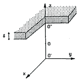
Figure 2: Representation of the changed variable associated with the molecular layer at the solid surface.

b) Calculation of $\displaystyle\ \int\!\!\!\!\int\!\!\!\!\int_{\Omega_{2}}\ m_{1}\ m_{2}\ \chi(r)\ \nu_{2}\ d\omega_{2}$

This term corresponds to the energy with respect to the solid wall.

$$\int\!\!\!\!\int\!\!\!\!\int_{\Omega_{2}}\ m_{1}\ m_{2}\ \chi(r)\ \nu_{2}\ d\omega_{2}\$$

$$=\ m_{1}\ m_{2}\ \nu_{2}\ \int^{2\pi}_{0}\ \bigg{(}\int^{\infty}_{h}\ \chi(r)\ \ \bigg{(}\int^{Arccos\ {h\over r}}_{0}\ \sin\varphi\ d\varphi\bigg{)}r^{2}\ dr\Bigg{)}\ d\theta$$

$$=\ 2\pi\ m_{1}\,m_{2}\,\nu_{2}\int^{\infty}_{h}\ r\ (r-h)\ \chi(r)\ dr$$

which gives relation (7).

Now, we change variable as in Figure 2. The origin of the third coordinate $\ z\$ is placed at $\ 0^{\prime}$. Consequently  $z\ =\ \overline{0^{\prime}0}\$ with $\ 0\$ the position of molecule 1.

If we take now the origin of the $z$-axis at the solid wall and change the orientation in such a way that $\ \overline{00^{\prime\prime}}\ =\ h,\$ we obtain that $\ z+h\$ is a constant for a given molecule. Hence, we get

$${\partial\rho_{1}\over\partial h}\ =\ -\ {\partial\rho_{1}\over\partial z}\ ,\ \ {\partial^{2}\rho_{1}\over\partial h^{2}}\ =\ {\partial^{2}\rho_{1}\over\partial z^{2}}$$

Then,

$$E\ =\ 2\pi\rho^{2}_{1}\ \int^{\infty}_{\sigma}\ r^{2}\ \psi(r)\ dr+\ \pi\rho^{2}_{1}\ \int^{\infty}_{h}\ r(h-r)\ \psi(r)\ dr$$

$$+2\pi\rho_{1}\rho_{2}\ \int^{\infty}_{h}\ r(r-h)\ \chi(r)\ dr+{\pi\over 2}\ \rho_{1}\ {\partial\rho_{1}\over\partial h}\ \int^{\infty}_{h}\ r(h^{2}-r^{2})\ \psi(r)\ dr$$

$$+{\pi\over 3}\rho_{1}\Delta\rho_{1}\ \int^{\infty}_{\sigma}\ r^{4}\ \psi(r)\ dr+{\pi\over 12}\ \rho_{1}\Delta_{T}\rho_{1}\ \int^{\infty}_{h}\Big{(}-2r^{4}+3hr^{3}-rh^{3}\Big{)}\ \psi(r)\ dr$$

$$+{\pi\over 6}\rho_{1}\ {\partial^{2}\rho_{1}\over\partial h^{2}}\ \int^{\infty}_{h}\ r(h^{3}-r^{3})\ \psi(r)\ dr$$

(we note similarly the Laplace operator in new coordinates and in old coordinates). So, we obtain Eq. (8).

Appendix 2.

Some remarks about the potential associated with cohesive forces

In molecular theory it is proved by the virial method than the so-called ”coefficient a” of the van der Waals equation can be obtained from

$$\int^{\infty}_{\sigma}\ \varphi(r)\ 4\pi r^{3}\ dr\ =\ -{6a\over N^{2}}$$

The term $\ \varphi(r)\$ is the magnitude of the attractive force between the two molecules of the fluid at the distance $r,$ and $N$ is the Avogadro number. The potential $\displaystyle\ \psi_{1}(r)\ =\ -\ \int\ \varphi(r)\ dr\$ is assumed to be zero at infinity.

Take the forces in the form

$$\varphi(r)\ ={A\over r^{n}}\ ,\ \ \psi_{1}(r)={A\over(n-1)r^{n-1}}$$

then,

$$4\pi\ A\ \int^{\infty}_{\sigma}\ r^{3-n}\ dr\ =\ {4\pi\ A\ \over n-4}\ {1\over\sigma^{n-4}}$$

and Eq. $(20)$  yields

$$A\ =\ -\ {3(n-4)a\ \sigma^{n-4}\over 2\ \pi\ N^{2}}$$

Let us introduce $\ \psi(r)\$ such that $\displaystyle\ m^{2}_{1}\ \psi(r)\ =\ \psi_{1}(r)$. The term $\ \psi\$ gives the potential per unit mass. Then,

$$\psi(r)\ =\ {-3(n-4)\ a\ \sigma^{n-4}\over 2(n-1)\ \pi\ N^{2}\ m^{2}_{1}\ r^{n-1}}$$

Here,  $Nm\ =\ M\$ denotes the molar mass of the fluid. In case $\ n\ =7\$ (London forces), we get:

$$\psi(r)\ =\ {-3a\ \sigma^{3}\over 4\pi\ M^{2}\ r^{6}}$$

In the following, we use:

$$\psi(r)\ =\ -{k\over r^{6}}\hbox{\hskip 28.45274ptwith \ \ \ }k\ =\ {3a\ \sigma^{3}\over 4\pi\ M^{2}}$$

Consequence: Calculation of $\ E\$ in Eq. (8) for London forces.

Now, using direct integration, we obtain the values of the coefficients given in Eq. (8). Since now

$$\psi(r)\ =\ -\displaystyle{k\over r^{n-1}}\ ,\ \ \ \chi(r)\ =\ -\displaystyle{\mu\over r^{n-1}}\ ,\ \ \ \ \ \hbox{and}\ \ n\ =\ 7$$

we obtain

$$\cases{\ \ \displaystyle 2\pi\ \int^{\infty}_{\sigma}\ r^{2}\ \psi(r)\ dr\ =\ -\ {2\ k\ \pi\over 3\ \sigma^{3}}\cr\cr\cr\ \ \displaystyle{\pi\over 3}\ \int^{\infty}_{\sigma}\ r^{4}\ \psi(r)\ dr\ =\ -\ {k\ \pi\over 3\ \sigma}\cr\cr\cr\ \ \displaystyle 2\ \pi\ \int^{\infty}_{h}\ r\ (r-h)\ \chi(r)\ dr\ =\ -\ {\mu\ \pi\over 6\ h^{3}}\cr\cr\cr\ \ \displaystyle\pi\ \int^{\infty}_{h}\ r\ (h-r)\ \psi(r)\ dr\ =\ {k\ \pi\over 12\ h^{3}}\cr\cr\cr\ \ \displaystyle-\ {\pi\over 2}\int^{\infty}_{h}\ r\ (h^{2}-r^{2})\ \psi(r)\ dr\ =\ -\displaystyle{k\ \pi\over 8\ h^{2}}\cr\cr\cr\ \ \displaystyle{\pi\over 12}\int^{\infty}_{h}\ (-2r^{4}+3h\ r^{3}-r\ h^{3})\ \psi(r)\ dr\ =\ {k\ \pi\over 16\ h}\cr\cr\cr\ \ \displaystyle{\pi\over 6}\int^{\infty}_{h}\ \ r\ (h^{3}-r^{3})\ \psi(r)\ dr\ =\ \ \ \displaystyle{k\ \pi\over 8\ h}}$$

Acknowledgements: I have greatly benefited from generous discussions and correspondence with Professor B. Widom and D${}^{\hbox{r}}$ A. E. van Giessen. Without their interest and help, this paper would be never published. The support of PRC/GdR CNES-CNRS 1185 is gratefully acknowledged.

References

(1) Cahn J. W., J. Chem. Phys., 1977, 66, 3667.

(2) van Giessen A. E., Bukman D. J., Widom B., J. Colloid and Interface Science, 1997, 192, 257.

(3) Zisman W. A., In ”Contact angle, wettability and adhesion”: Advances in Chemistry Series, 43 (Gould R. F., ed.), A.C.S., Washington D. C., 1964, 1.

(4) Li D., Neuman A. W., Langmuir 1993, 9, 3728.

(5) Kwok D. Y., Li D., Neuman A. W., Colloids surfaces, 1994, 89, 181.

(6) Rowlinson J. S., Widom B., Molecular theory of capillarity, Clarendon Press, Oxford, 1984.

(7) Nakanishi H., Fisher M.E., Phys. Rev. Lett., 1982, 49, 1565.

(8) de Gennes P. G., Review of Modern Physics, 1985, 57, 3, 827.

(9) Snook I., van Megen W., J. Chem. Phys., 1979, 70, 3099.

(10) Israelachvili J., Intermolecular and surface forces, Academic Press, London, 1992.

(11) Rocard Y., Thermodynamique, Masson, Paris, 1967, Chapter 5.

(12) Gouin H., Comptes Rendus Acad. Sci. Paris, 1988, 306, II, 755.

(13) de Gennes P. G., J. Phys. (Paris) Lett. 1981, 42, 377.

(14) Fleming P. D., Yang A. J. M., Gibbs J. H. J., Chem. Phys., 1976, 65, 7.