Support Vector Machines and Kd-tree for Separating Quasars from Large Survey Databases

Abstract

We compare the performance of two automated classification algorithms: k-dimensional tree (kd-tree) and support vector machines (SVMs), to separate quasars from stars in the databases of the Sloan Digital Sky Survey (SDSS) and the Two Micron All Sky Survey (2MASS) catalogs. The two algorithms are trained on subsets of SDSS and 2MASS objects whose nature is known via spectroscopy. We choose different attribute combination as input patterns to train the classifier using photometric data only and present the classification results obtained by these two methods. Performance metrics such as precision and recall, true positive rate and true negative rate, F-measure, G-mean and Weighted Accuracy are computed to evaluate the performance of the two algorithms. The study shows that both kd-tree and SVMs are effective automated algorithms to classify point sources. SVMs show slightly higher accuracy, but kd-tree requires less computation time. Given different input patterns based on various parameters(e.g. magnitudes, color information), we conclude that both kd-tree and SVMs show better performance with fewer features. What is more, our results also indicate that the accuracy using the four colors ($u-g$, $g-r$, $r-i$, $i-z$) and $r$ magnitude based on SDSS model magnitudes adds up to the highest value. The classifiers trained by kd-tree and SVMs can be used to solve the automated classification problems faced by the virtual observatory (VO); moreover, they all can be applied for the photometric preselection of quasar candidates for large survey projects in order to optimize the efficiency of telescopes.

1 Introduction

In the recent years, the sizes of astronomical data based on surveys at different wavebands are increasing rapidly. Astronomy has entered a data avalanche era. The most important and challenging issues for the efficient analysis of large multi-wavelength astronomical data rely on data mining tools, which will allow the selection, classification, regression, clustering and even the definition of particular object types within the databases.

Our primary goal is to perform reliable star-quasar separation. Since stars and quasars are point sources, their classification is an important issue in astronomy. In the recent past a lot of work has been carried out on automated approaches. Hatziminaoglou et al. (2000) explored a new joint method (avoiding usual biases) for distinguishing between quasars and stars/galaxies by their photometry. Wolf et al. (2004) explored a photometric method for identifying stars, galaxies and quasars in multi-color surveys. McGlynn (2004) used decision trees to build an online system for automated classification of X-ray sources. Carballo et al. (2004) selected quasar candidates from combined radio and optical surveys using neural networks. Suchkov et al. (2005) applied ClassX, an oblique decision tree classifier optimized for astronomical classification and redshift estimation in the Sloan Digital Sky Survey (SDSS) photometric catalog. Ball et al. (2006) classified stars and galaxies with the SDSS DR3 using decision trees.

In this work we investigate the application of support vector machines (SVMs) and k-dimensional tree (kd-tree) to effectively select quasar candidates. SVMs have been successfully applied in astronomy for mainly the following problems: classification of variable stars (Wozniak et al. 2001, 2004), galaxy morphology classification (Humphreys et al. 2001), solar-flare detection (Qu et al. 2003), classification of multiwavelength data (Zhang & Zhao 2003, 2004), estimation of photometric redshifts of galaxies (Wadadekar 2005; Wang et al. 2007) and matching different object catalogs in astrophysics (Rohde et al. 2005, 2006). Wang et al. (2007) investigated SVMs and Kernel Regression (KR) for photometric redshift estimation with the data from the SDSS Data Release 5 (DR5) and the Two Micron All Sky Survey (2MASS). On the other hand, the kd-tree method is used on the 5 flux-space indexing in the SDSS science archive to partition the bulk data (Kunszt et al. 2000). Maneewongvatana & Mount (2002) presented an empirical analysis of two new splitting methods for kd-trees: sliding-midpoint and minimum-ambiguity, which were designed to remedy some of the deficiencies of the standard kd-tree splitting method, with respect to data distributions that are highly clustered in low-dimensional subspaces. Hsieh et al. (2005) used kd-tree algorithm to divide their sample in order to improve the redshift accuracy of galaxies. Kubica et al. (2007) employed kd-tree for efficient intra- and inter-night linking of asteroid detections. Gao et al. (2008) introduced some application cases of kd-tree in astronomy. In real application, estimation of photometric redshifts belongs to regression problem. Although SVMs and kd-tree are applied for both classification and regression problems, they can’t solve them simultaneously. For classification problem, the predicted parameter is discrete; while for regression problem, the predicted parameter is continuous. When dealing with the two different tasks, the methods should be adjusted.

The structure of this paper is as follows: Section 2 gives the sample collection and parameter selection. Section 3 presents the brief introduction of kd-tree and SVMs. Section 4 illustrates the results and discussion, and the conclusion is presented in Section 5.

2 Sample and Parameter Selection

The Sloan Digital Sky Survey (SDSS, York et al. 2000) uses a dedicated, wide field, 2.5m telescope at Apache Point Observatory, New Mexico. Imaging is carried out in drift-scan mode using a 142 mega-pixel camera in five broad bands, $u$ $g$ $r$ $i$ $z$, spanning the range from 3000 to 10,000$\AA$. The corresponding magnitude limits for the five bands are 22.0, 22.2, 22.2, 21.3 and 20.5, respectively. The Fifth Data Release (DR5) of the SDSS includes all survey quality data taken through June 2005 and represents the completion of the SDSS-I project. It includes five-band photometric data for 215 million unique objects selected over 8000 deg² , and 1,048,960 spectra of galaxies, quasars, and stars selected from 5740 deg² of that imaging data. The magnitude limits for the spectroscopic samples are $r(Petrosian)$=17.77 for the galaxies and $i(PSF)$=19.1 for quasars with redshifts up to 2.3 and $i(PSF)$=20.1 for quasars with higher redshifts.

The Two Micron All Sky Survey (2MASS) project (Cutri et al. 2003) is designed to close the gap between our current technical capability and our knowledge of the near-infrared sky. 2MASS uses two new, highly-automated 1.3m telescopes, one at Mt. Hopkins, AZ, and one at CTIO, Chile. Each telescope is equipped with three-channel camera, each channel consisting of 256x256 array of HgCdTe detectors, capable of observing the sky simultaneously at $J$ (1.25$\mu$m), $H$ (1.65$\mu$m) and $K_{s}$ (2.17$\mu$m), to 3$\sigma$ limiting sensitivity of 17.1, 16.4 and 15.3 mag in the three bands. The number of 2MASS point sources adds up to 470,992,970.

We collected photometric data of quasars and stars with spectra measurement from SDSS DR5, then cross-identified the 2MASS database with these photometric data within a 2 arcsec radius by the federation system of XMaS_VO. XMaS_VO is developed by China-VO project and mainly used for automation of creating databases and cross-identification of catalogues from different bands (Gao et al. 2008). We obtained the samples, as shown in Table 1. The result shows that almost every SDSS object has the counterpart in the 2MASS database and there are only less than 100 missing data records. In our work, for all objects under consideration the SDSS and 2MASS magnitudes are available. In this way the issue of inhomogeneous coverage or non-detections is not dealt with.

Table 1: The number of samples from different catalogs

Catalog	Number of Quasars	Number of Stars
SDSS	76,949	108,744
SDSS+2MASS	76,863	108,679

In order to study the distribution of stars and quasars in the multi-dimensional space, we use different magnitudes: PSF magnitude ($u^{p}$ $g^{p}$ $r^{p}$ $i^{p}$ $z^{p}$), model magnitude ($u$ $g$ $r$ $i$ $z$) and model magnitude with reddening correction ($u^{\prime}$ $g^{\prime}$ $r^{\prime}$ $i^{\prime}$ $z^{\prime}$, hereafter short for dereddened magnitude) from SDSS data, $J$, $H$ and $K_{s}$ magnitudes from 2MASS catalog. The dereddened magnitudes are corrected by Galaxy extinction using the dust maps of Schlegel et al. 1998. $J$, $H$ and $K_{s}$ is the selected “default” magnitude for each band, respectively. If the source is not detected in the band, this is the 95% confidence upper limit derived from a 4 arcsec radius aperture measurement taken at the position of the source on the Atlas Image. We explored different input patterns composed of these attributes.

The mean values of the features selected as input patterns are given in Table 2, which shows the statistical properties of the samples. The first, second and third columns give the number, name and description of the parameters, respectively. The following columns list the mean values of the parameters with standard errors for quasars and stars. Obviously, the mean values of parameters of the samples are different for different classes of objects, especially for the color indexes. Therefore it is reasonable and applicable to discriminate quasars from stars with these features. In order to investigate the distribution of different objects in 2D scatter plots, we randomly select some parameters and subsamples of quasars and stars for visual inspection and plot them in Figure 1.

Taking the pattern ($u-g$, $g-r$, $r-i$, $i-z$, $r$) for example, we apply principal component analysis (PCA) on the sample. PCA is a statistical method that permits the determination of the minimum number of independent or uncorrelated variables underlying a larger number of observed variables (Kendall 1957; Kendall & Stuart 1966). Thus, PCA is used as a technique for both data compression and analysis, in addition, PCA can be used as an unsupervised method for classification. As for PCA used in astronomy, we refer to e.g. Connolly & Szalay (1999 and references therein) or Zhang & Zhao (2003). The result of PCA shows that the first three eigenvectors carry 99.30%, 0.41% and 0.17%, respectively, of the descriptive power. This means that the first three vectors actually carry most of the information, especially the first one. We study the distribution of quasars and stars in the principal component space. To be simple, the subsample randomly selected from the overall sample is shown in Figure 1. PC1, PC2 and PC3 are short for the first, second and third principal components, respectively.

It is obvious from Figure 1 that quasars and stars are not easy to discriminate from each other due to overlapping in the two-color diagrams or the principal component spaces. Therefore we need rely on machine learning or data mining techniques to realize the separation between quasars and stars in the high dimensional space .

Table 2: The mean values of parameters for the samples.

No.	Parameters	Desciption	Quasars	Stars
1 ……	$u^{p}$	SDSS PSF $u$ magnitude	$19.78\pm 1.38$	$20.78\pm 2.57$
2 ……	$g^{p}$	SDSS PSF $g$ magnitude	$19.31\pm 0.89$	$19.32\pm 2.23$
3 ……	$r^{p}$	SDSS PSF $r$ magnitude	$19.06\pm 0.76$	$18.56\pm 1.81$
4 ……	$i^{p}$	SDSS PSF $i$ magnitude	$18.89\pm 0.75$	$18.02\pm 1.51$
5 ……	$z^{p}$	SDSS PSF $z$ magnitude	$18.80\pm 0.76$	$17.73\pm 1.48$
6 ……	$u^{p}-g^{p}$	SDSS PSF $u-g$ color	$0.48\pm 0.79$	$1.46\pm 1.04$
7 ……	$g^{p}-r^{p}$	SDSS PSF $g-r$ color	$0.25\pm 0.35$	$0.76\pm 0.81$
8 ……	$r^{p}-i^{p}$	SDSS PSF $r-i$ color	$0.16\pm 0.20$	$0.54\pm 0.87$
9 ……	$i^{p}-z^{p}$	SDSS PSF $i-z$ color	$0.10\pm 0.18$	$0.30\pm 0.59$
10……	$u$	SDSS model $u$ magnitude	$19.74\pm 1.41$	$20.77\pm 2.63$
11……	$g$	SDSS model $g$ magnitude	$19.23\pm 0.93$	$19.26\pm 2.24$
12……	$r$	SDSS model $r$ magnitude	$18.96\pm 0.84$	$18.49\pm 1.83$
13……	$i$	SDSS model $i$ magnitude	$18.81\pm 0.85$	$17.96\pm 1.52$
14……	$z$	SDSS model $z$ magnitude	$18.71\pm 0.87$	$17.67\pm 1.50$
15……	$u-g$	SDSS model $u-g$ color	$0.50\pm 0.81$	$1.50\pm 1.09$
16……	$g-r$	SDSS model $g-r$ color	$0.26\pm 0.37$	$0.78\pm 0.85$
17……	$r-i$	SDSS model $r-i$ color	$0.17\pm 0.21$	$0.53\pm 0.89$
18……	$i-z$	SDSS model $i-z$ color	$0.10\pm 0.18$	$0.29\pm 0.62$
19……	$u^{\prime}$	SDSS dereddened model $u$ magnitude	$19.58\pm 1.41$	$20.58\pm 2.63$
20……	$g^{\prime}$	SDSS dereddened model $g$ magnitude	$19.12\pm 0.93$	$19.13\pm 2.24$
21……	$r^{\prime}$	SDSS dereddened model $r$ magnitude	$18.89\pm 0.84$	$18.39\pm 1.83$
22……	$i^{\prime}$	SDSS dereddened model $i$ magnitude	$18.74\pm 0.85$	$17.88\pm 1.52$
23……	$z^{\prime}$	SDSS dereddened model $z$ magnitude	$18.87\pm 0.87$	$17.61\pm 1.50$
24……	$u^{\prime}-g^{\prime}$	SDSS dereddened model $u-g$ color	$0.46\pm 0.81$	$1.45\pm 1.09$
25……	$g^{\prime}-r^{\prime}$	SDSS dereddened model $g-r$ color	$0.23\pm 0.37$	$0.74\pm 0.85$
26……	$r^{\prime}-i^{\prime}$	SDSS dereddened model $r-i$ color	$0.15\pm 0.21$	$0.51\pm 0.89$
27……	$i^{\prime}-z^{\prime}$	SDSS dereddened model $i-g$ color	$0.08\pm 0.18$	$0.27\pm 0.62$
28……	$J$	2MASS $J$ magnitude	$15.58\pm 1.39$	$15.39\pm 1.21$
29……	$H$	2MASS $H$ magnitude	$15.00\pm 1.33$	$14.91\pm 1.21$
30……	$K_{s}$	2MASS $K_{s}$ magnitude	$14.67\pm 1.23$	$14.72\pm 1.19$
31……	$J-H$	2MASS $J-H$ color	$0.59\pm 0.27$	$0.48\pm 0.25$
32……	$H-K_{s}$	2MASS $H-K_{s}$ color	$0.32\pm 0.37$	$0.19\pm 0.31$

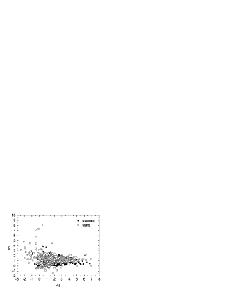
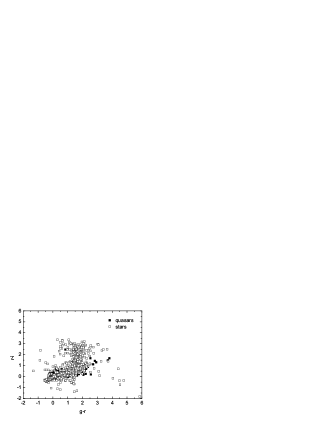
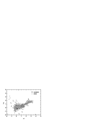
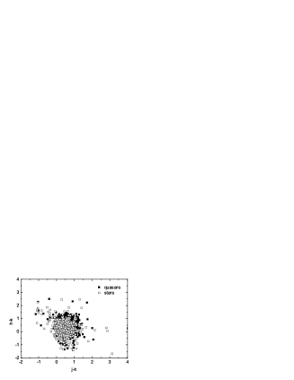
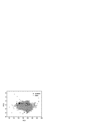
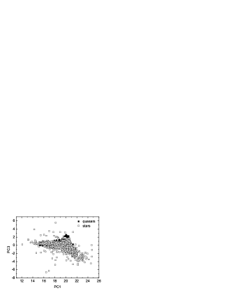
Figure 1: Scatter plots of random subsample (filled squares represent quasars; open ones represent stars.): the upper four diagrams are color-color diagrams; the lower two diagrams are PC1 vs. PC2 and PC1 vs. PC3.

3 The Classification Algorithms

3.1 Kd-tree

K-dimensional tree (kd-tree), as a computer science term, is a space-partitioning data structure for organizing points in a $k$-dimensional space (Bentley, 1975). For more information about kd-tree, we refer to http://en.wikipedia.org/wiki/Kdtree. A kd-tree uses only splitting planes that are perpendicular to one of the coordinate system axes. In addition, in the typical definition every node of a kd-tree, from the root to the leaves, stores a point. As a consequence, each splitting plane must go through one of the points in the kd-tree. Kd-trees are a variant that store data only in leaf nodes. It is worth noting that in an alternative definition of kd-tree the points are stored in its leaf nodes only, although each splitting plane still goes through one of the points. Technically, the letter $k$ refers to the numbers of dimensions. A 3-dimensional kd-tree can be called as 3d-tree. A graphical representation of a 3d-tree is shown in Figure 2. Kd-tree organizes a set of datapoints in k-dimensional space in such a way that once built, whenever a query arrives requesting a list all points in a neighborhood, the query can be answered quickly without needing to scan every single point. Each tree node represents a subvolume of the parameter space, with the root node containing the entire $k$ dimensional volume spanned by the data. Non-leaf nodes have two children, obtained by splitting the widest dimension of the parent’s bounding box, the left child owning those data points that are strictly less than the splitting value in the splitting dimension, and the right child owning the remainder of the parent’s data points. Kd-tree is usually constructed top-down, beginning with the full set of points and then splitting in the center of the widest dimension. This produces two child nodes, each with a distinct set of points. A kd-tree can be constructed by repeating the procedure recursively.

Figure 2: A 3-dimensional kd-tree. The first split (red) cuts the root cell (white) into two subcells, each of which is then split (green) into two subcells. Finally, each of those four is split (blue) into two subcells. Since there is no more splitting, the final eight are called leaf cells. The yellow spheres represent the tree vertices.

3.2 Support Vector Machines

Support vector machines (SVMs) are a set of related supervised learning methods used for classification and regression. SVMs can be considered as a special case of Tikhonov regularization. The idea of SVMs is to map input vectors nonlinearly into a high-dimensional feature space and construct the optimal separating hyperplane in the high-dimensional feature space. SVMs were originally developed by Vapnik (1995), became popular because of many attractive features, and promises empirical performance. SVMs have various parameters that can be tuned for optical performance, including the kernel function. Popular kernels consist of linear, polynomial and radial basis function. SVMs also allow adjusting the soft margin, which is a parameter that controls the trade-off between smooth and overly complex functions. Controlling this trade-off is necessary to obtain good generalization. Functions that represent the training data well but do not generalize to novel examples are said to have overfit the data in machine learning terminology. The soft margin is a tool for SVMs to avoid overfitting (Rohde et al. 2005).

3.3 Performance Measurement

Besides the overall classification accuracy, we use metrics such as true negative rate, true positive rate, Weighted Accuracy (WA), G-mean (GM), precision, recall, and F-measure (FM) to evaluate the performance of classification algorithms (Chen & Liaw 2004). These metrics have been widely used for comparison of different classifiers. All these metrics are functions of the confusion matrix as shown in Table 3. TP is short for the true positive, FN for the false negative, FP for the false positive, TN for the true negative. In the process of classification, quasars are labeled as positive, stars as negative. The rows of the matrix are actual classes, and the columns are the predicted classes. Based on Table 3, the above-mentioned metrics are defined as follows:

$$Accuracy(Acc)={\frac{TP+TN}{TP+FP+TN+FN}}$$ (1)

$$True\ Positive\ Rate(Acc^{+})={\frac{TP}{TP+FN}}=Recall$$ (2)

$$True\ Nagative\ Rate(Acc^{-})={\frac{TN}{TN+FP}}$$ (3)

$$Precision={\frac{TP}{TP+FP}}$$ (4)

$$F-measure(FM)={\frac{2\times{Precision\times{Recall}}}{Precision+Recall}}$$ (5)

$$G-mean(GM)=(Acc^{-}\times{Acc^{+}})^{\frac{1}{2}}$$ (6)

$$Weighted\ Accuracy(WA)=\beta\times{Acc^{+}}+(1-\beta)\times{Acc^{-}}$$ (7)

Table 3: Confusion matrix.

	Predicted Positive Class	Predicted Negative Class
Actual Positive class	TP (True Positive)	FN (False Negative)
Actual Negative class	FP (False Positive)	TN (True Negative)

Recall is the fraction of actual positive cases that were correct, and precision is the fraction of the predicted positive cases that were correctly identified. For any classifier, there is always a trade off between recall and precision. The Geometric Mean (G-mean) is useful to determine “average factors”. The F-measure can be interpreted as a weighted average of the precision and recall. Weighted Accuracy uses an adjusted parameter $\beta$ to suit different applications. Here we use equal weights for both true positive rate and true negative rate; i.e., $\beta$ equals 0.5. These metrics are commonly used in the information retrieval area as performance measures. We will adopt all these measurements to compare our methods with different patterns. Train-test and ten-fold cross-validation were carried out to obtain all the performance metrics.

4 RESULTS AND DISCUSSION

Our experiments are performed using the kd-tree java package (http://www.cs.wlu.edu/ levy/software/kd/) written by Simon D. Levy and SVMLight which is an implementation of SVMs in C language (http://svmlight.joachims.org/). The configuration of the PC computer used was Microsoft Windows XP, Pentium (R) 4, 3.2 GHz CPU, 1.00 GB memory. One advantage of the empirical training set approach to classification is that additional parameters can be easily incorporated. More parameters may be taken as inputs. In order to study which parameters influence the classification accuracy, we probe different input patterns to separate quasars from stars. We compare the performance of kd-tree and SVMs with different input patterns. Our experiment results are shown in Tables 4-8. We calculate accuracy, true positive rate, true negative rate, precision, F-measure, G-mean, Weighted Accuracy and running time for all experiment results. We apply these criteria to determine which pattern is best. Here we take quasars as the positive class and stars as the negative one. For Weighted Accuracy, we adopt equal weights for both true positive rate and true negative rate ($\beta$ equals 0.5).

4.1 Results of kd-tree

Firstly, we explore kd-tree to isolate quasars from stars with different input patterns. Each of the samples is randomly divided into two parts: two thirds for training a classifier and one third for testing the classifier to get the classification rate. This method is usually called train-test method. For different input patterns, the number of samples is different. The label $Q$ ($Q$ for quasars) or $S$ ($S$ for stars) as input index is inserted into the samples and used to build a kd-tree classifier in a supervised way. Then we use the test samples to get the optimal value of $n$ nearest neighbors. For each test sample, we need judge if there are more than half of the $n$ nearest neighbors which are equal to the test sample’s input index to obtain correct or incorrect prediction. So the $n$ value must be an odd integer to avoid half-and-half case. In theory, the higher values of $n$ provide smoothing that reduces vulnerability to noise in the training data. In practical applications $n$ is typically in units or tens rather than in hundreds or thousands. We set $n$=11 for this experiment because of its higher accuracy. The magnitudes in five bands ($u$, $g$, $r$, $i$, $z$) are taken as the first set of input parameters for kd-tree, and then the four color index ($u-g$, $g-r$, $r-i$, $i-z$) and $r$ magnitude are as input patterns. There will be more information for classification if more parameters are included. $J$, $H$ and $K_{s}$ magnitudes (or $J-H$ and $H-K_{s}$) from 2MASS catalog are added as extra inputs to build our classifier. We compare the performance of different input patterns based on PSF magnitudes, model magnitudes and dereddened magnitudes. The comparison of different input patterns are listed in Table 4.

Table 4 shows that for any input patterns using kd-tree method, the accuracy is rather high, more than 94.47%, with high values of F-measure, G-mean and Weighted Accuracy, and the running time is less than 5 minutes. Generally, the performance of similar input patterns based on model magnitudes adds up to a higher accuracy than those based on other kinds of magnitudes, those of dereddened magnitudes are better than those of PSF magnitudes. For these three kinds of magnitudes, the results based on four colors and $r$ magnitude as input patterns outperform those of the five magnitudes. The accuracy does not always increase with more features considered, for example, the accuracy seems to decrease when the input patterns given parameters $J$, $H$, $K_{s}$, or $J-H$, $H-K_{s}$. Only when appropriate features adopted, the performance is best. In the situations of fewer features, kd-tree shows better performance and uses less building time. As shown by Table 4, the four model color index ($u-g$, $g-r$, $r-i$, $i-z$) and the model $r$ magnitude as the input pattern obtains the highest accuracy which amounts to 97.26%, and the highest value of F-measure, G-mean and Weighted Accuracy which are 96.69%, 97.14% and 97.14%, respectively, moreover the running time is shorter, not more than 1 minute.

Table 4: The comparison of different input patterns using kd-tree when $n$=11.

Input patterns	Acc	Acc+	Acc-	Precision	FM	GM	WA	Time
	(%)	(%)	(%)	(%)	(%)	(%)	(%)	(s)
$u^{p},g^{p},r^{p},i^{p},z^{p}$	$96.32$	$95.34$	$97.02$	$95.76$	$95.55$	$96.17$	$96.18$	$27$
$u^{p}-g^{p},g^{p}-r^{p},r^{p}-i^{p},i^{p}-z^{p},r^{p}$	$97.02$	$96.24$	$97.58$	$96.56$	$96.40$	$96.90$	$96.91$	$48$
$u^{p},g^{p},r^{p},i^{p},z^{p},J-H,H-K_{s}$	$95.82$	$94.90$	$96.48$	$95.01$	$94.96$	$95.69$	$95.69$	$83$
$u^{p}-g^{p},g^{p}-r^{p},r^{p}-i^{p},i^{p}-z^{p},r^{p},J-H,H-K_{s}$	$96.62$	$95.89$	$97.14$	$95.96$	$95.92$	$96.51$	$96.52$	$166$
$u^{p},g^{p},r^{p},i^{p},z^{p},J,H,K_{s}$	$94.81$	$93.91$	$95.45$	$93.58$	$93.75$	$94.67$	$94.68$	$90$
$u^{p}-g^{p},g^{p}-r^{p},r^{p}-i^{p},i^{p}-z^{p},r^{p},J,H,K_{s}$	$95.76$	$95.08$	$96.24$	$94.70$	$94.89$	$95.66$	$95.66$	$166$
$u,g,r,i,z$	$96.46$	$95.42$	$97.20$	$96.02$	$95.72$	$96.31$	$96.31$	$26$
u-g,g-r,r-i,i-z,r	97.26	$96.41$	$97.87$	$96.97$	96.69	97.14	97.14	$54$
$u,g,r,i,z,J-H,H-K_{s}$	$95.85$	$94.90$	$96.53$	$95.09$	$94.99$	$95.71$	$95.72$	$91$
$u-g,g-r,r-i,i-z,r,J-H,H-K_{s}$	$96.76$	$96.02$	$97.28$	$96.15$	$96.08$	$96.65$	$96.65$	$148$
$u,g,r,i,z,J,H,K_{s}$	$94.87$	$93.88$	$95.57$	$93.75$	$93.81$	$94.72$	$94.73$	$91$
$u-g,g-r,r-i,i-z,r,J,H,K_{s}$	$95.85$	$95.09$	$96.39$	$94.90$	$95.00$	$95.74$	$95.74$	$167$
$u^{\prime},g^{\prime},r^{\prime},i^{\prime},z^{\prime}$	$96.41$	$95.42$	$97.10$	$95.88$	$95.65$	$96.26$	$96.26$	$25$
$u^{\prime}-g^{\prime},g^{\prime}-r^{\prime},r^{\prime}-i^{\prime},i^{\prime}-z^{\prime},r^{\prime}$	$97.19$	$96.37$	$97.76$	$96.82$	$96.60$	$97.07$	$97.07$	$44$
$u^{\prime},g^{\prime},r^{\prime},i^{\prime},z^{\prime},J-H,H-K_{s}$	$95.8$	$95.00$	$96.47$	$95.01$	$95.00$	$95.73$	$95.74$	$81$
$u^{\prime}-g^{\prime},g^{\prime}-r^{\prime},r^{\prime}-i^{\prime},i^{\prime}-z^{\prime},r^{\prime},J-H,H-K_{s}$	$96.68$	$95.97$	$97.18$	$96.00$	$95.99$	$96.57$	$96.57$	$151$
$u^{\prime},g^{\prime},r^{\prime},i^{\prime},z^{\prime},J,H,K_{s}$	$94.73$	$93.78$	$95.41$	$93.52$	$93.65$	$94.59$	$94.59$	$89$
$u^{\prime}-g^{\prime},g^{\prime}-r^{\prime},r^{\prime}-i^{\prime},i^{\prime}-z^{\prime},r^{\prime},J,H,K_{s}$	$95.76$	$95.04$	$96.27$	$94.74$	$94.89$	$95.65$	$95.65$	$178$

From the above results, we conclude that the four model colors ($u-g$, $g-r$, $r-i$, $i-z$) and the model $r$ magnitude is the best input pattern for kd-tree when setting $n=11$. Now we adopt such pattern as input pattern and investigate the influence of the $n$ value on the performance of kd-tree. We change the value of $n$ for different experiments. By comparing accuracy, F-measure, G-mean and Weighted Accuracy of classification and the running time taken to build a classifier, we estimate the efficiency and effectiveness of the classifiers created by different $n$ values in the experiments. Through the attempts, we obtain the optimal $n$ value of nearest neighbors. Here we adopt the odd integer of $n$ from 3 to 29 in our experiments. Table 5 indicates that the highest accuracy of classification is 97.263% when $n$=11, and the next highest results are 97.262% and 97.252% when $n$=7 and $n$=9, respectively. The running time is longer when the value of $n$ is bigger in our experiment. As $n$=7, the simultaneous highest values of F-measure, G-mean and Weighted Accuracy are 96.690%, 97.149% and 97.151%, respectively. We also see that the true positive rate is higher for $n$=7 than for $n$=9 or 11, which means that the classifier we build using $n$=7 gives high prediction accuracy over the quasar class, while maintaining reasonable accuracy for the star class.

Table 5: The comparison of different $n$ value for kd-tree with four model colors ($u-g$, $g-r$, $r-i$, $i-z$) and model $r$ magnitude as input pattern.

$n$	Acc	Acc+	Acc-	Precision	FM	GM	WA	Time
	(%)	(%)	(%)	(%)	(%)	(%)	(%)	(s)
3	$97.167$	$96.479$	$97.654$	$96.677$	$96.578$	$97.065$	$97.066$	$29$
5	$97.239$	$96.554$	$97.723$	$96.775$	$96.665$	$97.137$	$97.139$	$35$
7	97.262	$96.503$	$97.799$	$96.877$	96.690	97.149	97.151	$41$
9	$97.252$	$96.452$	$97.818$	$96.902$	$96.677$	$97.133$	$97.135$	$46$
11	97.263	$96.413$	$97.866$	$96.966$	$96.689$	$97.137$	$97.140$	$50$
13	$97.228$	$96.412$	$97.804$	$96.882$	$96.646$	$97.106$	$97.108$	$54$
15	$97.187$	$96.342$	$97.785$	$96.853$	$96.597$	$97.061$	$97.064$	$57$
17	$97.130$	$96.227$	$97.768$	$96.826$	$96.526$	$96.994$	$96.998$	$61$
19	$97.102$	$96.153$	$97.774$	$96.831$	$96.491$	$96.960$	$96.964$	$64$
21	$97.081$	$96.149$	$97.740$	$96.785$	$96.466$	$96.941$	$96.945$	$67$
23	$97.064$	$96.113$	$97.737$	$96.780$	$96.445$	$96.922$	$96.925$	$70$
25	$97.043$	$96.082$	$97.723$	$96.760$	$96.420$	$96.899$	$96.903$	$73$
27	$97.004$	$96.023$	$97.698$	$96.724$	$96.372$	$96.857$	$96.861$	$76$
29	$96.968$	$95.956$	$97.684$	$96.702$	$96.328$	$96.816$	$96.820$	$78$

4.2 Results of SVMs

Since the best input pattern is four model colors ($u-g$, $g-r$, $r-i$, $i-z$) and model $r$ magnitude for kd-tree, we apply such input pattern to create the SVM classifier. The kernel function of SVMs we choose is the radial basis function (RBF). When using RBF SVMs, there are two adjusted parameters: $\gamma$ is the parameter in RBF kernel and $c$ is the trade-off between training error and margin. Here we try to compare the classifier created by the different values of these two parameters in our experiments, and the results are listed in Table 6. It can be seen that the best accuracy (97.50%) is obtained using RBF SVM classifier with $\gamma$=5 and $c$=1 or 5 and the building time is 21 min and 28 min, respectively. However, the highest F-measure value is 97.78% with $\gamma$=8 and $c$=1, and the highest values of G-mean and Weighted Accuracy are 97.41% and 97.41% with $\gamma$=5 and $c$=5. We also find that the true positive rate when $\gamma$=5 and $c$=5 is superior to that when $\gamma$=5 and $c$=1, but the former takes more training time. Table 6 shows that in the situation of the smaller $c$ value, less running time is generally taken. So when $\gamma$ equals 5 and $c$ equals 0.1, we take the least time to build the SVM classifier, while $\gamma$ equals 0.01 and $c$ equals 1000, the time taken adds up to 1 day and 14 hours.

On account of the highest values of G-mean and Weighted Accuracy in Table 6, the optimal values of $\gamma$ and $c$ are 5 for RBF SVMs. Then setting $\gamma$=5 and $c$=5, we compute accuracy, true positive rate, true negative rate, precision, F-measure, G-mean and Weighted Accuracy for different input patterns using RBF SVMs in Table 7. Clearly based on accuracy, F-measure, G-mean and Weighted Accuracy, the input pattern of ($u-g$, $g-r$, $r-i$, $i-z$, $r$) is the optimal pattern. Using four colors and $r$ magnitude ($u-g$, $g-r$, $r-i$, $i-z$, $r$) as input pattern, the performance of SVMs is better than the five magnitudes ($u$, $g$, $r$, $i$, $z$). Similar to the result of kd-tree, the performance based on the model magnitudes outperforms that based on the dereddened magnitudes, which is superior to that based on the PSF magnitudes. When adding more parameters from near infrared band, the performance doesn’t improve, even decrease. This shows that $J-H$ and $H-K_{s}$ contribute little information for classification.

Table 6: The comparison of different options using RBF SVMs with four model colors ($u-g$, $g-r$, $r-i$, $i-z$) and model $r$ magnitude as input pattern.

Algorithm	Soft margin	Acc	Acc+	Acc-	Precision	FM	GM	WA	Time
(RBF kernel)	$c$	(%)	(%)	(%)	(%)	(%)	(%)	(%)	(m)
$\gamma=5$	$c=0.1$	$96.85$	$95.14$	$98.07$	$97.22$	$97.64$	$96.59$	$96.60$	$17$
$\gamma=0.01$	$c=1$	$92.09$	$88.69$	$94.50$	$91.95$	$93.21$	$91.55$	$91.60$	$32$
$\gamma$=5	c=1	97.50	$96.67$	$98.09$	$97.27$	$97.68$	$97.38$	$97.38$	$21$
$\gamma=8$	$c=1$	$97.48$	$96.50$	$98.17$	$97.39$	97.78	$97.33$	$97.34$	$30$
$\gamma=0.01$	$c=10$	$92.90$	$89.37$	$95.40$	$93.22$	$94.30$	$92.34$	$92.39$	$47$
$\gamma=5$	$c=10$	$97.41$	$96.86$	$97.79$	$96.88$	$97.33$	$97.32$	$97.33$	$69$
$\gamma$=5	c=5	97.50	$96.88$	$97.93$	$97.07$	$97.50$	97.41	97.41	$49$
$\gamma=8$	$c=5$	$97.38$	$96.61$	$97.92$	$97.04$	$97.48$	$97.26$	$97.26$	$54$
$\gamma=0.01$	$c=1000$	$94.55$	$94.26$	$96.02$	$92.47$	$93.60$	$94.50$	$94.50$	$2280$

Table 7: The comparison of different input patterns using RBF SVM when $c$=5 and $\gamma$=5.

Input patterns	Acc	Acc+	Acc-	Precision	FM	GM	WA	Time
	(%)	(%)	(%)	(%)	(%)	(%)	(%)	(m)
$u^{p},g^{p},r^{p},i^{p},z^{p}$	$96.97$	$96.47$	$97.40$	$96.97$	$97.19$	$96.94$	$96.94$	$58$
$u^{p}-g^{p},g^{p}-r^{p},r^{p}-i^{p},i^{p}-z^{p},r^{p}$	$97.39$	$96.95$	$97.77$	$97.39$	$97.58$	$97.36$	$97.36$	$42$
$u,g,r,i,z$	$97.15$	$96.64$	$97.59$	$97.16$	$97.37$	$97.11$	$97.11$	$61$
u-g,g-r,r-i,i-z,r	97.50	$96.97$	$97.93$	$97.49$	97.71	97.45	97.45	$44$
$u-g,g-r,r-i,i-z,r,J-H,H-K_{s}$	$97.17$	$96.16$	$97.93$	$97.18$	$97.55$	$97.04$	$97.04$	$62$
$u^{\prime},g^{\prime},r^{\prime},i^{\prime},r^{\prime}$	$97.15$	$96.72$	$97.53$	$97.16$	$97.34$	$97.12$	$97.12$	$60$
$u^{\prime}-g^{\prime},g^{\prime}-r^{\prime},r^{\prime}-i^{\prime},i^{\prime}-z^{\prime},r^{\prime}$	$97.47$	$97.02$	$97.85$	$97.47$	$97.66$	$97.44$	$97.44$	$43$

Finally, we use 10-fold cross-validation to evaluate the performance and the speed to build the classifiers of kd-tree and SVMs and adopt the four colors ($u-g$, $g-r$, $r-i$, $i-z$) and $r$ magnitude as input pattern in order to compare their performance. Cross-validation is a generally applicable and very useful technique for many tasks often encountered in machine learning, such as accuracy estimation, feature selection or parameter tuning. Cross-validation is used within a wide range of machine learning approaches, such as kd-tree and SVMs. K-fold cross-validation is an important cross-validation method applicable for data set with moderate size. The data is randomly partitioned into $k$ subsamples. Each time, one of the subsamples is retained as the testing data, and the remaining $k-1$ subsamples are put together to form the training data. The cross-validation process is then repeated $k$ times, then the mean error and the evaluated value across all trials is computed. The comparison of the efficiency and effectiveness of the two methods is based on the metrics such as true negative rate, true positive rate, Weighted Accuracy, G-means, precision, recall, and F-measure to evaluate the performance of learning algorithms.

Given the metrics in Table 8, the best results only with respect to accuracy is obtained using RBF SVM classifier with $\gamma$=5 and $c$=5, when the accuracy of classification is 97.65% and the standard error is 0.22%. Furthermore, we get the accuracy of 97.65% when $\gamma$=2 and $c$=10, and 97.64% when $\gamma$=5 and $c$=1, but the standard error of the latter is the smallest among these three best cases. The highest F-measure is 98.01% with $\gamma$=10 and $c$=1; the highest G-mean and Weighted Accuracy value are 97.55% and 97.56%. Kd-tree obtains the best result when $n$=9. The highest values of accuracy, F-measure, G-mean and Weighted Accuracy amounts to 97.45%, 97.66%, 97.32% and 97.32%, respectively, and these results are a little better than those when $n$=11. Clearly based on the metrics in Table 8, we can hardly tell the difference between kd-tree and SVMs. SVMs is slightly better than kd-tree in G-mean, F-measure and Weighted Accuracy. Since the accuracy of the two learning algorithms is more than 97.0%, the two methods are effective classifiers to isolate quasars from stars.

4.3 Performance Comparison of kd-tree and SVMs

From the tables above we conclude that kd-tree and SVMs are comparable to separate quasars from stars in respect of the accuracy. When only considering the running time, kd-tree is much faster than SVMs, for the speed of kd-tree is measured by seconds while that of SVMs is measured by minutes, as shown in Tables 4-7. Taking into account both accuracy and speed, kd-tree shows its superiority, because the speed to build the SVM classifier is very slow. Moreover, the performance obtained by the 10-fold cross-validation method gets higher accuracy than the train-test method because the cross-validation method has the advantage of producing an effectively unbiased error estimate, but it is computationally expensive (about 10 times longer than train-test method). As a result, the classifiers trained with kd-tree and SVMs can be used to classify the unclassified sources and be applicable to preselect quasar candidates from SDSS and other survey catalogs.

Table 8: The comparison of different $n$ or ($\gamma$ and $c$) using 10-fold cross-validate method with four model colors ($u-g$, $g-r$, $r-i$, $i-z$) and model $r$ magnitude as input pattern.

$n$/($\gamma,c$)	Acc	Acc+	Acc-	Precision	FM	GM	WA
	(%)	(%)	(%)	(%)	(%)	(%)	(%)
$n=13$	$97.40\pm 0.23$	$96.47\pm 0.31$	$98.06\pm 0.34$	$97.24\pm 0.48$	$97.65\pm 0.41$	$97.26\pm 0.23$	$97.26\pm 0.23$
$n=11$	$97.42\pm 0.25$	$96.53\pm 0.31$	$98.06\pm 0.35$	$97.24\pm 0.48$	$97.65\pm 0.41$	$97.29\pm 0.24$	$97.29\pm 0.24$
n=9	97.45$\pm$0.23	$96.58\pm 0.28$	$98.07\pm 0.34$	$97.26\pm 0.47$	97.66$\pm$0.41	97.32$\pm$0.22	97.32$\pm$0.22
$n=7$	$97.44\pm 0.23$	$96.60\pm 0.30$	$98.03\pm 0.34$	$97.21\pm 0.47$	$97.62\pm 0.41$	$97.31\pm 0.22$	97.32$\pm$0.22
c=1, $\gamma$=5	97.64$\pm$0.20	$96.76\pm 0.26$	$98.26\pm 0.34$	$97.52\pm 0.47$	$97.89\pm 0.40$	$97.50\pm 0.19$	$97.51\pm 0.19$
$c=1$,$\gamma$=8	$97.62\pm 0.21$	$96.64\pm 0.22$	$98.31\pm 0.33$	$97.59\pm 0.46$	$97.95\pm 0.40$	$97.47\pm 0.19$	$97.47\pm 0.19$
$c=1$,$\gamma$=10	$97.59\pm 0.22$	$96.50\pm 0.26$	$98.37\pm 0.34$	$97.66\pm 0.48$	98.01$\pm$0.41	$97.43\pm 0.21$	$97.43\pm 0.21$
$c=1$,$\gamma$=2	$97.46\pm 0.19$	$96.63\pm 0.26$	$98.04\pm 0.32$	$97.22\pm 0.43$	$97.63\pm 0.38$	$97.33\pm 0.17$	$97.34\pm 0.17$
c=5, $\gamma$=5	97.65$\pm$0.22	$96.97\pm 0.24$	$98.14\pm 0.35$	$97.37\pm 0.35$	$97.75\pm 0.42$	97.55$\pm$0.20	97.56$\pm$0.20
$c=5$,$\gamma$=8	$97.61\pm 0.26$	$97.40\pm 0.28$	$98.17\pm 0.39$	$97.40\pm 0.54$	$97.78\pm 0.46$	$97.49\pm 0.24$	$97.50\pm 0.24$
$c=5$,$\gamma$=10	$97.54\pm 0.26$	$96.66\pm 0.31$	$98.17\pm 0.37$	$97.39\pm 0.52$	$97.78\pm 0.45$	$97.41\pm 0.25$	$97.41\pm 0.25$
$c=10$,$\gamma$=5	$97.61\pm 0.26$	$96.96\pm 0.27$	$98.07\pm 0.41$	$97.27\pm 0.56$	$97.67\pm 0.48$	$97.51\pm 0.24$	$97.51\pm 0.24$
$c=10$,$\gamma$=8	$97.50\pm 0.26$	$96.74\pm 0.30$	$98.03\pm 0.40$	$97.20\pm 0.55$	$97.61\pm 0.48$	$97.38\pm 0.25$	$97.39\pm 0.25$
$c=10$,$\gamma$=10	$97.40\pm 0.25$	$96.53\pm 0.32$	$98.02\pm 0.36$	$97.19\pm 0.50$	$97.60\pm 0.43$	$97.27\pm 0.24$	$97.28\pm 0.24$
c=10,$\gamma$=2	97.65$\pm$0.22	$97.00\pm 0.28$	$98.10\pm 0.35$	$97.31\pm 0.49$	$97.70\pm 0.42$	97.55$\pm$0.20	$97.55\pm 0.20$

The sources inclined to be misclassified due to their intrinsic properties are equally prone to misclassification wether kd-tree or SVMs is used. Most of the sources misclassified by kd-tree overlap those misclassified by SVMs, as proved by the experimental results. In order to visualize the classification results, we take the kd-tree method as an example. In Figure 3, we plot the quasars and misclassified quasars as the function of redshifts. Figure 3 shows that the peak of the quasar sample lies in the redshift range 1 to 2, while the peak of misclassified quasars lies in the range 2.5 to 4. The highest peak of the redshift distribution for misclassified quasars occurs at z$\sim$2.8, which is exactly the redshift range in which the distinction between M stars and quasars becomes problematic when the Sloan photometric system is used. The misclassification simply indicates that, no matter what the classification method is, one is prone to the same biases because of the very nature of objects. That the peak of misclassified quasars’ $r$-band magnitude is faint is again due to the fact that the magnitude limit of the spectroscopic sample was fainter for higher redshift objects. In addition, we investigate the classified result as the function of magnitude, as shown in Figure 4. From Figure 4, it is obviously found that the peak of misclassified quasars or stars (right panel in Figure 3) shifts to the faint magnitude compared to quasars and stars (left panel in Figure 3). In other words, the faint sources are inclined to be misclassified, which possibly results from the small sample size and low S/N ratio for these faint sources. We further want to know why the misclassified sources are prone to be misclassified, so we consult the misclassified quasars and stars from SIMBAD astronomical database and NASA/IPAC Extragalactic Database (NED). Of the misclassified stars, the most objects are CV stars, white dwarfs, RR star, carbon stars, some objects are ultra-violet sources, X-ray sources, radio sources, blue sources, and HII region, some objects are galaxies and irregular spirals, a few are quasars. Of 893 misclassified quasars, most are quasars with faint magnitudes, some are AGN, Seyfert 1, Seyfert 2, damped Lyman absorbtion and radio sources, a part are 171 unidentified quasars, and the little part are 4 white dwarfs, one CV star, one AM star and 29 galaxies.

Figure 3: The distribution of quasars and misclassified quasars as a function of redshift $Z$.

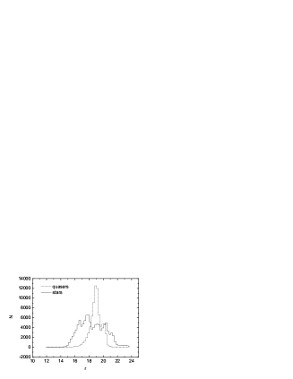
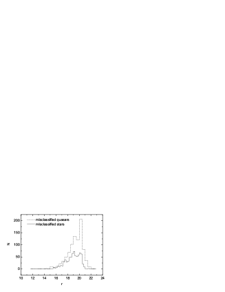
Figure 4: The distribution of quasars and misclassified quasars (dotted line) as well as stars and misclassified stars (solid line) as a function of model $r$ magnitude.

5 CONCLUSION

In this paper we have investigated k-dimensional tree (kd-tree) and support vector machines (SVMs) applied to the datasets from optical and infrared band catalogs (SDSS DR5 and 2MASS), and tested it with different input patterns. We have computed the performance metrics such as precision and recall, true positive rate and true negative rate, F-measure, G-mean and Weighted Accuracy to evaluate the performance of learning algorithms. Based on these metrics from the results by kd-tree and SVMs, we can not tell clearly which is superior. Kd-tree and SVMs are comparable to separate quasars from stars only considering the accuracy. Nevertheless, kd-tree is much faster to create a classifier than SVMs with respect to the speed. In real applications, there is one parameter (e.g. the number of neighbors) to adjust in the kd-tree method while there are two adjusted parameters (e.g. $\gamma$ and $c$) to control in the SVM approach when using RBF kernel function. Therefore it is not easy to modulate optimal parameters and get good performance for SVMs. Given high accuracy, fast speed and easy modulation of parameters, kd-tree may be a good choice for classification. Furthermore, both kd-tree and SVMs show better performance when considering fewer input parameters. Among the input patterns based on the three kinds of SDSS magnitudes, the performance of the model magnitudes is the best and that of the dereddened magnitudes is better than that of the PSF magnitudes. The input patterns of four colors and $r$ magnitude ($u-g$, $g-r$, $r-i$, $i-z$, $r$) gets better performance than the five magnitudes ($u$, $g$, $r$, $i$, $z$). We consider more parameters from 2MASS catalog as extra inputs to our classifiers, but the results are not better, which is possible attributed to the bright magnitude limit of $J$, $H$, $K_{s}$; however other issues might cause this effect, such as the low measurement precision of magnitudes. In the experiments, we employ the train-test method and 10-fold cross-validation method to create classifiers. The results show that the cross-validation method is superior to the train-test method because the former method avoids the random selection of sample. When the data are complete or the quality and quantity of data further improve, the performance of classifiers will improve. These two approaches can be used to solve the classification problems faced in astronomy. These classifiers trained by these methods can be used to classify sources with multi-wavelength astronomical data and preselect quasar candidates for large surveys, such as the Chinese Large Sky Area Multi-Object Fiber Spectroscopic Telescope (LAMOST). Moreover the two methods may be integrated into the data mining toolkit of Virtual Observatories.

6 ACKNOWLEDGMENTS

We are very grateful to referee’s constructive and insightful suggestions as well as helping us improve writing. We would like to thank LAMOST staff for their help. This paper is funded by National Natural Science Foundation of China under grant under Grant Nos. 10473013, 90412016 and 10778724. This research has made use of data products from the SDSS survey and from the Two Micron All Sky Survey (2MASS). The SDSS is managed by the Astrophysical Research Consortium for the Participating Institutions. The Participating Institutions are the American Museum of Natural History, Astrophysical Institute Potsdam, University of Basel, University of Cambridge, Case Western Reserve University, University of Chicago, Drexel University, Fermilab, the Institute for Advanced Study, the Japan Participation Group, Johns Hopkins University, the Joint Institute for Nuclear Astrophysics, the Kavli Institute for Particle Astrophysics and Cosmology, the Korean Scientist Group, the Chinese Academy of Sciences (LAMOST), Los Alamos National Laboratory, the Max-Planck-Institute for Astronomy (MPIA), the Max-Planck-Institute for Astrophysics (MPA), New Mexico State University, Ohio State University, University of Pittsburgh, University of Portsmouth, Princeton University, the United States Naval Observatory, and the University of Washington. 2MASS is a joint project of the University of Massachusetts and the Infrared Processing and Analysis Center/California Institute of Technology, funded by the National Aeronautics and Space Administration and the National Science Foundation. This research has made use of the NASA/IPAC Extragalactic Database (NED) which is operated by the Jet Propulsion Laboratory, California Institute of Technology, under contract with the National Aeronautics and Space Administration. This research has also made use of the SIMBAD database, operated at CDS, Strasbourg, France.

References

- [1] Ball, N. M., Brunner, R. J., Myers, A. D., Tcheng, D., 2006, ApJ, 650, 497
- [2] Bentley, J. L., 1975, Commun. ACM 18, 9 (Sep. 1975), 509
- [3] Carballo, R., Cofio, A. S., Gonzlez-Serrano, J. I., 2004, MNRAS, 353, 211
- [4] Chen, C., Liaw, A., 2004, Department of Stastics, UC Berkeley, Technical Report, 666
- [5] Connolly, A. J., Szalay, A. S., 1999, AJ, 117, 2052
- [6] Cutri, R. M., Skrutskie, M. F., van Dyk, S., Beichman, C. A., Carpenter, J. M., Chester, T., Cambresy, L., Evans, T. et al., 2003, The IRSA 2MASS All-Sky Point Source Catalog, NASA/IPAC Infrared Science Archive
- [7] Gao, D., Lu, Y., Zhang, Y., Zhao, Y., 2008, Astronomical Research & Techonolgy-Publications of National Astronomical Observatories of China, accepted
- [8] Gao, D., Zhang, Y., Zhao, Y., 2008, astro-ph/08012004
- [9] Hatziminaoglou, E., Mathez, G., Pell, R., 2000, A&A. 359, 9
- [10] Hsieh, B. C., Yee, H. K. C., Lin, H., 2005, ApJs, 158(2), 161
- [11] Humphreys, R. M., Karypis, G., Hasan, M., Kriessler, J., Odewahn, S. C., 2001, American Astronomical Society, 33, 1322
- [12] Kendall, M. G., 1957, A Course of Multivariate Analysis (London: Griffin & Co.)
- [13] Kendall, M. G., Stuart, A., 1996, in Advanced Theory of Statistics, Vol. 3 (London: Griffin & Co), 285
- [14] Kubat, M., Matwin, S., 1997, In Proceedings of the 14th International conference on Machine Learning, 179
- [15] Kubica, J., Denneau, L., Grav, T., Heasley, J., Jedicke, R., Masiero, J., Milani, A., Moore, A,. et al., 2007, Icarus, 189(1), 151
- [16] Kunszt, P. Z., Szalay, A. S., Csabai, I., Thakar, A. R., 2000, ASPC, 216, 141
- [17] Maneewongvatana, S., Mount, D. M., 2002, DIMACS Series in Discrete Mathematics and Theoretical Computer Science, 59, 105
- [18] McGlynn, T. A., Suchkov, A. A., Winter, E. L., Hanisch, R. J., White, R. L., Ochsenbein, F., Derriere, S., Voges, W. et al., 2004, ApJ, 616
- [19] Monet, D. G., Levine, S. E., Casian, B., Ables, H. D., Bird, A. R., Dahn, C. C., Guetter, H. H., Harris, H. C. et al., 2003, AJ, 125, 984
- [20] Qu, M., Shih, F. Y., Jing, J., Wang, H. M., 2003, Solar Physics, 217(1), 157
- [21] Rohde, D. J., Drinkwater M. J., Gallagher M. R., Downs, T., Doyle, M. T., 2005, MNRAS, 360, 69
- [22] Rohde, D. J., Gallagher, M. R., Drinkwater, M. J., Pimbblet, K. A., 2006, MNRAS, 369, 2
- [23] Schlegel, D. J., Finkbeiner, D. P., Davix, M., 1998, ApJ, 500, 525
- [24] Suchkov, A. A., Hanisch, R. J., Margon, Bruce., 2005, AJ, 130, 2439
- [25] Thorsten Joachims, Learning to Classify Text Using Support Vector Machines., 2002, Dissertation, Kluwer
- [26] Vapnik, V. N., 1995, The Nature of Statistical Learning Theory (New York: Springer)
- [27] Wadadekar Y., 2005, PASP, 117, 79
- [28] Wang, D., Zhang, Y. X., Zhao, Y. H., 2007, astro-ph/07072250
- [29] Wolf, C., Dye, S., Kleinheinrich, M., Meisenheimer, K., Rix, H. W., Wisotzki, L., 2001, A&A, 377, 442
- [30] Woniak, P. R., Akerlof, C., Amrose, S., Brumby, S., Casperson, D., Gisler, G., Kehoe, R., Lee, B. et al., 2001, AAS, 33, 1495
- [31] Woniak, P. R., Williams, S. J., Gupta, V., 2004, AJ, 128, 2965
- [32] York, D. G., Adelman, J., Anderson, J. E. Jr., Anderson, S. F., Annis, J., Bahcall, N. A., Bakken, J. A., Barkhouser, R. et al., 2000, AJ, 120, 1579
- [33] Zhang, Y., Zhao, Y., 2003, PASP, 115, 1006
- [34] Zhang, Y., Zhao, Y., 2004, A&A, 422, 1113