The VIMOS VLT Deep Survey:

Abstract

Aims. We present a new $K_{s}$-band survey that represents a significant extension to the previous wide-field $K_{s}$-band imaging survey within the $0226-04$ field of the VIMOS-VLT deep survey (VVDS). The new data add $\sim$ 458 arcmin² to the previous imaging program, thus allowing us to cover a total contiguous area of $\sim$ 600 arcmin² within this field.

Methods. Sources are identified both directly on the final $K$-band mosaic image and on the corresponding, deep $\chi^{2}-g^{\prime}r^{\prime}i^{\prime}$ image from the CFHT Legacy Survey in order to reduce contamination while ensuring us the compilation of a truly K-selected catalogue down to the completeness limit of the $K_{s}$-band. The newly determined $K_{s}$-band magnitudes are used in combination with the ancillary multiwavelength data for the determination of accurate photometric redshifts.

Results. The final catalogue totals $\sim$ 52 000 sources, out of which $\sim$ 4400 have a spectroscopic redshift from the VVDS first epoch survey. The catalogue is 90% complete down to $K_{\rm{Vega}}$ = 20.5 mag. We present $K_{s}$-band galaxy counts and angular correlation function measurements down to such magnitude limit. Our results are in good agreement with previously published work. We show that the use of $K$ magnitudes in the determination of photometric redshifts significantly lowers the incidence of catastrophic errors. The data presented in this paper are publicly available through the CENCOS database.

1 Introduction

Near-infrared galaxy surveys are widely recognized to give a number of advantages with respect to optical surveys as tools to study the process of mass assembly at high redshifts. The observed K-band gives a measure of the rest-frame optical fluxes for intermediate redshift galaxies up to $z\,\sim$ 2, therefore it can be more easily related to the galaxy mass in stars. Furthermore, the K-band selection leads to the inclusion of extremely red objects that would be otherwise missed by a selection in the optical regime. Additional advantages with respect to optical surveys are given by the smaller effects of extinction on K-band observations and by the smaller required $k$-correction, with little dependence on the galaxy types. Near-infrared data are also particularly useful for a more accurate determination of photometric redshifts, a key issue especially in the redshift range 1 $<\,z\,<$ 2, where the measurement of spectroscopic redshifts can be challenging.

In fact, in recent years several efforts have been devoted to the compilation of K-selected samples of galaxies, including spectroscopic surveys of K-selected sources such as the K20 survey (Cimatti et al. 2002). However, surveys reaching very faint K-band magnitudes tend to be limited to rather small sky areas (and thus are affected by cosmic variance, Labbé et al. (e.g. FIRES 2003, down to a depth $K\,\sim$ 24 over a few square arcminutes)), while surveys on large areas are often only moderately deep (e.g. Daddi et al. 2000; Drory et al. 2001; Kong et al. 2006, down to $K\,\sim$ 19 over several hundred square arcminutes). A recent overview of the depth and area of published near-IR imaging surveys can be found in figure 15 of Förster Schreiber et al. (2006).

Only very recently surveys that cover the intermediate regime of area and depth have started to appear. Some examples are the UKIDSS Ultra Deep Survey and Deep ExtraGalactic Survey (DR1; various levels of depth and coverage over several square degrees, Warren et al. 2007), the MUSYC survey (5$\sigma\,K_{\rm{Vega}}\,\sim\,21$ over 4 fields 10′$\times$ 10′each, Quadri et al. 2007), and the Palomar Observatory Wide-Field Infrared Survey (1.53 deg² over 4 fields, down to $K_{\rm{Vega}}\,\sim\,20.5$, Conselice et al. 2007).

Here we present a new $K$-band survey that, in the context of the VIMOS-VLT deep survey (VVDS Le Févre et al. 2005), enlarges significantly the area already surveyed by Iovino et al. (2005), although to a shallower depth, thus yielding a wide $K$-band contiguous field of $\sim$ 629 arcmin² within the $0226-04$ VVDS field (F02). This dataset benefits from the multiwavelength information already available for the field F02, namely optical and ultraviolet imagery available through the VVDS ($UBVRI$; McCracken et al. 2003; Radovich et al. 2004) and the CFHT Legacy Survey ($u^{\ast}g^{\prime}r^{\prime}i^{\prime}z^{\prime}$), $J$-band imagery available for a sub-area of $\sim$ 161 arcmin² (Iovino et al. 2005), and, in the radio regime, 2.4 GHz VLA and 610 MHz GMRT data (Bondi et al. 2003, 2007). Spectroscopic observations from the first epoch VVDS (Le Févre et al. 2005) targeted 2823 sources from our $K$-band catalogue to $K_{\rm{Vega}}$ $\leq$ 20.5. Limiting magnitudes (intended as 50% completeness limits) for the available multi-wavelength imagery are: $u^{\ast}_{\rm{AB}}\,\sim\,26.5,g^{\prime}_{\rm{AB}}\,\sim\,26.4,r^{\prime}_{\rm{AB}}\,\sim\,26.1,i^{\prime}_{\rm{AB}}\,\sim\,25.9,z^{\prime}_{\rm{AB}}\,\sim\,25.0$ (Ilbert et al. 2006); $U_{\rm{AB}}\,\sim\,25.3$ (Radovich et al. 2004), $B_{\rm{AB}}\,\sim\,26.5,V_{\rm{AB}}\,\sim\,26.2,R_{\rm{AB}}\,\sim\,25.9,I_{\rm{AB}}\,\sim\,25.0$ (McCracken et al. 2003); $J_{\rm{AB}}\,\sim\,24.1$ (Iovino et al. 2005).

The primary aim of this paper is to describe in detail the preparation of our $K$-band catalogue and to quantify its reliability and completeness. While the data reduction described in the following concerns only the newly obtained, shallower $K$-band data, the analysis of the properties is carried out on the entire $K$-band catalogue, which includes the deep part of the survey already presented by Iovino et al. (2005) and can be considered complete down to $K_{\rm{Vega}}\,\leq$ 20.5, as it is shown below. Down to this magnitude, the deep part of the survey makes up 26% of the catalogue.

The photometric sample and the spectroscopic sub-sample whose general properties are described in this paper are then used in a companion paper for the selection and analysis of samples of objects with extreme colors (Temporin et al. 2008). The $K$-band data described here and in Iovino et al. (2005) have significantly contributed to improve the determination of the galaxy stellar mass function from the VVDS survey, especially for redshifts $z\,>$ 1.2 (up to $z$ = 2.5), and for the low-mass tail of the function at lower redshifts, $z\,<$ 0.4 (Pozzetti et al. 2007). Additionally, this $K$-band catalogue is well suited to follow the evolution of the rest-frame $I$-band galaxy luminosity function (Bolzonella et al. 2008). The $K$-band photometry presented in this paper has been made available to the astronomical community through the CENCOS database (Le Brun et al. 2007) at the URL http://cencosw.oamp.fr/, from where it can be retrieved together with the photometry in all other available bands (i.e. VVDS photometry in UBVRI(J) and CFHTLS photometry in $u^{\ast}g^{\prime}r^{\prime}i^{\prime}z^{\prime}$.). The K-band catalogue we present here can be easily obtained by quering the database with the appropriate K magnitude limits.

2 Observations and data reduction

New ancillary data to the VVDS 0226-04 field (hereafter F02) have been obtained in the $K_{s}$ filter with the SOFI Near Infrared Imaging camera (Moorwood et al. 1998) at the ESO New Technology Telescope in September 2005 and February 2006. These observations cover the region of sky immediately adjacent to that previously targeted by deep J and $K_{s}$ observations (Iovino et al. 2005), with some overlap on the western and southern sides. Hereafter, we refer to the $K_{s}$-band simply as $K$-band. The observations were done in a series of pointings in a raster configuration, organized in a way to ensure significant overlap between adjacent pointings as illustrated in Fig. 1, in analogy to the observation scheme described in Iovino et al. (2005). A total of 24 fields $\sim$ 5′$\times$5′ in size, with overlapping borders, have been observed with a series of jittered 90 s exposures, each obtained with a detector integration time DIT=10s, and a number of such integrations NDIT=9. Jittering was performed by randomly offsetting the telescope within a 30″ $\times$ 30″ box for a total typical exposure time of 1 hour per pointing (except for one field which was exposed for 1.7 hours) with an average seeing of $\sim$ 1$\aas@@fstack{\prime\prime}$1 and a pixel scale of 0.288 arcsec pixel^-1 (see Table 1 for a list of the pointings and the seeing conditions during the observations). The airmass of the data ranges from 1.11 to 1.38, except for part of one pointing that was observed in February 2006 at an airmass $\sim$ 1.6.

After excision of the low signal-to-noise borders and of the regions around bright stars (or very nearby extended galaxies) the new $K$-band images resulted in a newly covered area of 458.2 arcmin², and, when combined with the previous, deeper observations presented in Iovino et al. (2005), in a total $K$-band area of 623 arcmin² within F02. Hereafter, we refer to the combined deep and shallow $K$-band images as to the K-wide image.

Photometric standard stars from Persson et al. (1998) were observed 5 to 9 times per night. Each standard star was centered within each quadrant and near the center of the detector array through a pre-defined sequence of 5 pointings (DIT=1.2s, NDIT=15 each).

Figure 1: Sky coverage of the $K$-band survey. Dotted lines outline the pointings n1 to n9 of the deep survey (Iovino et al. 2005). Dashed lines outline the 24 pointings in the newly surveyed area, labelled as in Table 1. The solid line indicates the final mosaicked area after excision of the borders.

2.1 Data reduction

The data reduction procedure was largely similar to that detailed in Iovino et al. (2005). The individual frames were corrected for dark current, flat-fielded, and examined for quality assessment by use of IRAF packages and scripts. The quality check involved the evaluation of fluctuations of the sky-background and of the magnitude and the FWHM of a reference star along each exposure sequence, as well as a check for the presence of artifacts that could compromise the quality of the final coadded image. Low-quality images, or images whose seeing was significantly worse compared to that of the other images in the same sequence were discarded. The final total exposure times and the number of useful frames per pointing and observing date, after the exclusion of lower quality frames, are listed in Table 1, where the individual pointings are named according to the scheme of Fig. 1. The average seeing as measured on the final coadded images and the photometric correction terms (see below) applied to each field are reported, too.

The IRDR stand-alone software (Sabbey et al. 2001) was used for the sky-background subtraction, the coaddition of the images that compose each exposure sequence, and the construction of the associated weight maps. When the exposure sequence of a given pointing was splitted between two different nights, two separate coadded images were built, one per night of observation. Exposure sequences were splitted during the coaddition phase also in the case of a sudden change in the sky conditions during the observations (e.g. changed background-sky level and/or seeing).

The reduction of the photometric standard stars proceeded in a similar way, including the quality assessment of the individual frames. A photometric zero-point was determined for each night of observation through the measurement of the aperture magnitudes of the standard stars observed during the same night and their comparison with published magnitudes. Uncertainties in the zero-points are of 0.01 - 0.02 mag, depending on the night of observation, for the run of September 2005, and 0.03 mag for the two observing nights of February 2006. As a value for the atmospheric extinction coefficient we adopted the one available from the European Southern Observatory web site for the nearest dates to our observations. Thus, the values we used are 0.05 for the 2005 observations and 0.03 for the observations in February 2006.

The coadded images of F02 were reported to flux values above the atmosphere and calibrated with the zero-points that compete to their nights of observation. Finally the images were rescaled to an arbitrary common zero-point and reported to the AB magnitude system with zero point 30.0. Since not all our nights were of excellent photometric quality, some refinement of the photometric calibration was necessary. To ensure a homogeneous calibration across the final mosaicked image, the measured magnitudes of the stars in the overlapping regions of adjacent pointings and in multiple coadded images of the same pointing (obtained either in different nights or with different sky conditions), were used to test the photometric calibration and to determine the flux scale factors to be applied to the individual coadded images, when necessary. For this purpose, we took as reference for the photometry the pointing which was observed under the best conditions during the observing run, as it emerged from our quality checks. This was the pointing SW_21. The zero-point uncertainty for that night of observation of SW_21 is of 0.01 mag. Scaling factors were ignored both in the case of very small corrections ($<$ 0.01 mag) and in the case of errors in the determination of the scale factor larger than the correction itself. No scaling factor was applied to 14 out of 35 coadded frames. The correction terms applied to the remaining frames are in the range 0.01 - 0.18 mag, with a median value of 0.08 mag; the individual values with their uncertainties are given in Table 1. Finally, after the application of these scale factors, the stars in the overlapping regions between the new $K$-band observations and the previous deep observations were used to check the consistency of the absolute photometric calibration with that obtained for the deep-K survey. No systematic shift was detected in the photometric calibration.

The astrometric calibration of the coadded images was a two-step process. A first order astrometric solution was found taking as reference the astrometric catalogue of the United States Naval Observatory (USNO)-A2.0 (Monet 1998), then the solution was refined by using as reference the position of non-saturated point-like sources in the astrometrised CFHTLS $i^{\prime}$-band image of the field. This procedure, already applied to the deep-K (Iovino et al. 2005), BVR (McCracken et al. 2003), and U (Radovich et al. 2004) images, allowed us to reach a higher relative astrometric accuracy and to match sources at the sub-pixel level between optical and K bands. The rms of these astrometric solutions ranges between 0$\aas@@fstack{\prime\prime}$056 and 0$\aas@@fstack{\prime\prime}$123, with a median value of 0$\aas@@fstack{\prime\prime}$099. The astrometrised and photometrically calibrated images of the individual pointings, weighted by the relevant weight maps, were combined in a mosaic together with the deep $K$-band images and, at the same time, regridded to a final pixel scale of 0.186 arcsec pixel^-1, in order to match the scale of the CFHTLS optical images. During this operation, performed with the software SWarp (Bertin et al. 2002), the relevant flux scale factors, determined as explained above, were applied to the individual coadded images to bring the photometry of the final mosaic to a homogeneous basis. A similarly constructed mosaic of the weight maps was obtained for use in the source detection phase. See McCracken et al. (2003) for further details on the stacking procedure with SWarp. The median seeing measured on the K-wide image as the FWHM of non-saturated point-like sources is $\sim$ 1$\aas@@fstack{\prime\prime}$0.

Table 1: Field F02: Observations summary

Pointing	RA	Dec	Obs date	coadded frames	texp	seeing	correction term
	${}^{h}\,{}^{m}\,{}^{s}$	° ′ ″			(min.)	(arcsec)	(mag)
S_11	02 27 14	-04 27 03	6 Sept. 05	40	60	1.11$\pm$0.14	0.032$\pm$ 0.014
S_12	02 26 57	-04 27 03	5 Sept. 05	40	60	0.67$\pm$0.09	0.032$\pm$ 0.015
S_13	02 26 40	-04 27 03	6 Sept. 05	40	60	0.69$\pm$0.09	0.032$\pm$ 0.025
S_21	02 27 14	-04 31 18	5 Sept. 05	40	60	1.09$\pm$0.14	…
S_22	02 26 57	-04 31 18	5 Sept. 05	7	10.5	1.11$\pm$0.10	…
S_22	02 26 57	-04 31 18	5 Feb. 06	30	45	1.03$\pm$0.10	0.050$\pm$0.035
S_22	02 26 57	-04 31 18	6 Feb. 06	31	46.5	0.96$\pm$0.08	0.050$\pm$0.035
S_23	02 26 40	-04 31 18	6 Sept. 05	40	60	0.79$\pm$0.13	…0
S_31	02 27 14	-04 35 33	4 Sept. 05	40	60	0.99$\pm$0.14	0.175$\pm$0.055
S_31	02 27 14	-04 35 33	7 Sept. 05	10	15	0.88$\pm$0.06	…
S_32	02 26 57	-04 35 33	4 Sept. 05	39	58.5	1.01$\pm$0.12	0.014$\pm$0.010
S_33	02 26 40	-04 35 33	4 Sept. 05	40	60	0.94$\pm$0.07	…
SW_11	02 26 23	-04 27 03	7 Sept. 05	41	61.5	0.88$\pm$0.09	…
SW_12	02 26 06	-04 27 03	9 Sept. 05	40	60	1.09$\pm$0.05	…
SW_12	02 26 06	-04 27 03	12 Sept. 05	10	15	0.91$\pm$0.15	…
SW_13	02 25 49	-04 27 03	11 Sept. 05	20	30	1.09$\pm$0.01	…
SW_13	02 25 49	-04 27 03	12 Sept. 05	30	45	1.14$\pm$0.18	…
SW_21	02 26 23	-04 31 18	7 Sept. 05	40	60	1.19$\pm$0.09	…
SW_22	02 26 06	-04 31 18	8 Sept. 05	40	60	1.05$\pm$0.15	0.078$\pm$0.021
SW_23	02 25 49	-04 31 18	12 Sept. 05	21	31.5	1.15$\pm$0.16	-0.142$\pm$0.027
SW_23	02 25 49	-04 31 18	12 Sept. 05	19	28.5	1.06$\pm$0.02	0.078$\pm$0.017
SW_31	02 26 23	-04 35 33	7 Sept. 05	39	58.5	0.81$\pm$0.08	…
SW_32	02 26 06	-04 35 33	8 Sept. 05	39	58.5	0.85$\pm$0.05	0.102$\pm$0.021
SW_33	02 25 49	-04 35 33	12 Sept. 05	34	51	0.94$\pm$0.10	…
SW_33	02 25 49	-04 35 33	9 Sept. 05	10	15	1.05$\pm$0.05	…
W_11	02 26 23	-04 18 33	6 Sept. 05	20	30	0.85$\pm$0.14	-0.095$\pm$0.020
W_11	02 26 23	-04 18 33	8 Sept. 05	20	30	1.52$\pm$0.15	-0.116$\pm$0.035
W_12	02 26 06	-04 18 33	9 Sept. 05	40	60	1.40$\pm$0.10	-0.116$\pm$0.035
W_12	02 26 06	-04 18 33	12 Sept. 05	10	15	0.92$\pm$0.10	-0.134$\pm$0.040
W_13	02 25 49	-04 18 33	11 Sept. 05	40	60	1.21$\pm$0.10	-0.116$\pm$0.035
W_13	02 25 49	-04 18 33	12 Sept. 05	10	15	1.10$\pm$0.15	-0.179$\pm$0.048
W_21	02 26 23	-04 22 48	8 Sept. 05	40	60	1.16$\pm$0.12	-0.047$\pm$0.020
W_22	02 26 06	-04 22 48	9 Sept. 05	40	60	1.19$\pm$0.07	-0.078$\pm$0.022
W_22	02 26 06	-04 22 48	12 Sept. 05	10	15	1.18$\pm$0.07	-0.190$\pm$0.040
W_23	02 25 49	-04 22 48	11 Sept. 05	40	60	1.08$\pm$0.12	-0.073$\pm$0.049

2.1.1 Quality of astrometric calibration

A catalogue of CFHTLS $i^{\prime}$-band point-like sources was used to verify the goodness of the astrometric calibration of the final $K$-band mosaic. We run SExtractor (Bertin & Arnouts 1996) on the image as a detection algorithm. A representation of the radial offsets of K-detected stars with respect to their catalogued positions is shown in Fig. 2. No systematic offset has been detected either in right ascension or in declination. The measured positions agree with the catalogued ones within 0$\aas@@fstack{\prime\prime}$07 (0$\aas@@fstack{\prime\prime}$12) for 68% (90%) of the sources. A separate examination of the residuals between $K$-band and $i^{\prime}$-band positions as a function of right ascension and declination (Fig. 2) does not show any dependence on the location in the frame. The quality of the astrometric calibration is uniform throughout the final mosaicked image. The $K$-band positions agree with the $i^{\prime}$-band ones within 0$\aas@@fstack{\prime\prime}$047 (0$\aas@@fstack{\prime\prime}$086) for 68% (90%) of the point-like sources in both right ascension and declination.

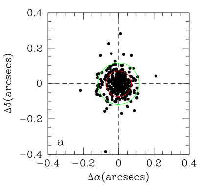
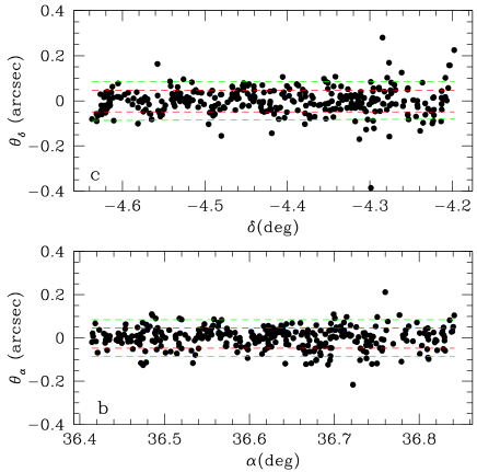
Figure 2: Radial (a), right-ascension (b), and declination (c) residuals between the $K$-band and $i^{\prime}$-band positions for unsaturated, point-like sources. The inner (red) and outer (green) dashed circles/lines enclose 68% and 90% of all objects, respectively. The centroid of the distribution of radial residuals is indicated by crossed dashed lines.

2.1.2 Quality of photometry

The quality checks on the image sequences of the target and standard star fields described above, and the comparison of the magnitudes between the deep and the shallow parts of our $K$-band survey already gave an indication of the reliability of our photometry.

The photometric errors as a function of the K magnitude were estimated by use of repeated exposures on the same region of the sky. The source detection was performed with SExtractor and the MAG_AUTO parameter from the output file was adopted as a measure of the total magnitudes. An example is shown in Fig. 3, where two 30 minutes exposures have been used for the comparison. Since both images contribute equally and independently to the measured error $\sigma$ shown in Fig. 3, the uncertainty for an individual 30 minutes exposure is given by $\sigma/\sqrt{2}$. Then, coadding the two images to obtain the final stacked image (we recall that the typical exposure time for the stacked image is 1 hour) reduces the individual errors by a further factor $1/\sqrt{2}$. Hence, the final error will be a half of the value measured with the above comparison. Therefore, for the final stacked image of a pointing the estimated 1$\sigma$ errors are 0.04, 0.12, and 0.17 mag at $K_{\rm{Vega}}$ = 18,19, and 20 mag, respectively.

As an independent check of the goodness of our photometry, we compared our K-band magnitudes with those from the UKIDSS Early Data Release (Dye et al. 2006) in F02 (Deep Extragalactis Survey, DXS, see figure 14 of Dye et al. (2006) for an indication of coverage and depth) and found them to be in reasonable agreement, although with some spread. No significant systematic offset is present. In Fig. 4 we show the comparison for all cross-identified bona-fide point-like sources that were selected for having a SExtractor FLUX_RADIUS parameter $r_{1/2}\,>\,2.7$ in the $i^{\prime}$-band (see Ilbert et al. 2006) and have $K_{\rm{Vega}}\,<20$ in our catalogue, roughly corresponding to a $>\,10\sigma$ detection on our $K$-band image.

Figure 3: Photometric error as a function of the $K$-band magnitude obtained as comparison of the magnitudes from two 30 min exposures of the same field. The thick solid line indicates the mean magnitude difference between the two images and the thin solid lines indicate the 1$\sigma$ error as a function of the $K_{\rm{Vega}}$ magnitude. The typical 1$\sigma$ error in the magnitudes of the final stacked 1hr exposure will be a half of the error reported in this plot.

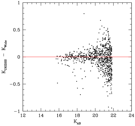
Figure 4: Comparison of our photometry with the $K$-band photometry from the early data release of the UKIDSS survey (Dye et al. 2006). Only point-like sources with a 10$\sigma$ detection were considered. The solid line indicates the mean value of the magnitude difference.

3 The $K$-band catalogue

3.1 Building the catalogue

The construction of the catalogue went through a series of steps aimed at obtaining a catalogue as complete as possible in the $K$-band – suited to the extraction of $K$-selected galaxy samples – while minimising the incidence of spurious detections without affecting our completeness. This goal was achieved by matching the results of two detection procedures, one performed directly on the $K$-band image, and the other based on the use of a $\chi^{2}$ image, constructed using the technique outlined in Szalay et al. (1999). The latter had the main purpose of pruning spurious detections from the catalogue, especially in the $K$-faint regime, and to obtain $K$-band magnitudes already matched with the optical ones, which were obtained starting from the same $\chi^{2}$ detection image (see also McCracken et al. 2003; Radovich et al. 2004, for the use of $\chi^{2}$ images in the preparation of VVDS photometric catalogues in other wavelengths).

The steps we followed are detailed below. The detection and measurement of the sources on the final mosaicked image with the associated weight map were obtained with SExtractor by applying similar criteria to those described in Iovino et al. (2005). As a measure of total magnitudes in our catalogue we use the SExtractor parameter MAG_AUTO.

Step 1. A $\chi^{2}-g^{\prime}r^{\prime}i^{\prime}$ image built from CFHTLS data has been used as the detection image for the measurement of the $K$-band sources with SExtractor in double-image mode. The use of the $\chi^{2}$ image has the advantage of reducing the number of spurious detections, while still picking up most reliable sources that are present in our $K$-band image. The $\chi^{2}$ image and the $K$-wide image have sufficiently similar seeing to assure the effectiveness of this procedure. For an object to be included in our catalogue, it must contain at least three contiguous pixels above a per-pixel detection threshold of 0.4$\sigma$ in the $\chi^{2}$ image. This step produced the version 1 (V1) of our catalogue and offered us a direct cross-identification of the $K$-band sources with those listed in the CFHTLS catalogue for the same region of the sky (Ilbert et al. 2006). The total number

Step 2. A second version of the catalogue (V2) was produced by using SExtractor in single-image mode (i.e. without a separated detection image) on the $K$-wide image. This was a key step for the creation of a $K$-selected catalogue and was necessary to ensure that we would not miss any real $K$-band source that escaped detection on the $\chi^{2}$ image. In this case, to reduce the number of fake detections, we chose to include in the catalogue the objects containing at least 9 contiguous pixels above a per-pixel detection threshold of 1.1$\sigma$.

Step 3. A positional match of sources between the two catalogues was obtained by adopting 1$\aas@@fstack{\prime\prime}$0 as an upper limit to the separation for a source to be considered the same. Tests with different upper limits to the source separation showed that our choice was conservative enough to include all sources present in both catalogues and sufficiently small to minimize false matches. This procedure provided us with a list of objects that were detected in the K-wide image but were not in the $\chi^{2}$ image. Besides truly red objects, this list included members of (apparent) pairs that are resolved in the $K$-band image but appear as an individual source in the $\chi^{2}$ image (see Step 6 below), sources that fall in the vicinity of bright objects and are, therefore, masked by bright halos in the $\chi^{2}$ image, and, finally, a number of fake detections that needed to be expunged.

Step 4. In order to refine the object list produced at Step 3, we evaluated the level of contamination from fake detections as a function of magnitude. To this purpose we applied SExtractor to the inverse of the $K$-wide image, with the same parameters we used for the production of the catalogue V2. The contamination level within 0.5 magnitude bins was estimated as the fraction of detections in the inverse image with respect to the original image. The resulting contamination rate is 9% in the bin centered at $K_{\rm{Vega}}$ = 19.75 and reaches 23% in the bin centered at $K_{\rm{Vega}}$ = 20 (i.e. in the range 19.75 - 20.25 mag). We note that this contamination rate is relevant for the sources that were detected using only the $K$-band image, while it is not representative of the contamination from spurious detections of catalogue V1, for which the effect is minimized by the use of the $\chi^{2}$ image (as demonstrated in Iovino et al. 2005).

To limit the amount of contamination, out of all $K$-band detections for which it was not possible to identify a counterpart in the catalogue V1 we selected those with a magnitude K_Vega $\leq$ 20.25 and, out of these, we retained only the sources that appeared reliable upon visual inspection of the $K$-band and optical images. These remaining 726 sources were added to the catalogue V1. Their magnitudes in the other available bands were determined by running SExtractor on the relevant optical images by using the $K$-band as the detection image.

Step 5. A positional match of our $K$-band detections (catalogue V2) with catalogued VVDS sources in the relevant region of the sky, allowed us to ensure the inclusion in our catalogue of all objects with a measured spectroscopic redshift. At this step we added to our catalogue further 66 K-detected sources. These sources did not have a counterpart in the catalogue V1 because of their vicinity to bright stars in the $\chi^{2}$ image. Also, they were missed by our Step 4 because most of them are fainter than the threshold $K_{\rm{Vega}}$ = 20.25 we adopted for the inclusion of additional sources from the catalogue V2. In fact they are $\ga$ 3$\sigma$ detections with an average magnitude $K_{\rm{Vega}}\,\sim$ 20.9, 13 of them having $K_{\rm{Vega}}\,<$ 20.5.

Step 6. A comparison of the magnitudes of the sources in common between the catalogues V1 and V2 showed a general good agreement, thus indicating that the additional sources identified in catalogue V2 could be safely added to the main catalogue without need of aperture corrections. However, a number of sources showed a remarkable magnitude difference between the two catalogues and required further investigation. We adopted as a criterion to select sources with deviant magnitudes the simultaneous satisfaction of the conditions: $|K_{\rm{Vega\_V1}}\,-\,K_{\rm{Vega\_V2}}|\,>\,5\sigma$ (where $\sigma$ was obtained by adding in quadrature the errors on the individual magnitudes) and $|K_{\rm{Vega\_V1}}\,-\,K_{\rm{Vega\_V2}}|\,>\,0.2$ (to exclude the cases with small absolute deviations but with very small magnitude errors, that would be selected by our first condition). The search was limited to objects brighter than $K_{\rm{Vega}}$ = 20.25, in analogy to Step 4.

About 300 objects were selected this way and visually inspected to check for correct cross-identification between the two catalogues and for the presence of possible problems. These objects were found to include false matches, matches with $K$-band false detections, source blends that had been correctly deblended only in the $K$-band image but not in the $\chi^{2}$ image, and vice-versa, source blends that had been correctly deblended in the $\chi^{2}$-image but remained unresolved as an individual source in the $K$-band image. We corrected the catalogue for the relevant cases, by rejecting false detections and adopting magnitude measurements based on the $K$-band image instead of the $\chi^{2}$-image for blends that were unresolved in the latter. Vice-versa, for blends that were unresolved in the $K$-band but correctly resolved in the $\chi^{2}$-image we kept the identifications and magnitudes of catalogue V1. In both cases the fact that these sources were actually blends of multiple sources and not multiple clumps within a single galaxy appeared obvious from the visual inspection of the individual optical and near-infrared images.

Step 7. For the deep area of the survey, a comparison between the magnitudes obtained using the new $\chi^{2}$ image and those presented in Iovino et al. (2005), based on a $\chi^{2}-BVRIK$ image, did not reveal any systematic difference and showed that the new measurements are equivalent (within the errors) to the original ones. Therefore, for consistency with the previously published paper, in our final catalogue we adopted the original magnitudes for the deep part of the survey.

Step 8. A correction for Galactic extinction on an object-by-object basis was applied to the magnitudes in the final catalogue by using Schlegel et al. (1998) dust maps.

3.2 Completeness

An indicative estimate of the limiting magnitude of our survey can be simply obtained based on the background rms of the coadded images and on the seeing during the observations. The $n\sigma$ magnitude limits are given by mag($n\sigma$) = $zp\,-\,2.5\log(n\sigma\sqrt{A})$, where $zp$ is the zero point and $A$ is the area of an aperture whose radius is the average FWHM of unsaturated point-like sources (see Table 1). The values estimated this way for $n$ = 3, 5 are mag(3$\sigma$) $\sim$ 21.4 and mag(5$\sigma$) $\sim$ 20.9 (in the Vega system). Indeed, by measuring the signal-to-noise ratio as a function of K-band magnitude across the final K-wide image in a 3$\aas@@fstack{\prime}$1-wide running box with a step of 37″(i.e. 200 pixels) (and by imposing the relevant positional constraints to keep the box within the borders of the $K$-wide image as marked with a solid line in Fig. 1) we obtained a magnitude limit for 3$\sigma$ detections that varies in the range $K_{\rm{Vega}}$ = 21.4 - 22.8, the brightest limit being referred to the shallower part of the image, which is the subject of the present paper.

However, a better characterisation of the photometric properties of our final image is given by the estimate of the completeness level in the source detection at various magnitudes. We determined the completeness level from our capability to recover artificial point-like sources inserted at random positions in our image. The detection of artificial sources was performed with the same SExtractor parameters adopted for the real sources. The procedure we followed does not differ from that adopted by Iovino et al. (2005) and we refer the reader to that paper for further details. A representation of the completeness level as a function of magnitude for the shallow part of our $K$-band survey is shown in Fig. 5. In particular we reach a nominal completeness level of 90% (50%) for point-like sources with $K_{\rm{Vega}}$ $\leq$ 20.5 (21.5). The completeness level for the deep part of the survey (as estimated in Iovino et al. 2005) is 90% (50%) to $K_{\rm{Vega}}$ $\leq$ 20.75 (22.00).

However, the determination of the actual completeness of our final catalogue is more complex than described above. In fact, while the completeness test was run on the $K$-band image alone, the use of the $\chi^{2}$-image played a role in the completeness level that was finally achieved. On the other hand, having used the $\chi^{2}$-image for the detection of sources, there is the concern that our catalogue is not a purely K-selected one, at least for the shallow part of the survey that is the object of this paper. As explained in the previous section, for $K_{\rm{Vega}}\,\leq$ 20.25 all sources with a significant detection in the $K$-band image have been included. Furthermore, for $K_{\rm{Vega}}\,\leq$ 20.50 the depth of the images composing the $\chi^{2}$-image implies that the last is fully sufficient to recover sources even with the reddest colors while, at the same time, reducing the number of spurious detections. Therefore, our conclusion is that down to $K_{\rm{Vega}}\,=$ 20.5, where we reach a nominal completeness level of 90% for point-like sources, we can safely state that our catalogue is a truly K-selected one. The achieved completeness level is supported by the raw number counts (see Sect. 6) that do not fall below a power law at least up to $K_{\rm{Vega}}\,=$ 20.5.

Remaining potential problems for the $K_{\rm{Vega}}\,>$ 20.5 regime are i) possible cases of association of $\chi^{2}$-detected sources with correlated noise in the $K$-band image and ii) some possible level of color incompleteness that could arise from missing extremely red, $K$-faint sources that could have remained undetected in the $\chi^{2}$ image. Therefore, for such faint magnitudes regime we cannot state that our catalog is a purely $K$-selected one, having nevertheless been designed to be as complete as possible in both the optical and in K-band. This caveat should be kept in mind when in the next sections we refer to our catalogue as a $K$-selected one: this attribute is, strictly speaking, correct only for $K_{\rm{Vega}}\,<$ 20.5.

Figure 5: Completeness level of our K-shallow survey as a function of magnitude; 50% and 90% completeness levels are marked with dashed lines.

3.3 The $K$-wide photometric sample

Our final $K$-wide catalogue totals 51959 detections. It contains 22846 objects down to our limiting magnitude (i.e. 50% completeness limit) $K_{\rm{Vega}}\,\leq 21.5$ and 10615 objects down to our 90% completeness limit $K_{\rm{Vega}}\,\leq$ 20.5.

However, to be sure to be dealing with a truly K-selected catalogue and to avoid contamination by spurious sources, for future analysis we restrict our final photometric sample to the 8856 objects down to $K_{\rm{Vega}}\,\leq$ 20.25. The number of catalogued objects for different magnitude limits are reported in Table 2 for ease of comparison with other existing surveys. At this level, no distinction has been made between stars and galaxies. This issue is addressed later on, in Sect. 5. The magnitude distribution of the sample is shown in Fig. 6. The photometric redshifts for this sample, determined including the $K$-band information, are presented in Sect. 4.

Table 2: Field F02: $K$-selected photometric sample

$K$$\leq$ 19.0	$K\leq$ 19.5	$K\leq$ 19.75	$K\leq$ 20.0	$K\leq$ 20.25	$K\leq$ 20.5
3608	5152	6180	6399	8857	10615

Figure 6: Magnitude distribution of our $K$-wide photometric sample down to the magnitude limit of the survey $K_{\rm{Vega}}\,\leq$ 21.5 for all objects (yellow filled histogram) and for objects classified as galaxies (red histogram; Sect. 5). The inset shows the $K$-magnitude distribution for the whole $K$-selected spectroscopic sample (yellow filled histogram), for the objects classified as galaxies within it (red histogram; Sect. 5), and for the galaxy subsample with 17.5 $\leq\,I_{\rm{AB}}\,\leq$ 24.0 (dotted blue histogram).

3.4 The $K$-selected spectroscopic sample

Our shallow $K$-band survey and part of the deep one (i.e. all pointings in Fig. 1 except for n1, n2, and n3) are located in the four-pass area of the VVDS, wich implies a spectroscopic sampling rate up to $\sim$ 40% down to $I_{\rm AB}\,\leq$ 24 (Le Févre et al. 2005). Our $K$-wide catalogue (down to the magnitude limit of the survey, intended as the 50% completeness limit) contains a total of 4059 objects covered by spectroscopic observations, out of which 3815 have a successful measure of redshift (81 of them are secondary objects with $I_{\rm{AB}}\,>$ 24). The actual spectroscopic sampling rate for the $K$-wide catalogue down to its 90% completeness limit is 26.6% (27.9% to $K_{\rm{Vega}}\,\leq$ 20.25), while the success rate is $\sim$ 95.5% down to the same magnitude limit. Secure (flags 2, 3, and 4 Le Févre et al. 2005) spectroscopic redshifts are available for 1792 galaxies and 23 active galactic nuclei (AGN) down to $K_{\rm{Vega}}\,\leq$ 20.25 (12 of these objects have $I_{\rm{AB}}\,>$ 24). The number of galaxies and stars in the sample within various magnitude limits and for various levels of spectral quality is summarised in Table 3. The star-galaxy separation for the spectroscopic sample relies on the spectral classification.

Table 3: Field F02: Number of galaxies/stars in the $K$-selected spectroscopic sample

Flags	K$\leq$ 19.0	K $\leq$ 19.5	K$\leq$ 19.75	K$\leq$ 19.8	K$\leq$20.0	K$\leq$20.25	K$\leq$20.5	K$\leq$21.5
any	893 / 176	1303 / 201	1566 / 219	1613 / 222	1810 / 239	2113 / 250	2426 / 265	3489 / 325
1, 21	71 / 7	126 / 11	167 / 12	173 / 12	199 / 14	251 / 14	312 / 15	534 / 27
2, 22	183/ 11	304 /13	385 / 14	394 / 15	456 / 20	551 / 23	656 / 27	1022 / 52
3,4,23,24	613 /158	834/ 177	968/193	999/ 195	1097 / 205	1241 / 213	1375 / 223	1791 / 246
9,29	7/ 0	13/ 0	18/ 0	18/ 0	25 / 0	36 / 0	48 / 0	105/
11, 211, 12, 212	0 / 0	0 /0	0 / 0	0 / 0	3 / 0	3 / 0	2 / 0	2 / 0
13, 14, 213, 214	16 / 0	21 / 0	22 / 0	22 / 0	22/ 0	23 / 0	25 / 0	26 / 0
19, 219	3 / 0	5 / 0	6 / 0	7 / 0	7 / 0	8 / 0	8 / 0	9 / 0

The normalized redshift distribution of our $K$-selected spectroscopic sample down to the magnitude limits $K_{\rm{Vega}}$ $\leq$ 20.25, 20.50 is shown in Fig. 7 in comparison with the redshift distribution of the whole VVDS sample within the same region of the sky. The distribution is presented both for the case of secure redshifts and for all measured redshifts. We distinguish the case in which all available redshifts are considered, irrespective of the $I$-band magnitudes and the case where only objects within the magnitude limits of the spectroscopic survey ($17.5\,\leq\,I_{\rm{AB}}\,\leq\,24.0$) are taken into account. The median redshifts of the distributions down to $K_{\rm{Vega}}$ $\leq$ 20.5 closely approach those of the whole VVDS samples both for secure and less secure redshifts (see values quoted in Fig. 7).

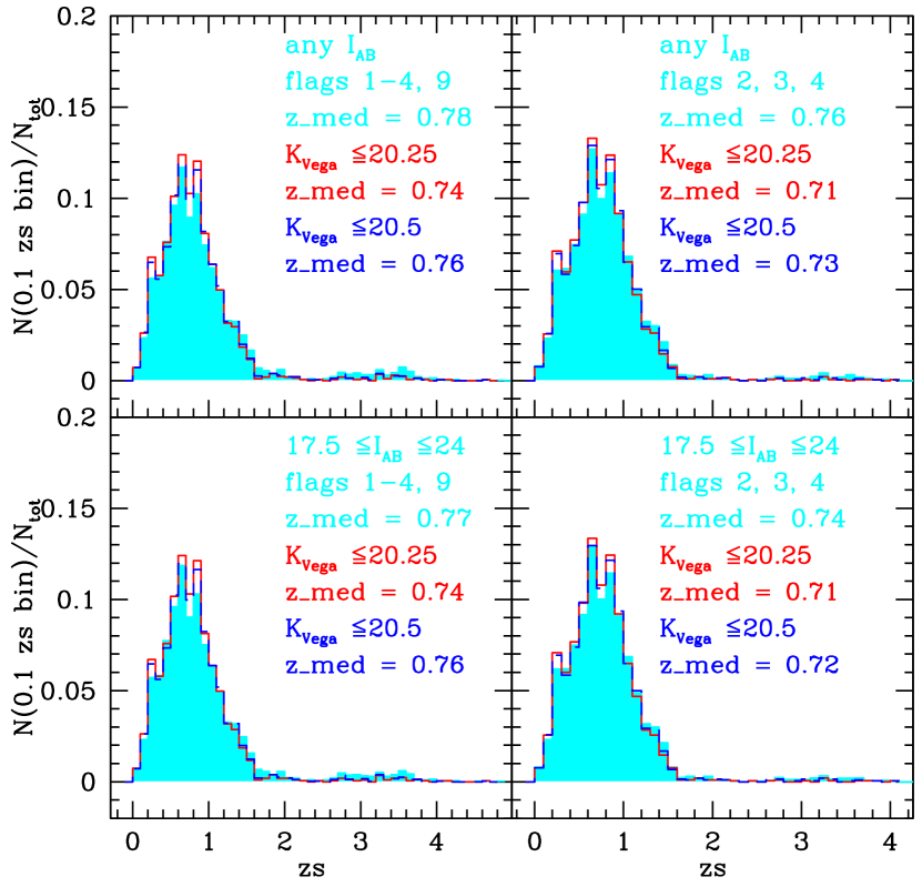
Figure 7: Normalized redshift distribution of the $K$-selected spectroscopic sample (including only sources spectroscopically classified as galaxies) down to $K_{\rm{Vega}}\,\leq$ 20.25 (red empty histogram) and to $K_{\rm{Vega}}\,\leq$ 20.5 (dashed blue line) compared to the one of the entire VVDS sample within the same sky area (cyan filled histogram). The left-hand panels include flags 1-4,9, and their equivalents, whereas the right-hand panels include only secure redshifts with flags 2, 3, 4, 9 and their equivalents. The top panels show the redshift distribution irrespective of the $I$-magnitude values (i.e. including secondary objects falling outside the selection criteria of the spectroscopic survey), whereas the bottom panels show only the objects within the VVDS magnitude selection limits. The median redshifts $z_{med}$ of the distributions are quoted.

The $K$-magnitude distribution of the spectroscopic sample is shown in Fig. 6. The distributions for both the pure $K$-selection and the combined $K$/$I_{\rm{AB}}$-selection are displayed.

A slight incompleteness in colour is present at faint $K$-band magnitudes to the completeness limit of our survey because of the $I_{\rm AB}\,\leq\,24$ magnitude limit of the VVDS specroscopic survey, that tends to disfavour faint red objects. The effect of the spectroscopic $I_{\rm AB}$ magnitude limit is illustrated in Fig. 8, where it is shown that for $K_{\rm{Vega}}\,>$ 19.0 the spectroscopic survey starts missing some objects with red $I-K$ colours. Objects with $I_{\rm AB}\,>\,24$ represent an increasing fraction of progressively bluer sources for increasingly faint $K$ magnitudes. As a result, a $\sim$ 10% (13%) colour incompleteness arises in the 0.5 magnitude bin centered at $K_{\rm{Vega}}$ = 19.75 (20.25). However, photometric redshifts can be used to circumvent this problem.

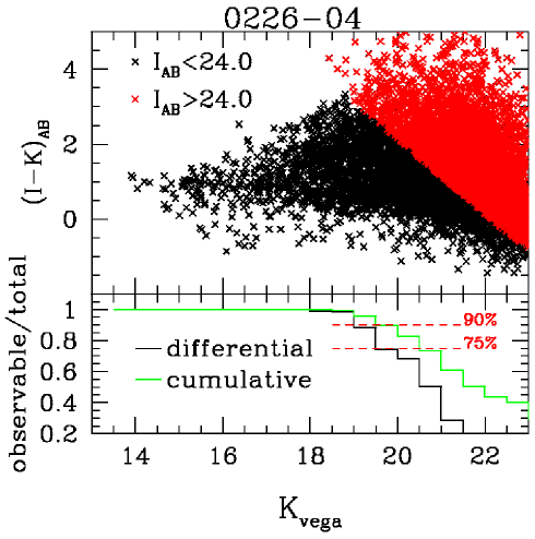
Figure 8: The $I-K$ vs $K$ magnitude diagram for sources with $I_{\rm AB}\,<\,24$ (black) and $I_{\rm AB}\,>\,24$ (red) and the differential (black) and cumulative (green) distributions of $K$ magnitudes illustrate the effects of the $I_{\rm AB}$ magnitude cut of the spectroscopic survey on the completeness of the $K$-selected spectroscopic sample. A slight colour incompleteness arises in the last two 0.5 mag bins down to $K_{\rm{Vega}}\,\leq\,$ 20.5.

4 Photometric redshifts

The photometric redshifts for our $K$-selected sources were obtained with the code Le_Phare (developed by S. Arnouts and O. Ilbert), by following the procedure described in Ilbert et al. (2006) and using MAG_AUTO magnitudes measured in the maximum number of available photometric bands in the set $u^{\ast}g^{\prime}r^{\prime}i^{\prime}z^{\prime}BVRIJK$. $J$-band magnitudes (or upper limits) are available only for a sub-area of $\sim$ 160 arcmin², i.e. for 26% of the objects in our $K$-band catalogue. In all our photometric redshift determinations we applied the corrections for systematic offsets of the zero-points and the optimised galaxy templates described in detail in Ilbert et al. (2006).

As it has been shown by Ilbert et al. (2006), a Bayesian approach (Benítez 2000) with the introduction of an a priori information on the redshift probability distribution function improves significantly the determination of photometric redshifts with respect to the traditional $\chi^{2}$ method. In this work, consistently with Ilbert et al. (2006) and supported by the similarity shown in Fig. 7 between $K\,<$ 20.5 and VVDS redshift distributions, we use directly a prior based on the second one and we compare the results obtained with/without the application of this prior to those obtained with/without the use of the $K$-band photometry in addition to the other bands during the fitting procedure with Le_Phare. This exercise allows us to determine the influence of the $K$-band on the quality of the photometric redshifts. In comparing the photometric redshifts ($zp$) with the spectroscopic ones ($zs$), we express the redshift accuracy in terms of $\sigma_{\Delta z/(1+zs)}$ using the normalised median absolute deviation defined as 1.48 $\times$ median$(|\Delta z|/(1+zs))$, while for the catastrophic errors we adopt the definition $|zs\,-\,zp|/(1+zs)\,>\,0.15$. In analogy to Ilbert et al. (2006), we splitted our $K$-selected spectroscopic sample into an $i^{\prime}$-bright ($17.5\leq i^{\prime}\leq 22.5$) and an $i^{\prime}$-faint ($22.5<i^{\prime}\leq 24.0$) subsample to check the quality of the photometric redshifts. Also, we did our test down to three different limits in $K$ magnitude ($K_{\rm{Vega}}\,\leq$ 20.25, 20.5, 21.5), to evaluate the effects of the inclusion of $K$-faint sources. To ensure the use of reliable photometric redshifts, we considered only those based on $\geq$ 5 photometric bands (including the $K$ band). Moreover, to avoid side-effects related to the quality of spectroscopic redshifts, we limited the comparison to galaxies with spectroscopic flags 3, 4, 23, and 24, although we recognize that this choice could bias our subsamples toward classes of objects whose spectral properties favour the redshift measurement. The results are summarized in Table 4, where we report the values of $\sigma_{\Delta z/(1+zs)}$ and $\eta$ for the selected subsamples of galaxies and the total number of objects we used for our test.

Figure 9 illustrates the effects of the inclusion of the $K$-band and of the prior on the quality of photometric redshifts for the $K$-selected spectroscopic sample down to $K_{\rm{Vega}}\,\leq\,20.25$ (the results for the samples down to fainter $K$ magnitude limits are alike). It is evident that the inclusion of the $K$-band, even without the use of any prior, is more effective than the use of the prior alone in reducing the number of catastrophic redshifts, especially for objects that are erroneously assigned a photometric redshift in the range 2 $<\,zp\,\leq$ 3.5. The best result is obtained with the use of both the $K$-band and the prior, which gives $\sigma_{\Delta z/(1+zs)}$ = 0.026 and $\eta$ = 1.61% for the $i^{\prime}$-bright subsample, and $\sigma_{\Delta z/(1+zs)}$ = 0.028 and $\eta$ = 2.43% for the entire sample, at least in the covered redshift range.

Objects spectroscopically classified as active galactic nuclei are not considered in the comparison shown here. Their inclusion would increment the catastrophic errors, but would leave unchanged the outcome of the comparison, with the best quality of photometric redshifts being achieved by including both the $K$-band and the prior in the fitting process.

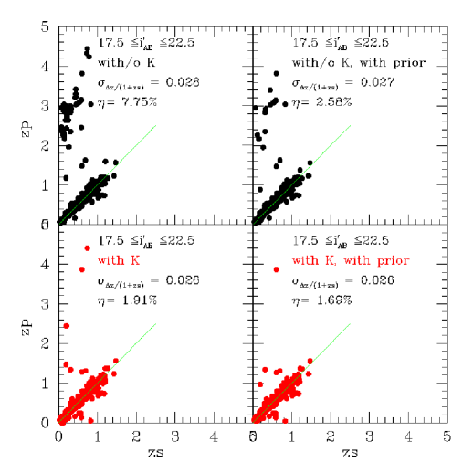
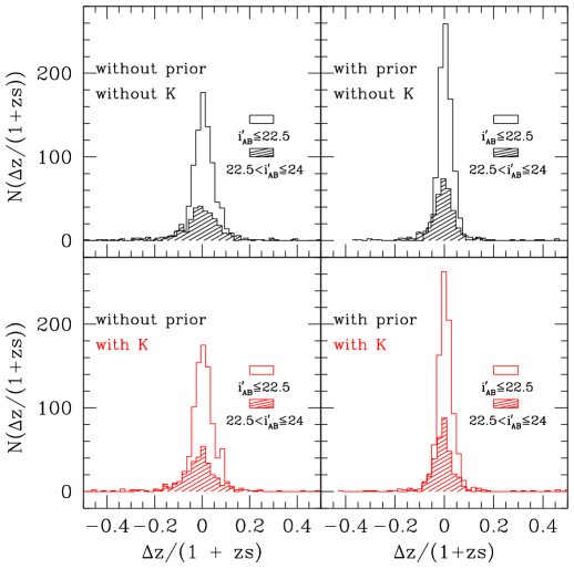
Figure 9: Comparison between spectroscopic and photometric redshifts for the $i^{\prime}$-bright subsample (left-hand panels) and distribution of $\Delta z/(1+zs)$ for the $i^{\prime}$-bright and $i^{\prime}$-faint subsamples (right-hand panels, empty and shaded histograms, respectively). See text for details. The $zp$ = $zs$ line is displayed in green. The results for Le_Phare fits with/without prior and with/without inclusion of $K$-band photometry are shown with the relevant values of $\sigma_{\Delta z/(1+zs)}$ and $\eta$. The results for the fits with the $K$-band are displayed in red.

Table 4: Quality of photometric redshifts determined with/without $K$-band photometry and with/without prior down to different $K$ magnitude limits and for two intervals of $i^{\prime}$ magnitudes. For the comparison we used galaxies with good quality spectroscopic redshifts (flags 3, 4, 23, 24) and with photometric redshifts derived from at least 5 photometric bands, including the $K$ band.

	$K\leq 20.25$	$K\leq 20.5$	$K\leq 21.5$	$K\leq 20.25$	$K\leq 20.5$	$K\leq 21.5$
Nobj	890	917	946	347	453	817
	$17.5\leq i^{\prime}\leq 22.5$			$22.5<i^{\prime}\leq 24.0$
	without $K$, without prior
$\sigma_{\Delta z/(1+z)}$	0.0280	0.0280	0.0280	0.0384	0.0379	0.0351
$\eta$ (%)	7.75	8.18	8.35	7.78	7.73	7.71
	with $K$, without prior
$\sigma_{\Delta z/(1+z)}$	0.0265	0.0265	0.0267	0.0349	0.0345	0.0327
$\eta$ (%)	1.91	1.96	2.11	5.76	5.30	5.38
	without $K$, with prior
$\sigma_{\Delta z/(1+z)}$	0.0270	0.0268	0.0268	0.0381	0.0367	0.0339
$\eta$ (%)	2.58	2.62	2.85	6.05	5.52	5.88
	with $K$, with prior
$\sigma_{\Delta z/(1+z)}$	0.0264	0.0264	0.0265	0.0350	0.0336	0.0322
$\eta$ (%)	1.69	1.75	1.90	4.32	3.97	4.65

Because of the $I_{\rm{AB}}\,\leq\,24$ magnitude limit of the sample upon which the prior is based, we decided to adopt photometric redshifts determined without the prior for sources fainter than this limit. In Fig. 10 we show the photometric redshift distribution of our sample, after the exclusion of candidate stars, identified as described in Sect. 5. The redshift distribution is shown for the two magnitude limits $K_{\rm{Vega}}\,\leq 20.25$ and $K_{\rm{Vega}}\,\leq 20.5$ for a purely $K$-selected sample and for a sample with an additional $I$-selection that reproduces the magnitude limits of the VVDS spectroscopic survey. The effect of the additional $I$-selection is the loss of objects especially at intermediate to high redshift and, therefore, a lowering of the median redshift of the sample. The median redshift of the purely $K$-selected photometric sample down to $K_{\rm{Vega}}\,\leq 20.25\,(20.5)$ is $zp_{med}$ = 0.87 (0.91).

The photometric redshifts determined in this work are used in a companion paper that is dedicated to $K$-selected extremely red objects (Temporin et al. 2008) extracted from our $K$-band wide catalogue.

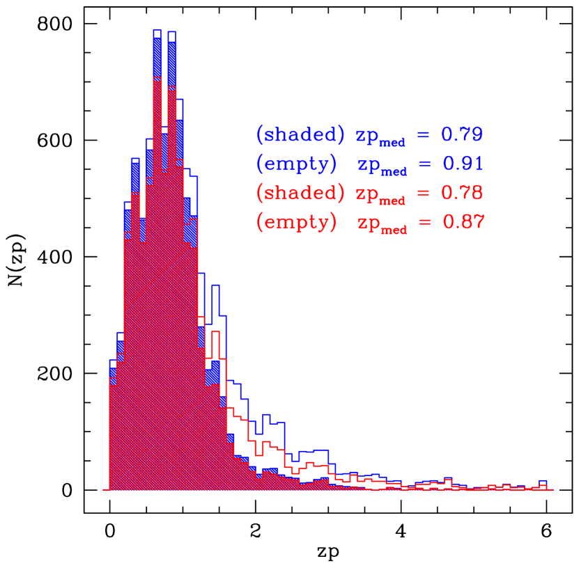
Figure 10: Distribution of photometric redshifts for the $K$-selected photometric samples down to $K_{\rm{Vega}}\,\leq 20.25$ (red) and $K_{\rm{Vega}}\,\leq 20.5$ (blue). Shaded histograms show the redshift distribution when an additional $I$-selection matching the VVDS selection for the spectroscopic survey is applied. The median photometric redshifts of each distribution are reported.

5 Star-galaxy separation

We classified point-like objects with a combination of photometric and morphological criteria, using parameters derived by SExtractor and Le_Phare. We adopted a quite complex strategy since our aim is to perform the star/galaxy separation even at faint magnitudes, where most of the single criteria are known to fail.

The chosen parameters and adopted criteria are the following:

• the CLASS_STAR parameter given by SExtractor, providing the “stellarity-index” for each object; selected point-like sources are obeying CLASS_STAR $\geq 0.95,0.90$ for objects brighter/fainter then $i^{\prime}_{\rm AB}<22.5$ respectively;

• the FLUX_RADIUS parameter, also computed by SExstractor in the $K$-band and denoted as $r_{1/2}$, measuring the radius that encloses $50$% of the object total flux; we imposed $r_{1/2}<3.4$ pixels as the criterion to be satisfied by stellar sources;

• the MU_MAX parameter by SExtractor, representing the peak surface brightness above the background; the locus of selection of stellar objects in the $i^{\prime}$ vs MU_MAX plot has been derived empirically using the spectroscopic sample;

• the $BzK$ criterion, proposed by Daddi et al. (2004), with stars characterized by colours $z-K<0.3(B-z)-0.5$;

• the $\chi^{2}$ and of the SED fitting carried out with Le_Phare during the photometric redshift estimate, by using template SEDs of both stars ($\chi^{2}_{star}$)and galaxies ($\chi^{2}_{gal}$); the criterion to be satisfied by a stellar source is $\chi^{2}_{gal}\,-\,\chi^{2}_{star}\,>$ 0.

The application of the above criteria to the spectroscopic sample is shown in Fig. 11. Objects fulfilling at least 4 of the above mentioned criteria have been classified as point-like, whereas a less restrictive constraint has been imposed for objects brighter than $K_{\rm{Vega}}\,=\,17.16$, with only 3 over 5 criteria fulfilled. Moreover, to be sure not to miss stellar saturated objects, we included to the point-like objects selection all the sources with $r_{1/2}<4$ and $K_{\rm{Vega}}\,<\,14.16$ disregarding the other criteria.

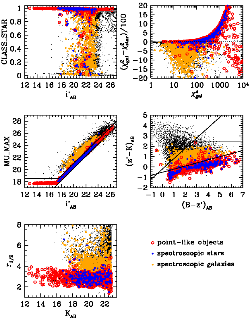
Figure 11: The five criteria for the star-galaxy separation (see text) applied to the spectroscopic sample. From top to bottom, and left to right, the SExtractor CLASS_STAR, MU_MAX, and FLUX_RADIUS parameters, the Le_Phare best-fit $\chi^{2}$ values, and the $BzK$ diagram (Daddi et al. 2004) are plotted. Each panel illustrates an individual photometric criterion and the corresponding candidate stellar sources (red circles), overplotted to spectroscopically classified galaxies (yellow dots) and stars (blue dots).

The selection yields 745 point-like objects at $K_{\rm{Vega}}\,\leq\,20.5$, with 235 of them belonging to the spectroscopic sample. Within this subsample, 80% of the spectroscopic stars are correctly identified and only 3 spectroscopic galaxies and 4 active galactic nuclei with very reliable redshift (flag= 3, 4, 13, 14) fall into the star candidate subsample. The galaxy sample is found to be contaminated by misclassified stars at the 2% level.

This method for the star-galaxy separation represents an improvement over both the method used by Ilbert et al. (2006) and the one adopted by Pozzetti et al. (2007), as we verified on the spectroscopic sample.

Our final classification of the objects takes into account the spectroscopic information when this is flagged as highly reliable (flag = 3, 4, 23, 24, 13, 14, 213, 214) by overriding the photometric classification with the spectroscopic one.

6 Galaxy and star number counts

Comparing number counts of galaxies and stars with published compilations is a good check both of the star-galaxy separation efficiency and of the reliability of our photometry, as well as the sample reliability and completeness. The differential number counts of stars (number 0.5 mag^-1 deg^-2) for the F02 wide field are shown in Figure 12. To avoid underestimating bright-star counts, for this exercise we used the catalogues before excising the areas around bright stars. The continuous line is the prediction of the model of Robin et al. (2003) computed at the appropriate galactic latitude. The agreement between observed and predicted star counts is very good (the error bars shown are Poissonian error bars), confirming the reliability both of our photometry and of our star-galaxy separation procedure.

Figure 13 shows the differential number counts (number (0.5 mag)^-1 deg^-2) for the F02 wide field. The dotted line is obtained by normalising the observed raw number counts to the total field after excising areas around bright stars (616 arcmin²). The error bars shown are Poissonian error bars and no correction for stellar contamination has been applied to the raw counts shown. The contamination estimated from the prediction of the model of Robin et al. (2003) is below 3% for the fainter bins shown in the plot. The heavy continuous line shows the total galaxy counts obtained after correcting the counts for stellar contamination estimated using our star-galaxy separation. We did not apply any further completeness or contamination correction to our data because down to the limiting magnitude ($K_{\rm{Vega}}\,=$ 20.5) plotted in Figure 13 such corrections are negligible.

Figure 12: Differential number counts of stars in the F02 wide field. The continuous lines are the prediction of the model of Robin et al. (2003).

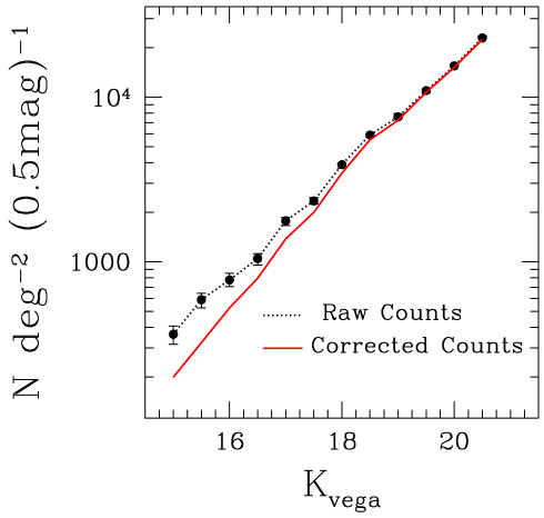
Figure 13: Differential $K-$band number counts in the F02 wide field. The dotted line shows the raw number densities and error bars are Poissonian. The heavy line shows galaxy densities obtained after correcting for star contamination.

Table 5 lists our raw differential counts, the total raw number densities (in units of number (0.5 mag)^-1 deg^-2), and the final, corrected for stellar contamination, galaxy densities together with their $1\sigma$ error bars.

Table 5: Column 2 shows the raw differential number counts per half magnitude bin. Column 3 shows our raw total number densities (number 0.5mag^-1 deg^-2). Column 4 shows our total, differential galaxy densities, corrected for star contamination and Column 5 is their poissonian $1\sigma$ error bar.

$K_{\rm{vega}}$	total	Nraw	Ncorr	$\sigma$
	counts	$0.5\leavevmode\nobreak\$mag${}^{-1}\rm{deg}^{-2}$	$0.5\leavevmode\nobreak\$mag${}^{-1}\rm{deg}^{-2}$
15	62	363	199	34
15.5	100	585	322	43
16	133	778	520	55
16.5	178	1041	801	68
17	302	1766	1374	90
17.5	402	2351	2006	108
18	660	3859	3462	142
18.5	1007	5889	5514	180
19	1309	7655	7275	206
19.5	1881	10999	10614	249
20	2671	15619	15157	298

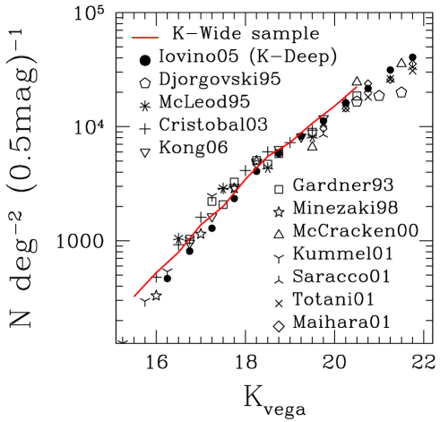
Figure 14: The $K-$band galaxy number counts, in units of number 0.5mag^-1 deg^-2, obtained in this paper are compared to a compilation of those from the literature, including counts from Gardner et al. (1993), Djorgovski et al. (1995), McLeod et al. (1995), Minezaki et al. (1998), McCracken et al. (2000), Kümmel & Wagner (2001), Saracco et al. (2001), Totani et al. (2001), Maihara et al. (2001), Cristóbal-Hornillos et al. (2003), Iovino et al. (2005), and Kong et al. (2006).

Figure 14 show our total corrected galaxy counts (solid line) compared with a selection of literature data. We have followed the approach of Cristóbal-Hornillos et al. (2003) and select only reliable counts data from the literature, considering only data with negligible incompleteness correction and with star-galaxy separation applied. We have been conservative in the selection of the magnitude intervals plotted in our counts, restricting ourselves to bins with relatively large numbers of galaxies, negligible incompleteness and small contamination corrections. The agreement with literature data is very good. Our F02 wide galaxy counts confirm the change of slope around $K_{\rm{Vega}}\,\sim\,18.0$ previously detected by Iovino et al. (2005), Gardner et al. (1993) and Cristóbal-Hornillos et al. (2003). In the range $18\,<\,K_{\rm{Vega}}\,<\,20.5$ the slope of the galaxy counts is $\gamma_{K}\,\sim\,0.30\pm 0.09$, while in the brighter magnitude range, $15.0<K_{\rm{Vega}}<18.0$, the slope is steeper: $\gamma_{K}\,\sim\,0.42\pm 0.02$.

7 Clustering analysis for $K-$selected data

In this Section we investigate the clustering properties of point like and extended sources in the F02 wide $K-$band catalogues.

We use the projected two-point angular correlation function, $\omega(\theta)$, which measures the excess of pairs separated by an angle $\theta,\theta+\delta\theta$ with respect to a random distribution. This statistic is useful for our purposes because it is particularly sensitive to any residual variations of the magnitude zero-point across our stacked images. We measure $\omega(\theta)$ using the standard Landy & Szalay (1993) estimator, i.e.,

$$\omega_{e}(\theta)={\mbox{DD}-2\mbox{DR}+\mbox{RR}\over\mbox{RR}}$$ (1)

with the DD, DR and RR terms referring to the number of data-data, data-random and random-random pairs between $\theta$ and $\theta+\delta\theta$. We use logarithmically spaced bins, with $\Delta log(\theta)=0.2$, and the angles are expressed in degrees, unless stated otherwise. DR and RR are obtained by populating the two-dimensional coordinate space corresponding to the different fields number of random points equal to the number of data points, a process repeated 1000 times to obtain stable mean values of these two quantities.

7.1 Clustering of point-like sources

We first measure the angular correlation function $\omega(\theta)$ of the stellar sources. As stars are unclustered, we expect that, if our magnitude zero-points and detection thresholds are uniform over our field, then $\omega(\theta)$ should be zero at all angular scales.

The results for F02 wide-field $K-$band data are displayed in Figure 15, where the correlation function is plotted for the total sample of stars obtained from our wide field according to the procedure described in section 5: 617 stars in the $K-$band interval $15.00\,\leq\,K\,\leq\,20.25$. At all scales displayed the measured correlation values are consistent with zero. Error bars are obtained through bootstrap resampling of the star sample (and are roughly twice poissonian error bars).

Figure 15: Plot of the correlation function $\omega(\theta)$ for the total sample of stars in the $K-$band stacks as a function of the logarithm of the angular pair separation in degrees. At all scales displayed the measured correlation values are consistent with zero.

7.2 Clustering of extended sources

The procedure followed to measure $\omega(\theta)$ is similar to the one described above for the star sample. In the case of galaxies a positive amplitude of $\omega(\theta)$ is expected, and we have to take into account the so called “integral constraint” bias. If the real $\omega(\theta)$ is assumed to be of the form $A_{\omega}\theta^{\delta}$, our estimator (1) will be offset negatively from the true $\omega(\theta)$, according to the formula:

$$\omega_{e}(\theta)=A_{\omega}(\theta^{-\delta}-C)$$ (2)

This bias increases as the area of observation decreases, and it is caused by the need to use the observed sample itself to estimate its mean density, see eg Peebles (1980). The negative offset AC can be estimated by doubly integrating the assumed true $\omega(\theta)$ over the field area $\Omega$:

$$A_{\omega}C={1\over\Omega^{2}}\int\int\omega(\theta)d\Omega_{1}d\Omega_{2}$$ (3)

This integral can be solved numerically using randomly distributed points for each field:

$$C={\sum N_{rr}(\theta)\leavevmode\nobreak\ \theta^{-\delta}\over\sum N_{rr}(\theta)}$$ (4)

Assuming 1″as the pairs minimal scale at which two galaxies can be distinguished as separated objects, and $\delta=0.8$, we obtain the following value: $C_{Wide}=4.50$.

We estimated the amplitude $A_{\omega}$ for a series of $K$ limited galaxy samples by least square fitting $A(\theta^{-0.8}-C)$ to the observed $\omega(\theta)$, weighting each point using bootstrap error bars. Figure 16 shows the results obtained for 6 different $K-$band limiting magnitudes. No correction for stellar contamination is applied (only the objects classified as stars, using the method described in section 5, were excluded from the analysis) and the error bars on the amplitude are those from the fit.

Figure 17 shows the comparison of our results with literature data. The continuous, dotted, and dashed lines show the models of PLE from Roche et al. (1998), with scaling from local galaxy clustering.

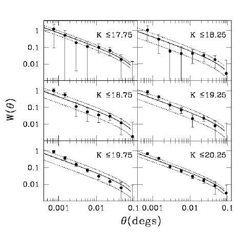
Figure 16: Results obtained for the amplitude $A_{\omega}$ at $1\deg$ of our F02 wide field on galaxy sub-samples of different $K-$band limiting magnitudes. No correction for stellar contamination is applied and the error bars on the amplitude are those obtained from the fit.

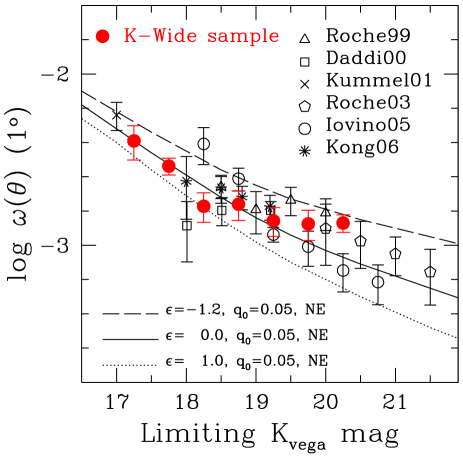
Figure 17: We compare our total sample estimate of the amplitude, $A_{\omega}$ at $1\deg$, of the angular correlation function with a compilation of results from the literature in similar magnitude ranges. We include mesurements from: Roche et al. (1999), Daddi et al. (2000), Kümmel & Wagner (2001), Roche et al. (2003), Iovino et al. (2005), and Kong et al. (2006). The continuous, dotted and dashed lines show, for reference, the models of PLE from Roche et al. (1998), with scaling from local galaxy clustering.

Table 6 lists our amplitude measurements for the F02 sample, in units of $10^{-4}$ at $1\deg$, together with their bootstrap error bars. For each limiting magnitude, the total number of objects N used in the analysis is also listed.

Table 6: Observed $\omega(\theta)$ amplitudes A, in units of $10^{-4}$ at $1\deg$, together with their $1\sigma$ error bars, for our F02 wide field. The number of objects used in the analysis down to the K magnitude faint limits shown in the first column is also listed.

Magnitude	$0226-04$ (F02)
	N	A $\pm$ dA
K $<$ 17.25	561	40.68 $\pm$ 9.24
K $<$ 17.75	902	28.97 $\pm$ 3.25
K $<$ 18.25	1486	16.92 $\pm$ 3.32
K $<$ 18.75	2427	17.39 $\pm$ 3.41
K $<$ 19.25	3661	13.91 $\pm$ 2.67
K $<$ 19.75	5470	13.33 $\pm$ 2.66
K $<$ 20.25	8059	13.49 $\pm$ 1.57

8 Conclusions

We have presented a new $K$-band catalogue that covers a contiguous sky area of 623 arcmin² down to a magnitude limit $K_{Vega}\,\leq\,21.5$ and provides us with a 90% complete $K$-selected sample down to $K_{Vega}\,\leq\,20.5$, although with some possible level of color incompleteness potentially affecting extremely red sources fainter than $K_{Vega}\,=\,20.5$, whose inclusion is disfavoured by the procedure to build the catalogue at these faint magnitudes (see discussion in Sect. 3.2). This is one of the biggest $K$-selected samples available to date to this magnitude limit and is complemented by $UBVRIu^{\ast}g^{\prime}r^{\prime}i^{\prime}z^{\prime}$ photometry – available through the VVDS and CFHTLS surveys – as well as by VVDS spectroscopy with a sampling rate of $\sim$ 27%, down to the 90% completeness limit.

Good quality photometric redshifts have been obtained for the whole sample by following the method outlined by Ilbert et al. (2006) and including the $K$-band photometry in the fits of the galaxy SEDs. By using our spectroscopic subsample we explored the effects of the inclusion of $K$-band photometry in the determination of photometric redshifts. We verified that the use of the $K$ band leads to similar advantages as the training on the spectroscopic redshift distribution function, namely a considerable reduction of the fraction of catastrophic errors. When no a priori spectroscopic information is adopted to train the fitting procedure, the additional use of the $K$ band improves significantly the determination of photometric redshifts, as expected. The results from this survey show that we expect a significant improvement in the accuracy of photometric redshifts obtained by future wide-field surveys using near-infrared data (e.g. the Visible and Infrared Survey Telescope for Astronomy, VISTA).

Also, taking advantage of the $K$-band photometric parameters, we have implemented a quite complex set of criteria for the star-galaxy separation that improved on methods previously adopted by our team (Ilbert et al. 2006; Pozzetti et al. 2007). A very good agreement of star and galaxy number counts with those present in the literature has proven the effectiveness of our star-galaxy separation method as well as the good quality of our photometry and the reliability and completeness of our sample.

The good quality of our photometry as well as the reliability and completeness of the sample are confirmed by the comparison of the number counts of stars and galaxies with published compilations. The $K$-band galaxy number counts from this work are in excellent agreement with those obtained from the $K$-deep sample (Iovino et al. 2005) and with a selection of compilations from the literature. The projected two-point angular correlation function does not show any peculiarity as a function of magnitude and angular scale and is broadly in agreement with results from the literature.

The galaxy mass function, the luminosity function, and the properties of extremely red objects based on our $K$-selected catalogue are presented in companion papers (Pozzetti et al. 2007; Bolzonella et al. 2008; Temporin et al. 2008; Bondi et al. 2008). A cross-match of this $K$-band catalogue with radio sources from the VVDS-VLA deep field has been carried out by Bondi et al. (2007) and has revealed a higher incidence of faint $K$-band counterparts ($K_{\rm{Vega}}\,>\,20$) among candidate ultra-steep-spectrum radio sources with respect to the rest of the radio sources in the sample, although based on small number statistics.