Vibrational resonances in 1D Morse and FPU lattices.

Abstract

In the present paper the resonances of vibrational modes in one-dimensional random Morse lattice are found and analyzed. The resonance energy exchange is observed at some values of elongation. Resonance $2\,\omega_{1}=\omega_{2}$ is investigated in details. The interacting modes are inequivalent: the higher-frequency mode is much more stable in the excited state, i.e. its life-time is larger than the life-time of lower-frequency mode under the resonance conditions. Simple model of two nonlinearly coupled harmonic oscillators is also considered. It allows to get analytical description and to investigate the kinetics and the energy exchange degree vs. such parameters as the resonance detuning and specific energy. The very similar behavior is found in the Morse and the two-oscillatory models, and an excellent agreement between analytical and numerical results is obtained. Analogous resonance phenomena are also found in the random Fermi-Pasta-Ulam lattice under contraction.

PACS numbers: 05.50.+q, 83.10.Rp, 34.50.Ez

Keywords: Morse lattice, FPU lattice, nonlinearity, resonance.

I Introduction

The primary goal of Fermi, Pasta, Ulam and Tsingou (FPUT) FPU55 was to find an energy sharing in one-dimensional lattices with nonlinear interaction between neighboring particles. The authors expected the occurrence of the statistical behavior in a system with coupled nonlinear oscillators due to the nonlinear interaction, leading to the energy equidistribution among the degrees of freedom. Initially, the long-wave vibrations were excited and “Instead of a gradual increase of all the higher modes, the energy is exchanged, essentially, among only a certain few. It is, therefore, very hard to observe the rate of  ”thermalization”  or mixing in our problem, and this was the initial purpose of the calculation.” FPU55 .

Much effort has been undertaken to explain the FPUT results. Two approaches were developed. The first one was to analyze the dynamics of the nonlinear lattice in the continuum limit, which led to the discovery of solitary waves Zab65 . The second approach, advanced by Izrailev and Chirikov, pointed to the overlap of nonlinear resonances Chi60 and an existence of a stochasticity threshold in the FPUT system Izr66 . For strong nonlinearities (or/and large energies) the overlap of nonlinear resonances results in the dynamical chaos which destroys the FPUT recurrence and ensures convergence to thermal equilibrium. (For more details on the FPUT problem see recent reviews devoted to the 50th anniversary of the celebrated paper FPU55 in Focus Issue: The Fermi-Pasta-Ulam Problem — The First Fifty Years, ed. by D.K. Campbell, P. Rosenau, and G.M. Zaslavsky, Chaos 15(1) (2005) ).

In the present paper we thoroughly analyze the resonance between the lowest $(k=1)$ and the next $(k=2)$ vibrational modes previously discovered in the random Morse lattice under the elongation Ast07 . Here we also employ the lattice with the random interaction potential between neighboring particles under different deformation degrees. The lattice randomness makes the vibrational frequencies to be irregular, and the deformation allows to achieve the true resonance conditions. Random FPUT lattice (with random quadratic terms) Liv85 and with alternative masses Zab67 were investigated but no resonances were directly observed.

The model of two nonlinearly coupled harmonic oscillators with the frequencies ratio $\omega_{1}\!:\!\omega_{2}=1\!:\!2$ is also considered. An excellent agreement in dynamics and kinetics of the Morse lattice and the oscillatory model is observed.

The random $\alpha$–FPUT lattice under compression demonstrates the similar behavior as the Morse lattice. The compression of the $\alpha$–FPUT lattice in contrast to the elongation of the Morse lattice is explained by the different signs of cubic terms in an expansion of the Morse potential $(\widetilde{U}_{\text{M}}=x^{2}-x^{3})$ and in the $\alpha$–FPUT lattice $U=x^{2}/2+\alpha x^{3}/3$.

II Resonances in random Morse lattice and two-oscillatory model.

II.1 Random Morse lattice.

We consider the finite–length lattice of $N$ particles interacting via the Morse potential with the rigid boundaries. The potential energy has the form:

$$U_{\text{p}}=\sum_{i=1}^{N+1}\xi_{i}\,U(y_{i});\qquad y_{i}=x_{i}-x_{i-1}\quad(x_{0}=0,\,\,x_{N+1}=L),$$ (1)

where $x_{i}$ is the displacement of $i$th particle from the equilibrium and $U(y)=\left[1-\exp(-y)\right]^{2}$ is the dimensionless Morse potential. $\xi_{i}$ is a random number chosen from the range $[0{.}5-1{.}5]$ and is modeling the random well depth of the interaction potential. The left lattice end is fixed and the right end has an arbitrary coordinate $L>0$. The specific lattice elongation is $\varepsilon=L/(N+1)$.

The true resonance condition ($\sum_{k}m_{k}\omega_{k}=0$; $\{m\}\in\mathbb{Z}$ For61 ), can be achieved at some elongation values (apparently dependent on the set $\left\{\xi_{i}\right\}$ of random values in (1)) as it is demonstrated in Fig. 1. The most long-wave mode ($k=1$) with the energy $E_{0}=10^{-5}$ was initially excited and the energies of vibrational modes under adiabatically slow elongation are shown. Small number of particles $N=10$ and low excitation energy allow to avoid the resonances overlap.

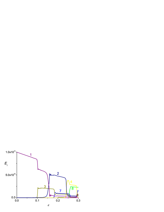
Figure 1: Evolution of the vibrational modes energies vs. the specific elongation $\varepsilon$. The most long-wave mode ($k=1$) is initially excited with the energy $E_{0}=10^{-5}$. Digits numerate the modes numbers. $N=10$. Modes not shown ($k=5,6,9,10$) are not excited.

One can see that the energy exchange is observed at some values of $\varepsilon$. For instance, pair resonances $\omega_{3}\!:\!\omega_{1}=3$ ($\varepsilon\approx 0.101$), $\omega_{2}\!:\!\omega_{1}=2$ ($\varepsilon\approx 0.154$) are obvious. Moreover, triple resonances are also presented (see e.g. $\omega_{3}+\omega_{4}=\omega_{8}$ at $\varepsilon\approx 0.255$). The energy exchange rates and degrees depend on $E_{0}$ and the elongation rate. The energy decrease in Fig. 1 is explained by the “softening” of the potential $U$ in (1) under the elongation Lik06 , i.e. under adiabatic deformations the mode energy $E_{i}$ decreases as its frequency: $E_{i}\sim\omega_{i}$, and $w\sim\sqrt{g}$, where $g$ – lattice rigidity.

The resonance $\omega_{2}\!:\!\omega_{1}=2$ at $\varepsilon\approx 0.154$ is chosen for detailed investigation. But firstly we consider the two-oscillatory model, where the resonance behavior can be analytically described.

II.2 Two-oscillatory model.

We consider two nonlinearly coupled harmonic oscillators with the following hamiltonian (here the main results are briefly demonstrated, whereas the full analysis will be presented elsewhere):

$$H=\dfrac{1}{2}\left(p_{1}^{2}+p_{2}^{2}\right)+\dfrac{1}{2}\left(\kappa_{1}\,q_{1}^{2}+\kappa_{2}\,q_{2}^{2}\right)+\lambda\,q_{1}^{2}\,q_{2}\,,$$ (2)

where $\kappa_{1}=1$, $\kappa_{2}=4$, $\lambda$ is the coupling parameter, and the frequencies ratio is 1:2.

After the variables replacements $q_{i}\mapsto-\sqrt{2\,I_{i}/\omega_{i}}\,\cos\phi_{i}$ and $(2I_{1}-I_{2})/5\mapsto I,\ (2I_{1}-I_{2})/5\mapsto J,\ (2\phi_{1}-\phi_{2})\mapsto\Theta,\ (\phi_{1}+2\phi_{2})\mapsto\Phi$ and the averaging Bog61 ; Arn74 over the period $2\,\pi/\omega_{2}$ Eq. (2) transforms to

$${\widetilde{H}}(I,J)=5\,I-\gamma\,(I+2\,J)\,\sqrt{2\,I-J\,}\,\cos\Theta\,,$$ (3)

where $\gamma=\kappa_{1}\kappa_{2}\,\lambda$. $I$ is the integral of motion and the time evolution is determined by the second term. The energy exchange is governed by the following hamiltonian

$$\mathcal{H}=-\dfrac{{\widetilde{H}}-5\,I}{\gamma\,I}=(1+2\,p)\,\sqrt{2-p}\,\cos\Theta\,,$$ (4)

where $p=J/I$. The initial conditions $p_{0}=2$ and $p_{0}=-1/2$ correspond to the excitation of the oscillators $\omega_{1}=1$ and $\omega_{2}=2$, correspondingly. The Hamiltonian equations for $\mathcal{H}(p,\Theta)$ have the form:

$$\begin{array}[]{lll}\dot{p}&=&(1+2\,p)\,\sqrt{2-p}\,\sin\Theta\,,\vspace{0.3 cm}\\ \dot{\Theta}&=&\dfrac{7-6\,p}{2\,\sqrt{2-p}}\,\cos\Theta\,.\end{array}$$ (5)

1. Excitation of the “stable” oscillator. The initial conditions $p(0)=-1/2,\ \ \Theta(0)=0$ correspond to the excitation of the oscillator $\omega_{2}=2$. In this case the solution of Eq. (5) is

$$\begin{array}[]{rll}p(t)&=&-1/2,\\ \sin\Theta(t)&=&\dfrac{\exp(2\sqrt{10}t)-1}{\exp(2\sqrt{10}t)+1}\end{array}$$ (6)

and $p(t)=$ const, what means that the oscillator $\omega_{2}$ has the infinite life-time and the oscillator $\omega_{1}$ is not excited at all.

2. Excitation of the “unstable” oscillator. The situation drastically changes if the oscillator $\omega_{1}=1$ is initially excited. Since $(p=2,\ \Theta=0)$ is a singular point of (5), the initial condition $p(t=0)=p_{0}=2-\delta$ $(\delta\ll 1)$ should be chosen with the final limiting transition $\delta\to+0$. Taking into account that (5) has the integral of motion $\cos\Theta=\dfrac{(1+2\,p_{0})\,\sqrt{2-p_{0}}}{(1+2\,p)\,\sqrt{2-p}}$ one can get the following solution in the vicinity of $p(t)\sim p_{0}$:

$$p(t)=p_{0}-\dfrac{(12\,p_{0}^{2}-8\,p_{0}-7)}{4}\,t^{2},$$ (7)

and $p(t)$ varies through a finite range in a finite time $\sim\sqrt{4\,\Delta p/a(p_{0})}$ and the phase trajectory goes away from the singular point $p_{0}=2$ over a finite distance. Then, according to (5), $p(t)$ decreases approaching the value $p=-1/2$. It means that the initially excited oscillator $\omega_{1}$ loses its energy in a finite time and completely gives the energy up to the higher frequency oscillator. This allows to specify the oscillator $\omega_{1}$ as an unstable, and the oscillator $\omega_{2}$ as a stable one.

3. “Mixed” initial conditions. Below we briefly consider the “mixed” initial condition $(p_{0}=-1/2+\nu,0)$ when the stable oscillator $\omega_{2}$ is initially excited with small ($\nu\ll 1$) “weight” of the low-frequency oscillator. In this case the energy exchange is also observed and the life-times of both oscillators in excited states can be estimated as:

$$\begin{array}[]{l}\tau_{1}\xrightarrow[p_{0}\to-1/2]{}\dfrac{1}{\sqrt{10}}\,\ln\left(\dfrac{\sqrt{3}+1}{\sqrt{3}-1}\right);\\ \tau_{2}\xrightarrow[p_{0}\to-1/2]{}\dfrac{1}{\sqrt{10}}\,\ln\dfrac{1}{1+2p_{0}}\end{array}$$ (8)

and it follows that if the stable oscillator $\omega_{2}$ is initially excited with a small addition $\nu\ll 1$ of the oscillator $\omega_{1}$, then the energy exchange is observed and the life-time of the unstable lower-frequency oscillator $\tau_{1}$ is finite and does not depend on $\nu$, whereas the life-time $\tau_{2}$ of the stable higher-frequency oscillator increases $\sim-\ln(\nu)$ as $\nu\rightarrow+0$.

4. Resonance detuning. Obviously, the considered exact resonance $\omega_{2}=2\,\omega_{1}$ rarely occurs and the situation of resonance detuning is of particular interest. Let $\kappa_{1}=(1-\mu)$ and $\kappa_{2}=4$ in Eq. (2), where $\mu\ll 1$ means a small resonance detuning. The case of the initial excitation of the stable oscillator is trivial: the equations of motion of (2) are:

$$\ddot{q}_{1}=-(1-\mu)\,q_{1}-2\lambda\,q_{1}q_{2};\qquad\ddot{q}_{2}=-4\,q_{2}-\lambda\,q_{1}^{2}$$ (9)

and if $q_{1}(t=0)=0,\ q_{2}(t=0)\neq 0$ then the first oscillator is not excited at all, and the initially excited second oscillator lives infinitely long independently on the vicinity to the exact resonance.

The case of the initial excitation of the unstable oscillator $\omega_{1}$ requires more accurate analysis. It is convenient to make the variables replacements: $(q_{1}\cos\alpha-q_{2}\sin\alpha)\mapsto y_{1}$ and $(q_{1}\sin\alpha+q_{2}\cos\alpha)\mapsto y_{2}$. Then by neglecting the terms of the order of $\lambda\mu\ll 1$ one can choose $\alpha$ such that the true resonance problem is fulfilled in new variables $\{y_{1},y_{2}\}$. But this problem was considered above. And finally the life-times of both oscillators are estimated as:

$$\begin{array}[]{l}\tau_{1}(\mu)=\dfrac{1}{\sqrt{10}}\,\ln\left(\dfrac{\sqrt{3}+1}{\sqrt{3}-1}\right);\\ \tau_{2}(\mu)=\dfrac{1}{2\sqrt{10}}\,\ln\left(\dfrac{3}{80\,\mu}\right).\end{array}$$ (10)

Thus if the unstable oscillator $\omega_{1}$ is initially excited, then its life-time is a finite value and doesn’t depend on the closeness to the exact resonance point, while the life-time of the stable oscillator increases as $\sim-\ln(\mu)$ at $\mu\to+0$.

Below we numerically compare the kinetics and the energy exchange degree for the Morse lattice and the two-oscillatory model.

III Numerical simulations of resonance interaction in the Morse lattice and two-oscillatory model.

III.1 Comparison of the Morse lattice and two-oscillators model.

Our primary goal is to investigate the rate and the energy exchange degree near the resonance for two most long-wave modes $(k=1,2)$ in the Morse lattice depending on the model parameters (resonance detuning, excitation energy). The comparison is made with the two-oscillatory model and one-to-one correspondence between vibrational modes $k=1,2$ in the Morse lattice and lower and higher frequency oscillators is assumed.

Note, that because of the nonlinearity of both models, the mode/oscillator frequencies depend on the excitation energy $E_{0}$. And the true resonance conditions are fulfilled for some values $\varepsilon_{0}(E_{0})$ and $\mu_{0}(E_{0})\neq 0$. It is convenient to represent the actual values of $\varepsilon$ and $\mu$ as $\varepsilon=\varepsilon_{0}(E_{0})+\varepsilon_{1}$ and $\mu=\mu_{0}(E_{0})+\mu_{1}$, where $\varepsilon_{1}$ and $\mu_{1}$ are the measures of resonances detuning.

We compare the resonance $2\,\omega_{1}=\omega_{2}$ at $\varepsilon\simeq 0{.}154$ (see Fig. 1) in the Morse lattice and the resonance in the two-oscillatory model with $\kappa_{1}=1-\mu$, $\kappa_{2}=4$; parameter $\lambda$ for definiteness is chosen $\lambda=0.3$. The exact resonance values $\mu_{0}$ and $\varepsilon_{0}$ are determined as values, where the largest life-times of the stable mode/oscillator are achieved in numerical simulation. These values are $\varepsilon_{0}(E_{0})=0.153\,808\,281\,3623$ and $\mu_{0}(E_{0})=3{.}374\,961\,52\cdot 10^{-8}$, and $E_{0}=10^{-6}$ in both cases. All digits in $\varepsilon_{0}(E_{0})$ are accurate: variation of the last (13th) digit noticeably diminishes the vibrational life-time.

Thus one can analyze and compare the interaction of vibrational modes and oscillators vs. detuning parameters $\varepsilon_{1}$ and $\mu_{1}$ in both systems.

III.2 Numerical results for the Morse lattice and oscillatory model.

The temporal behavior of modes/oscillators energies is shown in Fig. 2 at different values of detuning parameters $\varepsilon_{1}$ and $\mu_{1}$. Here the unstable mode/oscillator are initially excited with $E_{0}=10^{-6}$.

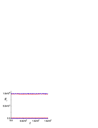
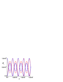
a                                                          b

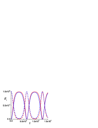
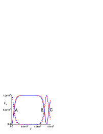
c                                                          d

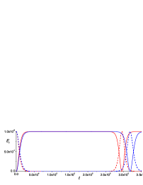
e

Figure 2: Temporal modes/oscillator energies evolution at different values of the resonance detunings for the Morse lattice (blue color) and the two oscillators model (red color). Stable mode/oscillator – solid lines, unstable mode/oscillator – dashed lines. a) $\varepsilon_{1}=-2{.}380\,828\,136\,23\cdot 10^{-2}$, $\mu_{1}=10^{-3}$; b) $\varepsilon_{1}=-8{.}082\,813\,623\cdot 10^{-4}$, $\mu_{1}=4\cdot 10^{-5}$; c) $\varepsilon_{1}=-5{.}828\,136\,23\cdot 10^{-5}$, $\mu_{1}=1{.}9\cdot 10^{-6}$; d) $\varepsilon_{1}=-8{.}136\,23\cdot 10^{-8}$, $\mu_{1}=10^{-9}$; e) $\varepsilon_{1}=0{.}0$, $\mu_{1}=0{.}0$. In all cases the unstable mode/oscillator are initially excited with $E_{0}=10^{-6}$. Note the enlarged time scale in panel e).

The general scenario of the kinetics and the energy exchange degree is very similar for both systems.

There is no interaction between the vibrational modes/oscillators far away from the resonance conditions ($|\varepsilon_{1}|\gtrsim 10^{-2}$ and $|\mu_{1}|\gtrsim 10^{-3}$). There exists partial and symmetrical energy exchange in the middle range of the detuning parameters $10^{-4}\lesssim|\varepsilon_{1}|\lesssim 10^{-2}$ and $10^{-6}\lesssim|\mu_{1}|\lesssim 10^{-3}$ (Figs. 2a-b). As the resonance point is approached (by diminishing $|\varepsilon_{1}|$ and $|\mu_{1}|$) the energy exchange degree and the modes asymmetry increases. And at a certain detuning parameters values the full energy exchange is achieved (Fig. 2c). Further approaching to the resonance point results in the increase of the stable mode/oscillator life-times, whereas the life-times of the unstable mode/oscillator do not change (Figs. 2d-e). And finally the life-times of the stable mode/oscillator achieve their maximal values at the resonance point $|\varepsilon_{1}|=|\mu_{1}|=0{.}0$ (Fig. 2e).

The dependence of the stable mode/oscillator life-times vs. values $\varepsilon_{1}$/$\mu_{1}$ is also the same for both models. The dependence is logarithmic (see Fig. 3a), as predicted by (10). We also found that the unstable oscillator life-time $\tau_{1}$ with very good accuracy varies as $\tau_{1}\sim 1/\lambda$ in a wide range $(10^{-2}\leq\lambda\leq 10^{2})$, where $\lambda$ is the coupling parameter in (2). The mode/oscillator life-times are defined as a time intervals for full energy exchange. For example, $\tau_{2}$ is a time interval between points A and B in Fig. 2d. Similarly $\tau_{1}$ is a time interval between points B and C in Fig. 2d.

Fig. 3b demonstrates the energy exchange degree $\Delta E/E_{0}$ vs. $\varepsilon_{1}$/$\mu_{1}$ for both models in the middle range of the resonance detuning parameters ($10^{-4}\lesssim|\varepsilon_{1}|\lesssim 10^{-2}$ and $10^{-6}\lesssim|\mu_{1}|\lesssim 10^{-3}$). One can see the extreme sensitivity of life-times and energy exchange degree to the variations of detuning parameters.

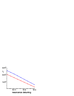
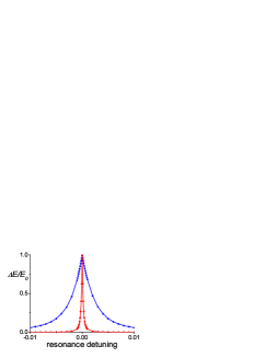
a                                                      b

Figure 3: (a) The dependence of the stable mode/oscillator life-times $\tau_{2}$ on the detuning parameter values for the Morse lattice and the oscillatory model in the vicinity of the exact resonance point; (b) the energy exchange degree vs. the detuning parameter for the Morse lattice and the oscillatory model. The unstable mode/oscillator are initially excited with $E_{0}=10^{-6}$. Blue color – Morse lattice, red color – oscillatory model in both panels.

As pointed above, the exact values for the onset of resonances depend on the excitation energy $E_{0}$. Hence the energy exchange kinetics should be also sensitive to $E_{0}$. Fig. 4 shows the dependencies of the life-times of both modes in the Morse lattice and both oscillators vs. the energy of initially excited unstable mode/oscillator $E_{0}$. The extreme sensitivity of stable mode/oscillatory life-times in the vicinity of exact resonance ($\varepsilon_{0}=0{.}153\,808\,281\,3623$ and $\mu_{0}=3{.}374\,961\,52\cdot 10^{-8}$ at $E_{0}=10^{-6}$) is observed.

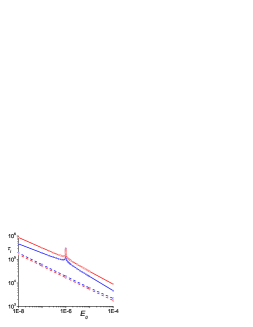
Figure 4: The dependence of modes/oscillators life-times $\tau_{i}$ on the energy of the initially excited unstable mode/oscillator $E_{0}$. Values $\varepsilon_{0}=0{.}153\,808\,281\,3623$ and $\mu_{0}=3{.}374\,96152\cdot 10^{-8}$ correspond to the exact resonance point at $E_{0}=10^{-6}$ ($\varepsilon_{1}=\mu_{1}=0{.}0$). Morse lattice – blue color, oscillatory model – red color; solid lines – stable mode/oscillator, dashed lines – unstable mode/oscillator.

Thus, in the case of the initial excitation of unstable mode/oscillator the resonance behavior is the same in both models and is perfectly described by the analytical results in Sec. II.2. But the models have different features in the case of stable mode/oscillator initial excitation. In the oscillatory model the initially excited stable oscillator lives infinitely long independently on the closeness to the resonance point. The stable mode in the Morse lattice has finite life-time and the energy exchange is observed, the resonance behavior being independent on the resonance detuning. This different features of the models is caused by the addition terms in the Morse potential expansion which influence the energy exchange. Actually, an addition of the term ${\widetilde{\lambda}}\,q_{1}\,q_{2}^{2}$ in (2) results in the mode energy exchange and the finite life-time of the stable vibrational mode.

The case of “mixed” initial conditions when the stable mode/oscillator is excited with a small addition of the unstable mode/oscillator is also analyzed and results are in good agreement with analytical predictions (see (10) ). Fig. 5 shows the dependence of the stable mode/oscillator life-times vs. the contribution of the unstable mode/oscillator energy into the total initial energy $E_{0}$. Here the initial energies of the stable and unstable modes/oscillators are $(1-\nu)E_{0}$ and $\nu E_{0}$, correspondingly.

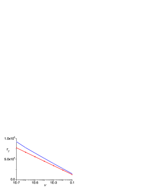
Figure 5: The dependence of the stable mode/oscillator life-times $\tau_{2}$ on the contribution of the unstable mode/oscillator energy $\nu$ into the total initial energy $E_{0}=10^{-6}$. The initial energies of the stable and unstable modes are $(1-\nu)E_{0}$ and $\nu E_{0}$, correspondingly; $\varepsilon_{1}=\mu_{1}=0{.}0$. Blue color – $\tau_{2}$ for the Morse lattice, red color – $\tau_{2}$ for the oscillatory model.

Note that the observed resonance interaction of the vibrational modes is the general phenomenon in random lattices under the deformations at low temperatures. Actually an expansions of any interaction potentials have the form ${\widetilde{U}}\sim x^{2}\pm\gamma\,x^{3}$. The minus sign means that the potential softens under elongation (as in the Morse lattice). On contrary the plus sign (as in the $\alpha$-FPUT lattice) means that the potential softens under contraction. This is the reason which allowed to observe the similar resonance behavior in the random FPUT lattice under contraction.

IV Conclusions.

In conclusion, we briefly summarize the main results.

1. The vibrational modes resonance was found in the random Morse lattice. Two features allow to observe the resonances: the lattice randomness (random values of the interaction potential; the random masses also can be used), and the lattice deformation. At some values of the specific elongation the exact resonance condition $\sum m_{i}\,\omega_{i}=0$ are be fulfilled. The resonance $2\omega_{1}=\omega_{2}$ of two most long-wave vibrational modes was chosen for the detailed analysis. Small number of particles ($N=10$) and low excitation energy allowed to avoid the resonances overlap.

2. Simple two-oscillators model with inharmonic coupling was also considered. The analytical description of the kinetics and modes energy exchange vs. the model parameters (resonance detuning, specific energy) was performed.

3. Surprisingly good agreement was observed for the kinetics and energy exchange rate for the Morse lattice and simple model of two nonlinear coupled harmonic oscillators.

4. Modes/oscillatory life-times and the energy exchange degree are extremely sensitive to the resonance detuning parameters.

5. The resonance behavior is a general feature of random nonlinear lattices at deformations and it was also observed in the random $\alpha$-FPUT lattice.

The observed resonance phenomenon can not throw some light on the problem of energy equipartition and onset of the chaos because of small values of $N$ and low specific energy, but it can serve as a starting point for the analysis of initial stages of vibrational modes interaction.

This work was supported by the RFBR Grant # 08–02–00253.

References

- (1) E. Fermi, J. Pasta, and S. Ulam in Collected Papers of Enrico Fermi, ed. E. Segre, Vol. II (University of Chicago Press, 1965) p.978.
- (2) N. J. Zabusky and M. D. Kruskal, Phys. Rev. Lett. 15, 240 (1965).
- (3) B. V. Chirikov, J. Nucl. Energy Part C: Plasma Phys. Accel. Thermonucl. 1, 253 (1960).
- (4) F. M. Izrailev and B. V. Chirikov, Sov. Phys. Dokl. 11, 30 (1966).
- (5) T. Yu. Astakhova, V. N. Likhachev, and G. A. Vinogradov, Phys. Lett. A 371, 475 (2007).
- (6) R. Livi, M. Pettini, S. Ruffo, M. Sparpaglione, and A. Vulpiani, Phys. Rev. A 31, 1039 (1985).
- (7) N. J. Zabusky and G. S. Deem, Journ. Comp. Phys. 2, 126 (1967).
- (8) J. Ford, J. Math. Phys. 2, 387 (1961).
- (9) V. N. Likhachev, T. Yu. Astakhova, and G. A.Vinogradov, Phys. Lett. A 354, 264 (2006).
- (10) N. N. Bogoliubov and Y. A. Mitropolsky, Asymptotic Methods in the Theory of Nonlinear Oscillations (Gordon and Breach, New York, 1961).
- (11) V. I. Arnol’d, Mathematical Methods. Averaging Method in Classical Mechanics ( Nauka, Moscow, 1974) [in Russian].
- (12) Th. Dauxois, arXiv:0801.1590v1 [physics.hist-ph].