Long Range Electromagnetic Effects involving Neutral Systems and Effective Field Theory

We analyze the electromagnetic scattering of massive particles with and without spin wherein one particle (or both) is electrically neutral. Using the techniques of effective field theory, we isolate the leading long distance effects, both classical and quantum mechanical. For spinless systems results are identical to those obtained earlier via more elaborate dispersive methods. However, we also find new results if either or both particles carry spin.

1 Introduction

There has been a good deal of recent interest in higher order corrections to electromagnetic scattering. In particular the one-photon-exchange approximation, which has traditionally been used to analyze electron scattering has been shown to be inadequate when applied to the problem of isolating nucleon form factors via Rosenbluth separation—inclusion of two-photon-exchange contributions has been found to be essential in resolving small discrepancies with the values of these same form factors as obtained from spin correlation measurements[1]. A second arena where two-photon-exchange effects are needed is the in the analysis of transverse polarization asymmetry measurements in electron scattering. Such quantities vanish in the one-photon-exchange approximation meaning that the sizable effects found experimentally must arise from two-photon effects[2].

Much has been written about such higher order photon processes and a number of groups have undertaken precision calculation of such effects[3]. It is not our purpose here to attempt such detailed calculations of charged particle interactions or to confront experimental data. Rather our goal is to use the methods of effective field theory (EFT) in order to analyze the very longest range (smallest momentum transfer) contributions to the electromagnetic scattering process when one or both of the scattering particles are neutral. These long range components are associated with pieces of the scattering amplitude which are nonanalytic (and singular) in the momentum transfer. Some of these corrections are classical ($\hbar$-independent) and behave as $1/\sqrt{-q^{2}},\sqrt{-q^{2}},etc.$ while others are quantum mechanical ($\hbar$-dependent) and behave as $\log-q^{2},q^{2}\log-q^{2},etc.$, where $q^{2}$ is the momentum transfer[5]. In the case of two spinless charged particles the lowest order interaction, which arises from one-photon exchange, is the simple Coulomb interaction, which behaves as $\alpha/r$, where $\alpha=e^{2}/4\pi$ is the fine structure constant. The contribution to this charged scattering process from two-photon exchange is a problem addressed nearly two decades ago by Feinberg and Sucher using dispersive methods[6]. Even earlier Iwasaki had studied the classical piece of this problem using standard noncovariant perturbation theory[7]. Recently we reexamined this problem, using the methods of effective field theory (EFT)[8]. Results for spinless scattering were found to agree with those of [6] and [7], but the use of EFT methods permitted the extraction of new and interesting spin-dependent structure.

Our goal in the present note is to extend these considerations to the case of the electromagnetic scattering of two nonzero mass particles, at least one of which is neutral. In this case there exists no lowest order Coulomb potential and the leading contribution arises from two-photon exchange. The interaction of two spinless systems was considered long ago by Casimir and Polder[9] and by Feinberg and Sucher[10] in the neutral-neutral case and by Bernabeu and Tarrach[13] and by Feinberg and Sucher in the case of the interaction of a neutral and a charged particle[14]. The first of these calculations was performed using noncovariant fourth order perturbation theory, while the latter evaluations were done using dispersive methods. In the present paper we reanalyze these problem using EFT techniques. The basic idea is to calculate the infrared singular components of the two-photon-exchange diagrams, since such terms give rise to the longest order interactions in coordinate space. In the case of spinless scattering, we will reproduce the results of previous authors[10, 14, 13]. However, the use of EFT methods allows the straightforward extraction of the new and interesting structure which arise if either or both particles carry spin.

In the next section we study the interaction of two neutral particles, while in the following chapter we look at the situation when one of these particles is charged. We present a brief summary in a concluding section.

2 Neutral-Neutral Scattering

The electromagnetic interaction of two neutral systems having separation $r$, the so-called Van der Waals force, was considered long ago by London[15], who gave a simple form for the interaction potential in terms of the electric polarizabilities of the two systems—

$$V_{vdW}(r)\sim-{\alpha_{E}^{a}\alpha_{E}^{b}\omega_{0}\over 4\pi r^{6}}$$ (1)

where $\omega_{0}$ is a typical excitation energy. The form of the vanderWaals potential can be understood in terms of the energy of the dipole moment of ”atom” $b$ ($d_{b}=-ex_{b}$) in the electric field created by the dipole moment of ”atom” $a$—

$${\cal H}_{1}\sim-d_{b}E_{b}(d_{a})=ex_{b}\times{-ex_{a}\over 4\pi r^{3}}=-{e^{2}x_{a}x_{b}\over 4\pi r^{3}}$$ (2)

Of course, $<x_{a}>=<x_{b}>=0$, i.e., there exists no average dipole moment, so this energy change vanishes in first order perturbation theory

$${\Delta E}_{1}=<\psi_{0}|{\cal H}_{1}|\psi_{0}>=0.$$

However, there is a shift at second order since at any given instant of time there exists an instantaneous dipole moment in atom $a$ say. The corresponding electric field from atom $a$ at the position of atom $b$—$E_{a}(R)$—generates a correlated electric dipole moment due to its electric polarizability—

$$d_{b}=4\pi\alpha_{E}^{b}E_{a}(R)=4\pi\alpha_{E}^{b}{ex_{a}\over 4\pi r^{3}}$$ (3)

The electric field generated by this electric dipole moment then acts back on the original atom, yielding an energy

$$\Delta E_{vdw}\sim-d_{a}E_{b}(r)=-{e^{2}x_{a}^{2}\alpha_{E}^{b}\over 4\pi r^{6}}$$ (4)

which is the Van der Waals interaction. What makes this work, then, is the point that one can use the instantaneous position of one atom to provide an action at a distance correlation with a second atom in the vicinity. Finally, we note that the electric polarizability itself can be extracted by calculating the shift in energy of the atom in the presence of an external electric field $E_{0}$ in second order perturbation theory

$$\Delta E^{(2)}=\sum_{n\neq 0}{<0|eE_{0}x_{a}|n><n|eE_{0}x_{a}|0>\over E_{0}-E_{n}}\equiv-{1\over 2}4\pi\alpha_{E}^{a}E_{0}^{2}$$ (5)

We find then $\alpha_{E}^{a}\sim e^{2}<x_{1}^{2}>/\omega_{0}$ and

$$\Delta E_{vdw}\sim{\alpha_{E}^{a}\alpha_{E}^{b}\omega_{0}\over 4\pi r^{6}}$$ (6)

so that it is this self-interaction energy which is responsible for the London form.

Casimir and Polder generated a general form for the interaction potential from quantum mechanics by using two-photon exchange and fourth-order noncovariant perturbation theory[9]. Their result reproduces the simple London form at short distance—$r\leq{1\over\omega_{0}}$ but at large distances, when retardation is important, i.e., when a typical quantum mechanical excitation time $T_{qm}\sim 1/\omega_{0}$ is smaller than the time for light to travel between the two particles $T_{\gamma}\sim r$ then the London potential, which depends upon the correlation between the instantaneous positions of the two systems, breaks down and the interaction evolves into the ong distance asymptotic form

$$V_{CasPol}(r)\stackrel{{\scriptstyle R\rightarrow\infty}}{{\longrightarrow}}{-23(\alpha_{E}^{a}\alpha_{E}^{b}+\beta_{M}^{a}\beta_{M}^{b})+7(\alpha_{E}^{a}\beta_{M}^{b}+\alpha_{E}^{b}\beta_{M}^{a})\over 4\pi r^{7}}$$ (7)

That the very long distance asymptotic form must vary as $1/r^{7}$ is clear from simple scaling, as argued by Kaplan[16]. The argument is elementary—since polarizabilities have units of volume, and since the interparticle separation is the only scale in the problem, the form of the potential must be

$$V\sim-{\alpha_{E}^{a}\alpha_{E}^{b}\over r^{7}}.$$

The derivation of the Casimir-Polder form—Eq. 7—within modern quantum field theory was given by Feinberg and Sucher using dispersive methods[10]. In an impressive calculation using simple assumptions involving analyticity they were able to obtain the Casimir-Polder result.

In this section we shall show how the same form can be obtained in a much simpler and more direct fashion using the methods of effective field theory. The basic idea is to calculate the diagram for two-photon exchange between the two systems and then to retain only the leading nonanalytic—small momentum transfer—terms, since it is these pieces which lead to the dominant—large $r$—behavior of the potential. We first set the generic framework for our study. We examine the electromagnetic scattering of two particles—particle $a$ with mass $m_{a}$ and incoming four-momentum $p_{1}$ and particle $b$ with mass $m_{b}$ and incoming four-momentum $p_{3}$. After undergoing scattering the final four-momenta of particle $a$ is $p_{2}=p_{1}-q$ and that of particle $b$ is $p_{4}=p_{3}+q$—cf. Figure 1. Now we need to be more specific.

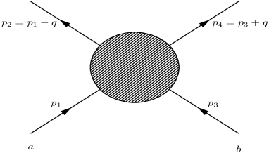
Figure 1: Basic kinematics of electromagnetic scattering.

2.1 Spinless Neutral-Spinless Neutral Scattering

First suppose that the two particles are both neutral and spinless. Then the leading piece of the electromagnetic amplitude is that for two photon emission and can be characterized in terms of the electric and magnetic polarizabilities—$\alpha_{E},\beta_{M}$—which are in turn defined via the energies[11]

$${}^{0}\delta E^{(1)}=-{1\over 2}(4\pi\alpha_{E}\vec{E}^{2}+4\pi\beta_{M}\vec{B}^{2})$$ (8)

For a spinless neutral particle $a$ of mass $m_{a}$ having four-momentum $p_{1}$, the amplitude to emit a photon with polarization $\epsilon_{a}$ and four-momentum $k$ together with a second photon having polarization $\epsilon_{b}$ and four-momentum $q-k$ is then

$$\epsilon_{a}^{*\alpha}\epsilon_{b}^{*\beta}{}^{0}\tau_{\alpha\beta}^{a}(p_{1},k,q-k)$$ (9)

$$= -i4\pi\alpha_{E}^{a}{1\over m_{a}^{2}}(\epsilon_{a}^{*\alpha}k\cdot p_{1}-k^{\alpha}\epsilon_{a}^{*}\cdot p_{1})(\epsilon_{b\alpha}^{*}(q-k)\cdot p_{1}-(q-k)_{\alpha}\epsilon_{b}^{*}\cdot p_{1})$$

$$- i4\pi\beta_{M}^{a}{1\over m_{a}^{2}}(\epsilon^{\alpha\beta\gamma\delta}\epsilon^{*}_{a\beta}k_{\gamma}p_{1\delta})(\epsilon_{\alpha\rho\sigma\lambda}\epsilon^{*\rho}_{b}(q-k)^{\sigma}p_{1}^{\lambda})$$

The two-photon-exchange diagram between spinless neutral particles is shown in Figure 2 and is of the form

$${}^{00}{\cal M}_{2\gamma}(q)$$

$$= {1\over 2!}{(4\pi)^{2}\over m_{a}^{2}m_{b}^{2}}\int{d^{4}k\over(2\pi)^{4}}{-i\eta^{\alpha\gamma}\over k^{2}}{-i\eta^{\beta\delta}\over(k-q)^{2}}{}^{0}\tau^{a}_{\alpha\beta}(p_{1},k,q-k){}^{0}\tau^{b}_{s\gamma\delta}(p_{3},-k,k-q)$$

$$= {1\over 2!}{(4\pi)^{2}\over m_{a}^{2}m_{b}^{2}}\int{d^{4}k\over(2\pi)^{4}}{1\over k^{2}(k-q)^{2}}\left[\alpha_{E}^{b}\left(\eta^{\alpha\beta}p_{3}\cdot kp_{3}\cdot(k-q)+p_{3}^{\alpha}p_{3}^{\beta}k\cdot(k-q)\right.\right.$$

$$- \left.\left.(k-q)^{\alpha}p_{3}^{\beta}p_{3}\cdot k-p_{3}^{\alpha}k^{\beta}p_{3}\cdot(k-q)\right)+\beta_{M}^{b}(\epsilon^{\lambda\alpha\gamma\delta}k_{\gamma}p_{3\delta})({\epsilon_{\lambda}}^{\beta\kappa\mu}(k-q)_{\kappa}p_{3\mu})\right]$$

$$\times \left[\alpha_{E}^{a}\left(\eta^{\alpha\beta}p_{1}\cdot kp_{1}\cdot(k-q)+p_{1\alpha}p_{1\beta}k\cdot(k-q)\right.\right.$$

$$- \left.\left.(k-q)_{\alpha}p_{1\beta}p_{1}\cdot k-p_{1\alpha}k_{\beta}p_{1}\cdot(k-q)\right)+\beta_{M}^{b}({\epsilon^{\lambda}}_{\alpha\sigma\tau}k^{\sigma}p_{1}^{\tau})({\epsilon_{\lambda\beta\kappa\mu}(k-q)^{\kappa}p_{1}^{\mu}})\right]$$

(10)

Figure 2: Bubble diagram used to evaluate the electromagnetic scattering of two neutral systems.

Performing the indicated contractions and integrating, using the results in Appendix A, we find the result

$${}^{00}{\cal M}_{2\gamma}(q)=-{Lq^{4}\over 240}\left[23\left(\alpha_{E}^{a}\alpha_{E}^{b}+\beta_{M}^{a}\beta_{M}^{b}\right)-7\left(\alpha_{E}^{a}\beta_{M}^{b}+\alpha_{E}^{b}\beta_{M}^{a}\right)\right]$$ (11)

where we have defined $L=\log-q^{2}$. In order to determine the potential, we Fourier transform and find, using the results from Appendix B,

$${}^{00}V_{2\gamma}(r)=-\int{d^{3}q\over(2\pi)^{3}}{\cal M}_{2\gamma}(q)e^{-i\vec{q}\cdot\vec{r}}={-23(\alpha_{E}^{a}\alpha_{E}^{b}+\beta_{M}^{a}\beta_{M}^{b})+7(\alpha_{E}^{a}\beta_{M}^{b}+\alpha_{E}^{b}\beta_{M}^{a})\over 4\pi r^{7}}$$ (12)

which is the classic result of Casimir and Polder[9].

2.2 Nonzero Spin Neutral-Spinless Neutral Scattering

If either neutral particle has spin, the potential becomes more complex, but is still straightforward. We must now characterize the system in terms both of its ordinary electric and magnetic polarizabilities but also in terms of so-called ”spin polarizabilities.” If the particle $a$ has spin $S_{a}$, then the leading order spin-dependent generalization of Eq. 8 has the form[12]

$${}^{S_{a}}\delta E_{tot}={}^{0}\delta E^{(1)}<S_{a},m_{af}|S_{a},m_{ai}>+{}^{S_{a}}\delta E^{(2)}$$ (13)

where

$$\delta E^{(2)} = -4\pi\left[\gamma_{E1}^{a}\vec{S}_{a}\cdot\vec{E}\times\dot{\vec{E}}+\gamma_{M1}^{a}\vec{S}_{a}\cdot\vec{B}\times\dot{\vec{B}}\right.$$

$$- \left.2\gamma_{E2}^{a}\left(\vec{E}\cdot\vec{\nabla}\vec{S}_{a}\cdot\vec{B}+E_{j}\vec{S}_{a}\cdot\vec{\nabla}B_{j}\right)+2\gamma_{M2}^{a}\left(\vec{B}\cdot\vec{\nabla}\vec{S}_{a}\cdot\vec{E}+B_{j}\vec{S}_{a}\cdot\vec{\nabla}E_{j}\right)\right]$$

(14)

Here $\vec{S}_{a}=<S_{a},m_{af}|\vec{S}|S_{a},m_{ai}>$ and $\gamma_{E1}^{a},\gamma_{M1}^{a},\gamma_{E2}^{a},\gamma_{M2}^{a}$ are the spin-polarizabilities of the particle. The two-photon vertex of particle $a$ then has the form

$$\epsilon_{a}^{*\alpha}\epsilon_{b}^{*\beta}{}^{S_{a}}\tau_{\alpha\beta}^{a}(p_{1},k,q-k)$$ (15)

$$= {4\pi\over m_{a}^{2}}\left[\alpha_{E}^{a}(\epsilon_{a}^{*\alpha}k\cdot p_{1}-k^{\alpha}\epsilon_{a}^{*}\cdot p_{1})(\epsilon_{b\alpha}^{*}(q-k)\cdot p_{1}-(q-k)_{\alpha}\epsilon_{b}^{*}\cdot p)\right.$$

$$+ \left.\beta_{M}^{a}(\epsilon^{\alpha\beta\gamma\delta}\epsilon_{a\beta}^{*}k_{\gamma}p_{1\delta})(\epsilon_{\alpha\rho\sigma\lambda}\epsilon_{b}^{*\rho}(q-k)^{\sigma}p_{1}^{\lambda})\right]<S_{a},m_{af}|S_{a},m_{ai}>$$

$$+ \gamma_{E1}^{a}i\epsilon_{\alpha\beta\gamma\delta}S_{a}^{\alpha}\left[(\epsilon_{b}^{*\beta}(q-k)\cdot p_{1}-(q-k)^{\beta}\epsilon_{b}^{*}\cdot p_{1})k^{\gamma}(\epsilon_{a}^{*\delta}k\cdot p_{1}-k^{\delta}\epsilon_{a}^{*}\cdot p_{1})\right.$$

$$+ \left.(\epsilon_{a}^{*\beta}k\cdot p_{1}-k^{\beta}\epsilon_{a}^{*}\cdot p_{1})(q-k)^{\gamma}(\epsilon_{b}^{*\delta}(q-k)\cdot p_{1}-(q-k)^{\delta}\epsilon_{b}^{*}\cdot p_{1})\right]$$

$$+ \gamma_{M1}^{a}i\epsilon_{\alpha\beta\gamma\delta}S_{b}^{\alpha}\left[\epsilon^{\beta\rho\lambda\xi}\epsilon_{b}^{*\rho}(q-k)_{\lambda}p_{1\xi}k_{\gamma}\epsilon^{\delta\kappa\zeta\sigma}\epsilon_{a\kappa}^{*}k_{\zeta}p_{1\sigma}\right.$$

$$+ \left.\epsilon^{\beta\kappa\zeta\sigma}\epsilon_{a\kappa}^{*}k_{\zeta}p_{1\sigma}(q-k)^{\gamma}\epsilon^{\delta\rho\lambda\xi}\epsilon_{b}^{*\rho}(q-k)_{\lambda}p_{1\xi}\right]$$

$$+ 2\gamma_{E2}^{a}\left[S_{b}\cdot k(\epsilon_{b}^{*\rho}(q-k)\cdot p_{1}-(q-k)^{\rho}\epsilon_{b}^{*}\cdot p_{1})i\epsilon_{\rho\kappa\zeta\sigma}\epsilon_{a}^{*\kappa}k^{\zeta}p_{1}^{\sigma}\right.$$

$$+ \left.S_{b}\cdot(q-k)(\epsilon_{a}^{*\rho}k\cdot p_{1}-k^{\rho}\epsilon_{a}^{*}\cdot p_{1})i\epsilon_{\rho\kappa\zeta\sigma}\epsilon_{b}^{*\kappa}(q-k)^{\zeta}p_{1}^{\sigma}\right.$$

$$+ \left.(\epsilon_{b}^{*}\cdot k(q-k)\cdot p_{1}-(q-k)\cdot k\epsilon_{b}^{*}\cdot p_{1})i\epsilon_{\rho\kappa\zeta\sigma}S_{a}^{\rho}\epsilon_{a}^{*\kappa}k^{\zeta}p_{1}^{\sigma}\right.$$

$$+ \left.(\epsilon_{a}^{*}\cdot(q-k)k\cdot p_{1}-(q-k)\cdot k\epsilon_{a}^{*}\cdot p_{1})i\epsilon_{\rho\kappa\zeta\sigma}S_{a}^{\rho}\epsilon_{b}^{*\kappa}(q-k)^{\zeta}p_{1}^{\sigma}\right]$$

$$+ 2\gamma_{M2}^{a}\left[S_{a}\cdot k(\epsilon_{a}^{*\rho}k\cdot p_{1}-k^{\rho}\epsilon_{a}^{*}\cdot p_{1})i\epsilon_{\rho\kappa\zeta\sigma}\epsilon_{b}^{*\kappa}(q-k)^{\zeta}p_{1}^{\sigma}\right.$$

$$+ \left.S_{a}\cdot(q-k)(\epsilon_{b}^{*\rho}(q-k)\cdot p_{1}-(q-k)^{\rho}\epsilon_{b}^{*}\cdot p_{1})i\epsilon_{\rho\kappa\zeta\sigma}\epsilon_{a}^{*\kappa}k^{\zeta}p_{1}^{\sigma}\right.$$

$$+ \left.i\epsilon_{\rho\kappa\zeta\sigma}k^{\rho}\epsilon_{b}^{*\kappa}(q-k)^{\zeta}p_{1}^{\sigma}(\epsilon_{a}^{*}\cdot S_{a}k\cdot p_{1}-k\cdot S_{a}\epsilon_{a}^{*}\cdot p_{1})\right.$$

$$+ \left.i\epsilon_{\rho\kappa\zeta\sigma}(q-k)^{\rho}\epsilon_{a}^{*\kappa}k^{\zeta}p_{1}^{\sigma}(\epsilon_{b}^{*}\cdot S_{a}(q-k)\cdot p_{1}-(q-k)\cdot S_{a}\epsilon_{b}^{*}\cdot p_{1})\right]$$

and the scattering amplitude becomes

$${}^{S_{a}0}{\cal M}_{2\gamma}(q)={1\over 2!}{(4\pi)^{2}\over m_{a}^{2}m_{b}^{2}}\int{d^{4}k\over(2\pi)^{4}}{-i\eta^{\alpha\gamma}\over k^{2}}{-i\eta^{\beta\delta}\over(k-q)^{2}}{}^{S_{a}}\tau^{a}_{\alpha\beta}(p_{1},k,q-k){}^{0}\tau^{b}_{s\gamma\delta}(p_{3},-k,k-q)$$ (16)

Performing the various contractions and integration, we find

$${}^{S_{a}0}{\cal M}_{2\gamma}^{tot}(q)={}^{S_{a}0}{\cal M}_{2\gamma}^{a}(q)+{}^{S_{a}0}{\cal M}_{2\gamma}^{b}(q)$$ (17)

with

$${}^{S_{a}0}{\cal M}_{2\gamma}^{a}(q)=-{Lq^{4}\over 240}<S_{a},m_{af}|S_{a},m_{ai}>\left[23\left(\alpha_{E}^{a}\alpha_{E}^{b}+\beta_{M}^{a}\beta_{M}^{b}\right)-7\left(\alpha_{E}^{a}\beta_{M}^{b}+\alpha_{E}^{b}\beta_{M}^{a}\right)\right]$$ (18)

and

$${}^{S_{a}0}{\cal M}_{2\gamma}^{b}(q) = -{Lq^{4}\over 240}{i\over m_{a}^{2}}\epsilon_{\alpha\beta\gamma\delta}p_{1}^{\alpha}p_{3}^{\beta}q^{\gamma}S_{a}^{\delta}\left[4(\alpha_{E}^{b}+\beta_{M}^{b})(\gamma_{E1}^{a}+\gamma_{M1}^{a})\right.$$ (19)

$$+ \left.20(\alpha_{E}^{b}+\beta_{M}^{b})(\gamma_{E2}^{a}+\gamma_{M2}^{a})\right]$$

The first piece here is identical to the form found in the spinless case but is multiplied by the spin-independent factor $<S_{a},m_{af}|S_{a},m_{ai}>=\delta_{m_{af}m_{ai}}$. The second component, however, is spin-dependent and more interesting. Working in the center of mass frame with $\vec{p}_{3}=-\vec{p}_{1}\equiv\vec{p}_{CM}$ and taking the nonrelativistic limit we find

$${}^{S_{a}0}{\cal M}_{2\gamma}^{b}(q) = i{Lq^{4}(m_{a}+m_{b})\over 240m_{a}^{2}}\vec{S}_{a}\cdot\vec{p}_{CM}\times\vec{q}\left[4(\alpha_{E}^{b}+\beta_{M}^{b})(\gamma_{E1}^{a}+\gamma_{M1}^{a})\right.$$

$$+ \left.20(\alpha_{E}^{b}+\beta_{M}^{b})(\gamma_{E2}^{a}+\gamma_{M2}^{a})\right]$$

(20)

Taking the Fourier transform, and noting that $\vec{r}\times\vec{p}_{CM}=\vec{L}$ is the angular momentum, we obtain then

$${}^{S_{a}0}V(r)=-\int{d^{3}q\over(2\pi)^{3}}e^{-i\vec{q}\cdot\vec{r}}{}^{S_{a}0}{\cal M}_{2\gamma}^{tot}(q)$$ (21)

$$= <S_{a},m_{af}|S_{a},m_{ai}>{-23(\alpha_{E}^{a}\alpha_{E}^{b}+\beta_{M}^{a}\beta_{M}^{b})+7(\alpha_{E}^{a}\beta_{M}^{b}+\alpha_{E}^{b}\beta_{M}^{a})\over 4\pi r^{7}}$$

$$+ {m_{a}+m_{b}\over m_{a}^{2}}\vec{S}_{a}\cdot\vec{p}_{CM}\times\vec{\nabla}{1\over\pi r^{7}}\left[(\alpha_{E}^{b}+\beta_{M}^{b})(\gamma_{E1}^{a}+\gamma_{M1}^{a})+5(\alpha_{E}^{b}+\beta_{M}^{b})(\gamma_{E2}^{a}+\gamma_{M2}^{a})\right]$$

$$= <S_{a},m_{af}|S_{a},m_{ai}>{-23(\alpha_{E}^{a}\alpha_{E}^{b}+\beta_{M}^{a}\beta_{M}^{b})+7(\alpha_{E}^{a}\beta_{M}^{b}+\alpha_{E}^{b}\beta_{M}^{a})\over 4\pi r^{7}}$$

$$+ {m_{a}+m_{b}\over m_{a}^{2}}\vec{S}_{a}\cdot\vec{L}{7\over\pi r^{9}}\left[(\alpha_{E}^{b}+\beta_{M}^{b})(\gamma_{E1}^{a}+\gamma_{M1}^{a})+5(\alpha_{E}^{b}+\beta_{M}^{b})(\gamma_{E2}^{a}+\gamma_{M2}^{a})\right]$$

The potential has a spin-independent piece which is simply the Casimir-Polder result, accompanied by a shorter range spin-orbit component, which can be identified by its characteristic spin dependence. Clearly, higher order polarizabilities will lead to new and shorter range interactions as well as spin-spin correlations in the case of scattering of two neutral particles both of which carry spin. However, we will end our discussion here for the neutral-neutral case and move on the situation that one of the particles carries a charge.

3 Spinless Neutral-Charged Particle Interaction

The long range interaction between a neutral and charged system was known classically long before its first quantum mechanical calculation. In this case the presence of a charge $e$ at the origin leads to an electric field at location $\vec{r}$ of size $\vec{E}(\vec{r)}=e\hat{r}/4\pi r^{2}$. If there exists a neutral particle at this location there will be an induced electric dipole moment $\vec{d}_{E}=4\pi\alpha_{E}\vec{E}$. the corresponding interaction energy is

$$\delta E=-{1\over 2}\vec{d}_{E}\cdot\vec{E}(\vec{r})=-{1\over 2}4\pi\alpha_{E}\vec{E}^{2}(\vec{r})=-{\alpha_{E}\alpha\over 2r^{4}}$$

where $\alpha=4\pi e^{2}$ is the fine structure constant.

A full quantum mechanical calculation leads to quantum corrections to this result and was first performed by Bernabeu and Tarrach using dispersive methods[13]. The problem was later reexamined dispersively by Feinberg and Sucher[14]. The result found for the leading long range potential between charged and neutral spinless systems was

$$V(r)=-{1\over 2}{\alpha\alpha_{E}\over r^{4}}+{(11\alpha_{E}+5\beta_{M})\alpha\hbar\over 4\pi mr^{5}}+\ldots$$ (22)

We see that the leading term is classical ($\hbar$-independent) and agrees with the result found in the simple derivation above—$V_{cl}(r)\sim-\alpha\alpha_{E}/r^{4}$. However, there exist additional contributions to the potential which are quantum mechanical in nature and have the form $V_{qm}(r)\sim\alpha\alpha_{E}\hbar/mr^{5}$. Numerically these corrections are tiny. However, such terms are intriguing in that their origin appears to be associated with zitterbewegung. That is, classically we can define the potential by measuring the energy when two objects are separated by distance $r$. However, in the quantum mechanical case the distance between two objects is uncertain by an amount of order the Compton wavelength due to zero point motion—$\delta r\sim\hbar/m$. This leads to the replacement

$$V(r)\sim{1\over r^{4}}\longrightarrow{1\over(r\pm\delta r)^{4}}\sim{1\over r^{4}}\mp 4{\hbar\over mr^{5}}$$

which is the form found in our calculations.

3.1 Spinless Charged–Spinless Neutral Particle

The EFT evaluation of the charge-neutral interaction proceeds similarly to that done for two neutral particles, except that the two photon emission from the charged particle is characterized by the usual vertices—for a spinless charged particle we have the one- and two-photon vertices

$${}^{0}\tau^{(1)}_{\mu}(p_{2},p_{1}) = -ie(p_{1}+p_{2})_{\mu}$$

$${}^{0}\tau^{(2)}_{\mu\nu}(p_{2},p_{1}) = 2ie^{2}\eta_{\mu\nu}$$ (23)

The relevant diagrams are shown in Figure 3 and the associated amplitudes are

$${}^{0}{\cal M}_{2\gamma}^{a}(q) = e^{2}{4\pi\over m_{b}^{2}}\int{d^{4}k\over(2\pi)^{4}}{\eta_{\alpha\gamma}\eta_{\beta\delta}\over k^{2}(k-q)^{2}}\left[\alpha_{E}^{b}\left(\eta^{\alpha\beta}p_{3}\cdot kp_{3}\cdot(k-q)+p_{3}^{\alpha}p_{3}^{\beta}k\cdot(k-q)\right.\right.$$

$$- \left.\left.(k-q)^{\alpha}p_{3}^{\beta}p_{3}\cdot k-p_{3}^{\alpha}k^{\beta}p_{3}\cdot(k-q)\right)+\beta_{M}^{b}(\epsilon^{\lambda\alpha\zeta\sigma}k_{\zeta}p_{3\sigma})(\epsilon^{\lambda\beta\kappa\mu}(k-q)_{\kappa}p_{3\mu})\right]$$

$$\times (2p_{1}-k-q)^{\delta}{1\over(p_{1}-k)^{2}-m_{a}^{2}}(2p_{1}-k)^{\gamma}$$

$${}^{0}{\cal M}_{2\gamma}^{b}(q) = 2e^{2}{1\over 2!}{4\pi\over m_{b}^{2}}\int{d^{4}k\over(2\pi)^{4}}{\eta_{\alpha\beta}\over k^{2}(k-q)^{2}}\left[\alpha_{E}^{b}\left(\eta^{\alpha\beta}p_{3}\cdot kp_{3}\cdot(k-q)+p_{3}^{\alpha}p_{3}^{\beta}k\cdot(k-q)\right.\right.$$

$$- \left.\left.(k-q)^{\alpha}p_{3}^{\beta}p_{3}\cdot k-p_{3}^{\alpha}k^{\beta}p_{3}\cdot(k-q)\right)+\beta_{M}^{b}(\epsilon^{\lambda\alpha\gamma\delta}k_{\gamma}p_{3\delta})({\epsilon_{\lambda}}^{\beta\kappa\mu}(k-q)_{\kappa}p_{3\mu})\right]$$

(24)

Figure 3: Triangle and bubble diagrams used to evaluate the electromagnetic scattering of a charged and a neutral system.

Doing the indicated contractions and performing the integration via the forms given in Appendix A, we find

$${}^{0}{\cal M}_{2\gamma}^{a}(q) = -{\alpha q^{2}\over 4m_{a}}\alpha_{E}^{b}\left(5L+2m_{a}S\right)$$

$${}^{0}{\cal M}_{2\gamma}^{b}(q) = -{\alpha q^{2}\over 12m_{a}}\left(-4\alpha_{E}^{b}+5\beta_{M}^{b}\right)L$$ (25)

where we have defined $S=\pi^{2}/\sqrt{-q^{2}}$. Adding, we find

$${}^{0}{\cal M}_{2\gamma}^{tot}(q)=-{\alpha q^{2}\over 12m_{a}}\left[6m_{a}S\alpha_{E}^{b}+L(11\alpha_{E}^{b}+5\beta_{M}^{b})\right]$$ (26)

whose Fourier transform, using the results given in Appendix B, is

$${}^{0}V(r)=-\int{d^{3}q\over(2\pi)^{3}}{}^{0}{\cal M}_{2\gamma}^{tot}(q)e^{-i\vec{q}\cdot\vec{r}}=-{1\over 2}{\alpha\alpha_{E}^{b}\over r^{4}}+{(11\alpha_{E}^{b}+5\beta_{M}^{b})\alpha\hbar\over 4\pi m_{a}r^{5}}$$ (27)

in complete agreement with Eq. 22. Now consider the modifications which result if spin is introduced.

3.2 Charged Spin 1/2–Spinless Neutral Particle

In order to see what changes result if the charged particle carries spin, suppose particle $a$ has spin 1/2. Then the calculation goes through as before except that we must use the one- and two-photon vertices

$${}^{1\over 2}\tau^{(1)}_{\mu}(p_{2},p_{1}) = -ie\bar{u}(p_{2})\gamma_{\mu}u(p_{1})$$

$${}^{1\over 2}\tau^{(2)}_{\mu\nu}(p_{2},p_{1}) = 0$$ (28)

and we find

$${}^{1\over 2}{\cal M}_{2\gamma}^{a}(q) = -{\alpha q^{2}\over 12m_{a}}\left[\alpha_{E}^{b}\left(\bar{u}(p_{2})u(p_{1})(7L+3Sm_{a})+{1\over m_{b}}\bar{u}(p_{2})\not\!{p}_{3}u(p_{1})(4L+3m_{a}S)\right)\right.$$

$$+ \left.\beta_{M}^{b}\left(\bar{u}(p_{2})u(p_{1})(L-3Sm_{a})+{1\over m_{b}}\bar{u}(p_{2})\not\!{p}_{3}u(p_{1})(4L+3Sm_{a})\right)\right]$$

$${}^{1\over 2}{\cal M}_{2\gamma}^{b}(q) = 0$$ (29)

Using the identity

$$\bar{u}(p_{2})\gamma_{\mu}u(p_{1})=\left({1\over 1-{q^{2}\over 4m_{a}^{2}}}\right)\left[{(p_{1}+p_{2})_{\mu}\over 2m_{a}}\bar{u}(p_{2})u(p_{1})-{i\over m_{a}^{2}}\epsilon_{\mu\beta\gamma\delta}q^{\beta}p_{1}^{\gamma}S_{a}^{\delta}\right]$$ (30)

where

$$S_{a}^{\mu}={1\over 2}\bar{u}(p_{2})\gamma_{5}\gamma^{\mu}u(p_{1})$$

is the spin vector and reduces to

$$S_{a}^{\mu}\stackrel{{\scriptstyle NR}}{{\longrightarrow}}(0,\vec{S}_{a})=\left(0,\chi_{f}^{a\dagger}{1\over 2}\vec{\sigma}\chi_{i}^{a}\right)$$

in the nonrelativistic limit, the full amplitude can be written as

$${}^{1\over 2}{\cal M}_{2\gamma}^{tot}(q) = -{\alpha q^{2}\over 12m_{a}}\left[\bar{u}(p_{2})u(p_{1})\left(\alpha_{E}^{b}(11L+6m_{a}S)+5\beta_{M}^{b}\right)\right.$$ (31)

$$+ \left.{i\over m_{a}^{2}m_{b}}\epsilon_{\alpha\beta\gamma\delta}p_{3}^{\alpha}p_{1}^{\beta}q^{\gamma}S_{a}^{\delta}(4L+3m_{a}S)(\alpha_{E}^{b}+\beta_{M}^{b})\right]$$

Taking the nonrelativisitic limit via

$$\bar{u}(p_{2})u(p_{1})\stackrel{{\scriptstyle\rm NR}}{{\longrightarrow}}\chi_{f}^{a\dagger}\chi_{i}^{a}-{i\over 2m_{a}^{2}}\vec{S}_{a}\cdot\vec{p}_{2}\times\vec{p}_{1}$$ (32)

we find the nonrelativistic amplitude in the center of mass frame

$${}^{1\over 2}{\cal M}_{2\gamma}^{tot}(q) \simeq -{\alpha q^{2}\over 12m_{a}}\left[\left(6m_{a}S\alpha_{E}^{b}+L(11\alpha_{E}^{b}+5\beta_{M}^{b})\right)\chi_{f}^{a\dagger}\chi_{i}^{a}\right.$$ (33)

$$+ \left.{i\over 2m_{a}^{2}}\vec{S}_{a}\cdot\vec{p}_{2}\times\vec{p}_{1}\left(3{m_{a}\over m_{b}}S(m_{a}\alpha_{E}^{b}+(m_{a}+m_{b})\beta_{M}^{b})\right.\right.$$

$$+ \left.\left.{1\over 2m_{b}}L((8m_{a}-3m_{b})\alpha_{E}^{b}+(8m_{a}+3m_{b})\beta_{M}^{b}\right)\right]$$

We observe that the resulting amplitude contains two components—a spin-independent piece whose form is identical to that found in the spinless case accompanied by a new spin-dependent form. Taking the Fourier transform, we find the effective potential

$${}^{1\over 2}V(r) = \int{d^{3}q\over(2\pi)^{3}}{}^{1\over 2}{\cal M}_{2\gamma}^{tot}(q)e^{-i\vec{q}\cdot\vec{r}}=\left(-{1\over 2}{\alpha\alpha_{E}^{b}\over r^{4}}+{(11\alpha_{E}^{b}+5\beta_{M}^{b})\alpha\hbar\over 4\pi m_{a}r^{5}}\right)\chi_{f}^{a\dagger}\chi_{i}^{a}$$ (34)

$$- {1\over 2m_{a}^{2}}\vec{S}_{a}\cdot\vec{p}_{CM}\times\vec{\nabla}\left({\alpha\over 4m_{b}r^{4}}\left(m_{a}\alpha_{E}^{b}+(m_{a}+m_{b})\beta_{M}^{b}\right)\right.$$

$$- \left.{\alpha\hbar\over 8\pi m_{b}m_{b}r^{5}}\left((8m_{a}-3m_{b})\alpha_{E}^{b}+(8m_{a}+3m_{b})\beta_{M}^{b}\right)\right)$$

$$= \left(-{1\over 2}{\alpha\alpha_{E}^{b}\over r^{4}}+{(11\alpha_{E}^{b}+5\beta_{M}^{b})\alpha\hbar\over 4\pi m_{a}r^{5}}\right)\chi_{f}^{a\dagger}\chi_{i}^{a}$$

$$- {1\over 2m_{a}^{2}m_{b}}\vec{S}_{a}\cdot\vec{L}\left({\alpha\over r^{6}}\left(m_{a}\alpha_{E}^{b}+(m_{a}+m_{b})\beta_{M}^{b}\right)\right.$$

$$- \left.{5\hbar\alpha\over 8\pi m_{a}r^{7}}\left((8m_{a}-3m_{b})\alpha_{E}^{b}+(8m_{a}+3m_{b})\beta_{M}^{b}\right)\right)$$

The potential then has a universal spin-independent form accompanied by a spin-orbit component, which in turn will be seen to have a universal structure. In order to verify this assertion, we proceed to the case that particle $a$ has unit spin.

3.3 Charged Spin 1–Spinless Neutral Particle

In order to verify our conjecture that the spin-orbit piece has a universal structure, we perform the scattering calculation for the case of a charged spin 1 particle, which we take to be a $W^{+}$ boson. In order to determine the correct interaction vertices we must recall that the electroweak interaction is a gauge theory. This means that the spin one Lagrangian which contains the charged-W has the Proca form—

$${\cal L}=-{1\over 4}(\vec{U}_{\mu\nu})^{2}+{m^{2}\over 2}\vec{U}_{\mu}^{2}$$ (35)

but the SU(2) field tensor $\vec{U}_{\mu\nu}$ contains an additional term on account of the required gauge invariance

$$\vec{U}_{\mu\nu}=\pi_{\mu}\vec{U}_{\nu}-\pi_{\nu}\vec{U}_{\mu}-ik\vec{U}_{\mu}\times\vec{U}_{\nu}$$ (36)

where $k$ is the SU(2) electroweak coupling constant. This additional term in the field tensor is responsible for the interactions involving three and four W-bosons and for an ”extra” interaction term which has the form of an anomalous magnetic moment and, when added to the simple Proca moment, increases the predicted gyromagnetic ratio from its naive value—$g_{W^{\pm}}^{\rm naive}=1$—to its standard model value—$g_{W^{\pm}}^{\rm sm}=2$[18]. The resulting one- and two-photon vertices are then found to be

$$\tau_{\mu}(p_{2},p_{1}) = -ie\left[(p_{2}+p_{1})_{\mu}\epsilon_{f}^{a*}\cdot\epsilon_{i}^{a}-\epsilon_{f\mu}^{a*}\epsilon_{i}^{a}\cdot p_{2}-\epsilon_{i\mu}^{a}\epsilon_{f}^{a*}\cdot p_{1}\right.$$

$$+ \left.\epsilon_{f\mu}^{a*}\epsilon_{i}^{a}\cdot(p_{1}-p_{2})-\epsilon_{i\mu}^{a}\epsilon_{f}^{a*}\cdot(p_{1}-p_{2})\right]$$

$$\tau_{\mu\nu}(p_{2},p_{1}) = ie^{2}(2g_{\mu\nu}\epsilon_{f}^{a*}\cdot\epsilon_{i}^{a}-\epsilon_{i\mu}^{a}\epsilon_{f\nu}^{a*}-\epsilon_{f\mu}^{a*}\epsilon_{i\nu}^{a})$$ (37)

where we take the incoming spin 1 particle to have polarization vector $\epsilon_{i}^{a}$ satisfying $\epsilon_{i}^{a}\cdot p_{1}=0$ and the outgoing particle to have polarization vector $\epsilon_{f}^{a}$ satisfying $\epsilon_{f}^{a}\cdot p_{2}=0$. Evaluating the diagrams shown in Figure 3 we find then

$${}^{1}{\cal M}_{2\gamma}^{a}(q) = {\alpha q^{2}\over 48m_{a}}\left[\alpha_{E}^{b}\left(2\epsilon_{f}^{a*}\cdot\epsilon_{i}^{a}(29L+12m_{a}S)+{1\over m_{a}^{2}}\epsilon_{f}^{a*}\cdot q\epsilon_{i}^{a}\cdot q(20L+9m_{a}S)\right.\right.$$

$$- \left.\left.{2\over m_{a}m_{b}^{2}}\epsilon_{f}^{a*}\cdot p_{3}\epsilon_{i}^{a}\cdot q(L(m_{a}-8m_{b})-6m_{a}m_{b}S)-{8\over m_{b}^{2}}\epsilon_{f}^{a*}\cdot p_{3}\epsilon_{i}^{a}\cdot p_{3}L\right.\right.$$

$$- \left.\left.{2\over m_{a}m_{b}^{2}}\epsilon_{f}^{a*}\cdot q\epsilon_{i}^{a}\cdot p_{3}(L(m_{a}+8m_{b})+6m_{a}m_{b}S)\right)\right.$$

$$+ \left.\beta_{M}^{b}\left(\epsilon_{f}^{a*}\cdot\epsilon_{i}^{a}8L-{1\over m_{a}^{2}}\epsilon_{f}^{a*}\cdot q\epsilon_{i}^{a}\cdot q(4L+15m_{a}S)\right.\right.$$

$$- \left.\left.{2\over m_{a}m_{b}^{2}}\epsilon_{f}^{a*}\cdot p_{3}\epsilon_{i}^{a}\cdot q(L(m_{a}-8m_{b})-6m_{a}m_{b}S)-{8\over m_{b}^{2}}\epsilon_{f}^{a*}\cdot p_{3}\epsilon_{i}^{a}\cdot p_{3}L\right.\right.$$

$$- \left.\left.{2\over m_{a}m_{b}^{2}}\epsilon_{f}^{a*}\cdot q\epsilon_{i}^{a}\cdot p_{3}(L(m_{a}+8m_{b})+6m_{a}m_{b}S)\right)\right]$$

$${}^{1}{\cal M}_{2\gamma}^{b}(q) = {\alpha q^{2}L\over 24m_{a}}\left[\alpha_{E}^{b}\left(-7\epsilon_{f}^{a*}\cdot\epsilon_{i}^{a}+{4\over m_{b}^{2}}\epsilon_{f}^{a*}\cdot p_{3}\epsilon_{i}^{a}\cdot p_{3}+{1\over m_{b}^{2}}(\epsilon_{f}^{a*}\cdot q\epsilon_{i}^{a}\cdot p_{3}+\epsilon_{f}^{a*}\cdot p_{3}\epsilon_{i}^{a}\cdot q)\right)\right.$$ (38)

$$+ \left.\beta_{M}^{b}\left(6\epsilon_{f}^{a*}\cdot\epsilon_{i}^{a}+{4\over m_{b}^{2}}\epsilon_{f}^{a*}\cdot p_{3}\epsilon_{i}^{a}\cdot p_{3}+{1\over m_{b}^{2}}(\epsilon_{f}^{a*}\cdot q\epsilon_{i}^{a}\cdot p_{3}+\epsilon_{f}^{a*}\cdot p_{3}\epsilon_{i}^{a}\cdot q)\right)\right]$$

Summing, we determine the total amplitude

$${}^{1}{\cal M}_{2\gamma}^{tot}(q) = {\alpha q^{2}\over 48m_{a}}\left[\alpha_{E}^{b}\left(\epsilon_{f}^{a*}\cdot\epsilon_{i}^{a}4(11L+6m_{a}S)+{1\over m_{a}^{2}}\epsilon_{f}^{a*}\cdot q\epsilon_{i}^{a}\cdot q(20L+9m_{a}S)\right.\right.$$ (39)

$$- \left.\left.{1\over m_{a}m_{b}}(\epsilon_{f}^{a*}\cdot q\epsilon_{i}^{a}\cdot p_{3}-\epsilon_{f}^{a*}\cdot p_{3}\epsilon_{i}^{a}\cdot q)4(4L+3m_{a}S)\right)\right.$$

$$+ \left.\beta_{M}^{b}\left(\epsilon_{f}^{a*}\cdot\epsilon_{i}^{a}20L-{1\over m_{a}^{2}}\epsilon_{f}^{a*}\cdot q\epsilon_{i}^{a}\cdot q(4L+15m_{a}S)\right.\right.$$

$$- \left.\left.{1\over m_{a}m_{b}}(\epsilon_{f}^{a*}\cdot q\epsilon_{i}^{a}\cdot p_{3}-\epsilon_{f}^{a*}\cdot p_{3}\epsilon_{i}^{a}\cdot q)4(4L+3m_{a}S)\right)\right]$$

In order to make contact with our previous results, we use the identity

$$\epsilon_{i\mu}^{a}\epsilon_{f}^{a*}\cdot q-\epsilon_{i}^{a}\cdot q\epsilon_{f\mu}^{a*}=\left({1\over 4m_{a}^{2}-q^{2}}\right)\left[-4im_{a}\epsilon_{\mu\beta\gamma\delta}p_{1}^{\beta}q^{\gamma}S_{a}^{\delta}+2(p_{1}+p_{2})_{\mu}\epsilon_{f}^{a*}\cdot q\epsilon_{i}^{a}\cdot q\right]$$ (40)

where we have defined the spin vector

$$S_{a\mu}={-i\over 2m_{a}}\epsilon_{\mu\beta\gamma\delta}\epsilon_{f}^{a*\beta}\epsilon_{i}^{a\gamma}(p_{1}+p_{2})^{\delta}$$ (41)

The amplitude can then be written as

$${}^{1}{\cal M}_{2\gamma}^{tot}(q) = {\alpha q^{2}\over 12m_{a}}\left[\epsilon_{f}^{a*}\cdot\epsilon_{i}^{a}\left(\alpha_{E}^{b}(11L+6m_{a}S)+5\beta_{M}^{b}L\right)\right.$$ (42)

$$+ \left.{i\over m_{a}^{2}m_{b}}\epsilon_{\alpha\beta\gamma\delta}p_{3}^{\alpha}p_{1}^{\beta}q^{\gamma}S_{a}^{\delta}(4L+3m_{a}S)(\alpha_{E}^{b}+\beta_{M}^{b})\right.$$

$$+ \left.{1\over m_{a}^{2}}\epsilon_{f}^{a*}\cdot q\epsilon_{i}^{a}\cdot q\left(\alpha_{E}^{b}(4L-3m_{a}S)-\beta_{M}^{b}(20L+27m_{a}S)\right)\right]$$

Comparing with Eq. 31 we see that both the spin-independent and dipole terms have a universal form. There is an additional quadrupole contribution that presumably is itself universal if higher spin is considered.

In the nonrelativistic limit we have

$$\epsilon_{i}^{a0}\simeq-{1\over m_{a}}\hat{\epsilon}_{i}^{a}\cdot\vec{p_{1}},\quad\epsilon_{f}^{a0}\simeq-{1\over m_{a}}\hat{\epsilon}_{f}^{a}\cdot\vec{p_{2}}$$ (43)

so that

$$\epsilon_{f}^{a*}\cdot\epsilon_{i}^{a} \simeq -\hat{\epsilon}_{f}^{a*}\cdot\hat{\epsilon}_{i}^{a}+{1\over m_{a}^{2}}\hat{\epsilon}_{f}^{a*}\cdot\vec{p}_{2}\hat{\epsilon}_{i}^{a}\cdot\vec{p}_{1}$$

$$= -\hat{\epsilon}_{f}^{a*}\cdot\hat{\epsilon}_{i}^{a}+{1\over 2m_{a}^{2}}\hat{\epsilon}_{f}^{a*}\times\hat{\epsilon}_{i}^{a}\cdot\vec{p}_{2}\times\vec{p}_{1}+{1\over 2m_{a}^{2}}(\hat{\epsilon}_{f}^{a*}\cdot\vec{p}_{2}\hat{\epsilon}_{i}^{a}\cdot\vec{p}_{1}+\hat{\epsilon}_{f}^{a*}\cdot\vec{p}_{1}\hat{\epsilon}_{i}^{a}\cdot\vec{p}_{2})$$

(44)

Since

$$-i\hat{\epsilon}_{f}^{a*}\times\hat{\epsilon}_{i}^{a}=<1,m_{f}|\vec{S}|1,m_{i}>\equiv\vec{S}_{a},$$ (45)

Eq. 44 becomes

$$\epsilon_{f}^{a*}\cdot\epsilon_{i}\simeq-\hat{\epsilon}_{f}^{a*}\cdot\hat{\epsilon}_{i}^{a}+{i\over 2m_{a}^{2}}\vec{S}_{a}\cdot\vec{p}_{2}\times\vec{p}_{1}+{1\over 2m_{a}^{2}}(\hat{\epsilon}_{f}^{a*}\cdot\vec{p}_{2}\hat{\epsilon}_{i}^{a}\cdot\vec{p}_{1}+\hat{\epsilon}_{f}^{a*}\cdot\vec{p}_{1}\hat{\epsilon}_{i}^{a}\cdot\vec{p}_{2})$$ (46)

Dropping the last term here, which is ${\cal O}(v^{2}/c^{2})$, we find the nonrelativistic amplitude in the CM frame

$${}^{1}{\cal M}_{2\gamma}^{tot}(q) \simeq {\alpha q^{2}\over 12m_{a}}\left[\left(6m_{a}S\alpha_{E}^{b}+L(11\alpha_{E}^{b}+5\beta_{M}^{b})\right)\hat{\epsilon}_{f}^{a*}\cdot\hat{\epsilon}_{i}^{a}\chi_{i}\right.$$ (47)

$$+ \left.{i\over 2m_{a}^{2}}\vec{S}_{a}\cdot\vec{p}_{2}\times\vec{p}_{1}\left(3{m_{a}\over m_{b}}S(m_{a}\alpha_{E}^{b}+(m_{a}+m_{b})\beta_{M}^{b})\right.\right.$$

$$+ \left.\left.{1\over 2m_{b}}L((8m_{a}-3m_{b})\alpha_{E}^{b}+(8m_{a}+3m_{b})\beta_{M}^{b}\right)\right.$$

$$+ \left.{1\over m_{a}^{2}}q:T^{a}:q\left(\alpha_{E}^{b}(4L-3m_{a}S)-\beta_{M}^{b}(20L+27m_{a}S)\right)\right]$$

where

$$q:T^{a}:q\equiv{1\over 2}(\hat{\epsilon}_{f}^{a*}\cdot\vec{q}\hat{\epsilon}_{i}^{a}\cdot\vec{q})-{1\over 3}\vec{q}^{2}\hat{\epsilon}_{f}^{a*}\cdot\hat{\epsilon}_{i}^{a}=<1,m_{f}|\vec{S}\cdot\vec{q}\vec{S}\cdot\vec{q}-{2\over 3}\vec{q}^{2}|1,m_{i}>$$ (48)

involves the quadrupole moment. Taking the Fourier transform we find the effective potential

$${}^{1}V(r) = \int{d^{3}q\over(2\pi)^{3}}{}^{1\over 2}{\cal M}_{2\gamma}^{tot}(q)e^{-i\vec{q}\cdot\vec{r}}=\left(-{1\over 2}{\alpha\alpha_{E}^{b}\over r^{4}}+{(11\alpha_{E}^{b}+5\beta_{M}^{b})\alpha\hbar\over 4\pi m_{a}r^{5}}\right)\hat{\epsilon}_{f}^{a*}\cdot\hat{\epsilon}_{i}^{a}$$ (49)

$$- {1\over 2m_{a}^{2}}\vec{S}_{a}\cdot\vec{p}_{CM}\times\vec{\nabla}\left({\alpha\over 4m_{b}r^{4}}\left(m_{a}\alpha_{E}^{b}+(m_{a}+m_{b})\beta_{M}^{b}\right)\right.$$

$$- \left.{\alpha\hbar\over 8\pi m_{b}m_{b}r^{5}}\left((8m_{a}-3m_{b})\alpha_{E}^{b}+(8m_{a}+3m_{b})\beta_{M}^{b}\right)\right)$$

$$+ {1\over m_{a}^{2}}\vec{\nabla}:T^{a}:\vec{\nabla}\left({\alpha\over 4r^{4}}(\alpha_{E}^{b}+9\beta_{M}^{b})+{\alpha\hbar\over m_{a}\pi r^{5}}(\alpha_{E}^{b}-5\beta_{M}^{b})\right)$$

$$= \left(-{1\over 2}{\alpha\alpha_{E}^{b}\over r^{4}}+{(11\alpha_{E}^{b}+5\beta_{M}^{b})\alpha\hbar\over 4\pi m_{a}r^{5}}\right)\hat{\epsilon}_{f}^{a*}\cdot\hat{\epsilon}_{i}^{a}$$

$$- {1\over 2m_{a}^{2}m_{b}}\vec{S}_{a}\cdot\vec{L}\left({\alpha\over r^{6}}\left(m_{a}\alpha_{E}^{b}+(m_{a}+m_{b})\beta_{M}^{b}\right)\right.$$

$$- \left.{5\alpha\hbar\over 8\pi m_{a}r^{7}}((8m_{a}-3m_{b})\alpha_{E}^{b}+(8m_{a}+3m_{b})\beta_{M}^{b})\right)$$

$$+ {1\over m_{a}^{2}}\vec{r}:T^{a}:\vec{r}\left({24\alpha\over r^{8}}(\alpha_{E}^{b}+9\beta_{M}^{b})+{35\alpha\hbar\over m_{a}\pi r^{9}}(\alpha_{E}^{b}-3\beta_{M}^{b})\right)$$

We see then that the potential in the case of spin 0-spin 1 scattering consists of three component. The first is a spin-independent form which is identical to that found earlier in the case of spin 0-spin 0 and spin 0-spin 1/2 scattering. This piece is accompanied by a shorter range spin-orbit potential identical to that found in the case of spin 0-spin 1/2 scattering. Thus both the spin-independent and spin-orbit components are seen to be universal, in that they have identical forms, independent of spin. There exists in the case of spin-1 an even shorter range quadrupole interaction, which we suspect is also universal in nature.

3.4 Nonzero Spin Neutral Particle-Spinless Charged Particle

A fianl possibility is that the charged particle is spinless but the neutral system carries spin. In this case, the neutral system is characterized not only in terms of the electric and magnetic polarizabilities but also in terms of the four spin polarizabilities defined in Eq. 14 The calculation proceeds as in the case of a spinless neutral particle, but the two photon vertex Eq. 15 is used. The resulting diagrams yield

$${}^{0}{\cal M}_{2\gamma}^{a}(q) = -{\alpha q^{2}\over 12m_{a}}\left[\alpha_{E}^{b}\left(15L+6m_{a}S\right)<S_{a},m_{af}|S_{a},m_{ai}>\right.$$

$$+ \left.{i\over m_{a}m_{b}}\epsilon_{\alpha\beta\gamma\delta}p_{1}^{\alpha}p_{3}^{\beta}q^{\gamma}S_{a}^{\delta}\left((10L+3m_{a}S)\gamma_{E1}^{b}-2L\gamma_{M1}^{b}\right.\right.$$

$$+ \left.\left.(26L+9m_{a}S)\gamma_{E2}^{b}-(14L+6m_{a}S)\gamma_{M2}^{b}\right)\right]$$

$${}^{0}{\cal M}_{2\gamma}^{b}(q) = -{\alpha q^{2}\over 12m_{a}}\left(-4\alpha_{E}^{b}+5\beta_{M}^{b}\right)L<S_{a},m_{af}|S_{a},m_{ai}>$$ (50)

where we have defined $S=\pi^{2}/\sqrt{-q^{2}}$. Adding, we find

$${}^{0}{\cal M}_{2\gamma}^{tot}(q) = -{\alpha q^{2}\over 12m_{a}}\left[\left(6m_{a}S\alpha_{E}^{b}+L(11\alpha_{E}^{b}+5\beta_{M}^{b})\right)<S_{a},m_{af}|S_{a},m_{ai}>\right.$$ (51)

$$+ \left.{i\over m_{a}m_{b}}\epsilon_{\alpha\beta\gamma\delta}p_{1}^{\alpha}p_{3}^{\beta}q^{\gamma}S_{a}^{\delta}\left((10L+3m_{a}S)\gamma_{E1}^{b}-2L\gamma_{M1}^{b}\right.\right.$$

$$+ \left.\left.(26L+9m_{a}S)\gamma_{E2}^{b}-(14L+6m_{a}S)\gamma_{M2}^{b}\right)\right]$$

The effective potential is found as usual by taking the nonrelativistic limit and Fourier transforming

$${}^{0}V(r) = \left(-{1\over 2}{\alpha\alpha_{E}^{b}\over r^{4}}+{(11\alpha_{E}^{b}+5\beta_{M}^{b})\alpha\hbar\over 4\pi m_{a}r^{5}}\right)<S_{a},m_{af}|S_{a},m_{ai}>$$ (52)

$$+ {m_{a}+m_{b}\over m_{a}m_{b}r^{9}}\vec{S}_{a}\cdot\vec{L}\left((10L+3m_{a}S)\gamma_{E1}^{b}-2L\gamma_{M1}^{b}\right.$$

$$+ \left.(26L+9m_{a}S)\gamma_{E2}^{b}-(14L+6m_{a}S)\gamma_{M2}^{b}\right)$$

4 Conclusions

Above we have examined the long range electromagnetic interaction between particles with and without spin. This is not a new problem—the interaction between two neutral but polarizable particles was examined in 1948 by Casimir and Polder using old fashioned perturbation theory[9], while that between a neutral and charged system was treated by Bernabeu and Tarrach in the mid-1970’s using dispersive methods[13]. A definitive dispersive analysis of both problems was given somewhat later by Feinberg and Sucher[10, 14]. Here we examined both problems using ideas from effective field theory and included the complications associated with spin. The basic idea of the EFT approach is that the long range component of the interaction is generated from the very low momentum transfer region, specifically from terms which are nonanalytic in $q^{2}$. One can straightforwardly isolate such terms from a relativistic Feynman diagram calculation and the resulting Fourier transform yields the effective potential. The method is direct and generally much easier to implement than that used in earlier treatments. In this way we have easily rederived the results of previous authors. Also, we have included the effects of spin, which leads to a spin-orbit interaction. In the case of a neutral particle, we have used spin polarizabilities to characterize the structure, while in the case of a charged particle we have used the usual electromagnetic interaction. Such spin-dependent effects are shorter range compared to the leading spin-independent terms, but they can be identified due to their characteristic spin dependence. In higher order, if both particles carry spin then there exists an even shorter-range spin-spin correlation. However, we end our discussion here.

Appendix A: One loop integration in EFT

In this section we sketch how our results were obtained. The basic idea is to calculate the Feynman diagrams shown in Figure 1a,..e. For simplicity we shall assume spinless scattering. Thus for Figure 1a we find

$$Amp[1a]={1\over 2!}\int{d^{4}k\over(2\pi)^{4}}{\tau_{\mu\nu}^{(2)}(p_{2},p_{1})\eta^{\mu\alpha}\eta^{\nu\beta}\tau_{\alpha\beta}^{(2)}(p_{4},p_{3})\over k^{2}(k-q)^{2}}$$ (53)

while for Figure 1b

$$Amp[1b] = \int{d^{4}k\over(2\pi)^{4}}{1\over k^{2}(k-q)^{2}((k-p_{1})^{2}-m_{a}^{2})}$$ (54)

$$\times \tau^{(2)}_{\mu\nu}(p_{4},p_{3})\eta^{\mu\alpha}\eta^{\nu\beta}\tau^{(1)}_{\beta}(p_{2},p_{1}-k)\tau^{(1)}_{\alpha}(p_{1}-k,p_{1})$$

Here the various vertex functions are listed in section 3, while for the integrals, all that is needed is the leading nonanalytic behavior. Thus we use

$$I(q) = \int{d^{4}k\over(2\pi)^{4}}{1\over k^{2}(k-q)^{2}}={-i\over 32\pi^{2}}(2L+\ldots)$$

$$I_{\mu}(q) = \int{d^{4}k\over(2\pi)^{4}}{k_{\mu}\over k^{2}(k-q)^{2}}={i\over 32\pi^{2}}(q_{\mu}L+\ldots)$$

$$I_{\mu\nu}(q) = \int{d^{4}k\over(2\pi)^{4}}{k_{\mu}k_{\nu}\over k^{2}(k-q)^{2}}={-i\over 32\pi^{2}}(q_{\mu}q_{\nu}{2\over 3}L-q^{2}\eta_{\mu\nu}{1\over 6}L+\ldots)$$

$$I_{\mu\nu\alpha}(q) = \int{d^{4}k\over(2\pi)^{4}}{k_{\mu}k_{\nu}k_{\alpha}\over k^{2}(k-q)^{2}}={i\over 32\pi^{2}}(-q_{\mu}q_{\nu}q_{\alpha}{L\over 2}$$

$$+ (\eta_{\mu\nu}q_{\alpha}+\eta_{\mu\alpha}q_{\nu}+\eta_{\nu\alpha}q_{\mu}){1\over 12}Lq^{2}+\ldots)$$

(55)

with $L=\log-q^{2}$ for the ”bubble” integrals and

$$J(p,q) = \int{d^{4}k\over(2\pi)^{4}}{1\over k^{2}(k-q)^{2}((k-p)^{2}-m^{2})}={-i\over 32\pi^{2}m^{2}}(L+mS)+\ldots$$

$$J_{\mu}(p,q) = \int{d^{4}k\over(2\pi)^{4}}{k_{\mu}\over k^{2}(k-q)^{2}((k-p)^{2}-m^{2})}={i\over 32\pi^{2}m^{2}}$$

$$\times [p_{\mu}((1+{1\over 2}{q^{2}\over m^{2}})L-{1\over 4}{q^{2}\over m}S)-q_{\mu}(L+{m\over 2}S)+\ldots]$$

$$J_{\mu\nu}(p,q) = \int{d^{4}k\over(2\pi)^{4}}{k_{\mu}k_{\nu}\over k^{2}(k-q)^{2}((k-p)^{2}-m^{2})}={i\over 32\pi^{2}m^{2}}$$

$$\times [-q_{\mu}q_{\nu}(L+{3m\over 8}S)-p_{\mu}p_{\nu}{q^{2}\over m^{2}}({1\over 2}L+{m\over 8}S)$$

$$+ q^{2}\eta_{\mu\nu}({1\over 4}L+{m\over 8}S)+(q_{\mu}p_{\nu}+q_{\nu}p_{\mu})(({1\over 2}+{1\over 2}{q^{2}\over m^{2}})L+{3\over 16}{q^{2}\over mS})$$

$$J_{\mu\nu\alpha}(p,q) = \displaystyle\int\frac{d^{4}k}{(2\pi)^{4}}\frac{k_{\mu}k_{\nu}k_{\alpha}}{k^{2}(k-q)^{2}((k-p)^{2}-m^{2})}$$

$$= \frac{-i}{32\pi^{2}m^{2}}\bigg{[}q_{\mu}q_{\nu}q_{\alpha}\bigg{(}L+\frac{5m}{16}S\bigg{)}+p_{\mu}p_{\nu}p_{\alpha}\bigg{(}-\frac{1}{6}\frac{q^{2}}{m^{2}}L\bigg{)}$$

$$+ \big{(}q_{\mu}p_{\nu}p_{\alpha}+q_{\nu}p_{\mu}p_{\alpha}+q_{\alpha}p_{\mu}p_{\nu}\big{)}\bigg{(}\frac{1}{3}\frac{q^{2}}{m^{2}}L+\frac{1}{16}\frac{q^{2}}{m}S\bigg{)}$$

$$+ \big{(}q_{\mu}q_{\nu}p_{\alpha}+q_{\mu}q_{\alpha}p_{\nu}+q_{\nu}q_{\alpha}p_{\mu}\big{)}\bigg{(}\Big{(}-\frac{1}{3}-\frac{1}{2}\frac{q^{2}}{m^{2}}\Big{)}L-\frac{5}{32}\frac{q^{2}}{m}S\bigg{)}$$

$$+ \big{(}\eta_{\mu\nu}p_{\alpha}+\eta_{\mu\alpha}p_{\nu}+\eta_{\nu\alpha}p_{\mu}\big{)}\Big{(}\frac{1}{12}q^{2}L\Big{)}$$

$$+ \big{(}\eta_{\mu\nu}q_{\alpha}+\eta_{\mu\alpha}q_{\nu}+\eta_{\nu\alpha}q_{\mu}\big{)}\Big{(}-\frac{1}{6}q^{2}L-\frac{1}{16}q^{2}mS\Big{)}\bigg{]}+\ldots$$

(56)

where $S=\pi^{2}/\sqrt{-q^{2}}$ for their ”triangle” counterparts. Similarly higher order forms can be found, either by direct calculation or by requiring various identities which must be satisfied when the integrals are contracted with $p^{\mu},q^{\mu}$ or with $\eta^{\mu\nu}$.

Appendix B: Fourier Integrals

Here we collect the integrals used to calculate the long range electromagnetic potentials. For the classical effects we use

$$\int{d^{3}q\over(2\pi)^{3}}e^{-i\vec{q}\cdot\vec{r}}|\vec{q}|=-{1\over\pi^{2}r^{4}}$$

$$\int{d^{3}q\over(2\pi)^{3}}e^{-i\vec{q}\cdot\vec{r}}q_{j}|\vec{q}|={4ir_{j}\over\pi^{2}r^{6}}$$

$$\int{d^{3}q\over(2\pi)^{3}}e^{-i\vec{q}\cdot\vec{r}}|\vec{q}|^{3}={12\over\pi^{2}r^{6}}$$

$$\int{d^{3}q\over(2\pi)^{3}}e^{-i\vec{q}\cdot\vec{r}}q_{j}|\vec{q}|^{3}={-i72r_{j}\over\pi^{2}r^{8}}$$ (57)

while for the quantum case we utilize

$$\int{d^{3}q\over(2\pi)^{3}}e^{-i\vec{q}\cdot\vec{r}}\vec{q}^{2}\log\vec{q}^{2}={3\over\pi r^{5}}$$

$$\int{d^{3}q\over(2\pi)^{3}}e^{-i\vec{q}\cdot\vec{r}}{q_{j}\vec{q}^{2}\log\vec{q}^{2}}={i15r_{j}\over\pi r^{7}}$$

$$\int{d^{3}q\over(2\pi)^{3}}e^{-i\vec{q}\cdot\vec{r}}\vec{q}^{4}\log\vec{q}^{2}=-{60\over\pi r^{7}}$$

$$\int{d^{3}q\over(2\pi)^{3}}e^{-i\vec{q}\cdot\vec{r}}{q_{j}\vec{q}^{4}\log\vec{q}^{2}}={i420r_{j}\over\pi r^{9}}$$ (58)

Acknowledgement

This work was supported in part by the National Science Foundation under award PHY 05-53304.

References

• [1] M.K. Jones et al, Phys. Rev. Lett. 84, 1398 (2000); O Gayou et al., Phys. Rev. C64, 038202 (2001) and Phys. Rev. Lett. 88, 092302 (20020; M.E. Christy et al., Phys. Rev. C70, 015206 (2004).
• [2] A. deRujula, J.M. Kaplan, and E. deRafael, Nucl. Phys. B35, 365 (1971); M. Gorchtein, P.A.M. Guichon, and M. Vanderhaeghen, Nucl. Phys. A741, 234 (2004).
• [3] P.A.M. Guichon and M. Vanderhaeghen, Phys. Rev. Lett. 91, 142303 (2003); P.G. Blunden, W. Melnitchouk, and J.A. Tjon, Phys. Rev. Lett. 91, 142304 (2003); A.V. Afanasev, S.J. Brodsky, C.E. Carlson, Y.-C. Chen, and M. Vanderhaeghen, Phys. Rev. D72, 013008 (2005).
• [4] The corresponding gravitational calculation for spinless particles has been performed by N.E.J. Bjerrum-Bohr, J.F. Donoghue, and B.R. Holstein, Phys. Rev. D67, 084033 (2003) and I.B. Khriplovich and G.G. Kirilin, Sov. Phys. JETP 95, 981 (2002).
• [5] J.F. Donoghue and B.R. Holstein, Phys. Rev. Lett. 93, 201602 (2004).
• [6] G. Feinberg and J. Sucher, Phys Rev. D38, 3763 (1988).
• [7] Y. Iwasaki, Prog. Theo. Phys. 46, 1587 (1971).
• [8] B.R. Holstein and A. Ross, ”Spin-Dependent Effects in Long Range Electromagnetic Scattering,” arXiv hep-ph0802.0715.
• [9] H.B.G. Casimir and D. Polder, Phys. Rev. 73, 366-72 (1948).
• [10] G. Feinberg and J. Sucher, Phys. Rev. A2, 2395-2415 (1970).
• [11] See, e.g., B.R. Holstein, Am. J. Phys. 67, 422 (1999)
• [12] B.R. Holstein, D. Drechsel, B. Pasquini, and M. Vanderhaeghen, Phys. Rev. C61, 034316 (2000).
• [13] J. Bernabeu and R. Tarrach, Ann. Phys. (NY) 102, 323 (1976).
• [14] G. Feinberg and J. Sucher, Phys. Rev. A27, 1958 (1983).
• [15] F. London, Z. Phys. 63, 245-79 (1930).
• [16] D.B. Kaplan, ”Effective Field Theories”, nucl-th/9506035.
• [17] J. Sucher, Phys. Rev. D49, 4284 (1994).
• [18] I.J.R. Aitchison and A.J.G. Hey, Gauge Theories in Particle Physics, Adam Hilger, Philadelphia (1989).