High-resolution spectroscopy of the intermediate polar EX Hydrae: I. Kinematic study and Roche tomography

Abstract

Context. EX Hya is one of the few double-lined eclipsing cataclysmic variables that allow an accurate measurement of the binary masses.

Aims. We analyze orbital phase-resolved UVES/VLT high resolution ($\lambda/\Delta\lambda\simeq 27000$) spectroscopic observations of EX Hya with the aims of deriving the binary masses and obtaining a tomographic image of the illuminated secondary star.

Methods. We present a novel method for determining the binary parameters by directly fitting an emission model of the illuminated secondary star to the phase-resolved line profiles of NaI$\lambda 8183/8195$ in absorption and emission and CaII$\lambda 8498$ in emission.

Results. The fit to the NaI and CaII line profiles, combined with the published $K_{1}$, yields a white-dwarf mass $M_{1}=0.790\pm 0.026$ M_⊙, a secondary mass $M_{2}=0.108\pm 0.008$ M_⊙, and a velocity amplitude of the secondary star $K_{2}=432.4\pm 4.8$ km s^-1. The secondary is of spectral type dM$5.5\pm 0.5$ and has an absolute $K$-band magnitude of $M_{\mathrm{K}}=8.8$. Its Roche radius places it on or very close to the main sequence of low-mass stars. It differs from a main sequence star by its illuminated hemisphere that faces the white dwarf. The secondary star contributes only 5% to the observed spin-phase averaged flux at 7500Å, 7.5% at 8200Å, and 37% in the $K$-band. We present images of the secondary star in the light of the NaI doublet and the CaII emission line derived with a simplified version of Roche tomography. Line emission is restricted to the illuminated part of the star, but its distribution differs from that of the incident energy flux.

Conclusions. We have discovered narrow spectral lines from the secondary star in EX Hya that delineate its orbital motion and allow us to derive accurate masses of both components. The primary mass significantly exceeds recently published values. The secondary is a low-mass main sequence star that displays a rich emission line spectrum on its illuminated side, but lacks chromospheric emission on its dark side.

1 Introduction

EX Hydrae (orbital period $P_{\mathrm{orb}}$ = 98 min) is the prototype of the short period version of intermediate polars, the subclass of cataclysmic variables in which a magnetic white dwarf accretes from a surrounding gaseous disk or ring. Absorption or emission lines from the secondary star have not been convincingly detected so far, because of the strong veiling from the accretion disk and magnetic funnel (Dhillon et al. 1997; Eisenbart et al. 2002; Vande Putte et al. 2003). Consequently, reports on the masses of the components have been controversial (Hellier et al. 1987; Fujimoto & Ishida 1997; Hurwitz et al. 1997; Allan et al. 1998; Cropper et al. 1998, 1999; Belle et al. 2003; Beuermann et al. 2003; Hoogerwerf et al. 2004).

In this paper, we report high-resolution phase-resolved blue and red spectrophotometry of EX Hya that reveals narrow lines from the secondary star, notably KI$\lambda 7665/7699$ and NaI$\lambda 8183/8195$ in absorption and emission, a narrow emission component of CaII$\lambda 8498$, and a forest of faint emission lines from neutral and singly ionized metals. These lines combine to define a unique value for the radial velocity amplitude $K_{2}$ of the secondary and, combined with the published $K_{1}$, allow us to derive accurate masses of both binary components. Our approach involves a Roche tomographic analysis of the illuminated secondary star and the synthesis of the complex line profiles. The primary mass of 0.79 M_⊙ implies a mass transfer rate close to that expected from gravitational radiation.

The broad emission lines from the accretion disk and funnel that dominate the blue spectra will be discussed elsewhere.

2 Observations

Table 1: Journal of the VLT/UVES observations of EX Hya. Red and blue spectra were acquired simultaneously (see text).

Date	Target	UT	Number of	Exposure
			spectra	(s)
Jan 23, 2004	EX Hya	5:42 – 8:17	26	300
Jan 26, 2004	EX Hya	6:25 – 8:38	22	300
Jan 29, 2004	Gl300	11:09 –11:25	4	60/300

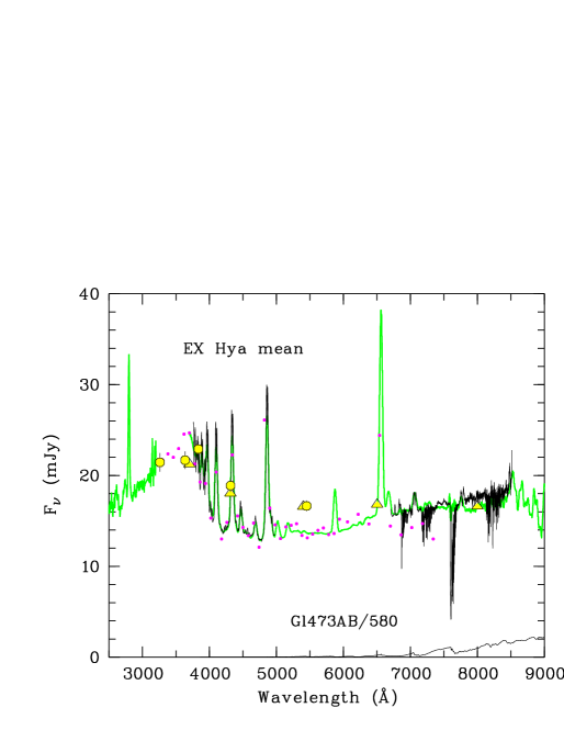
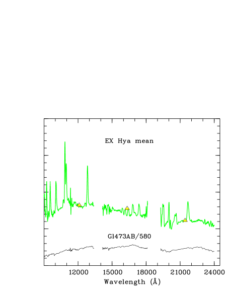
Figure 1: Flux calibrated spin-averaged blue and red UVES spectra of EX Hya (black curves) superposed on the overall spectral energy distribution of Eisenbart et al. (2002) (green curves). Also shown is the spectrophotometry of Bath et al. (1981) (small dots, see text), the Walraven photometry of (Siegel et al. 1989) (open circles), and unpublished UBVRIJHK photometry (open triangles, see text). Also shown is the optical/infrared spectrum of the dM5.5 star Gl473AB (Eisenbart et al. 2002) adjusted to the flux level of the secondary star in EX Hya.

EX Hya was observed in service mode with the UVES spectrograph at the Kueyen (UT2) unit of the ESO Very Large Telescope, Paranal/Chile, on January 23 and 26, 2004. Table 1 contains a log of the observations. We adopted the ESO UVES pipeline reduction that provides flat fielding, performs a number of standard corrections, extracts the individual echelle orders, and collects them into a combined spectrum. The flux calibration, except for the seeing correction (Sect. 3.2), is also part of the pipeline reduction. The wavelength calibration is derived from spectra taken with a ThAr lamp. Blue and red spectra were measured simultaneously in the wavelength ranges 3760–4980Å and 6706–8521Å with pixel sizes of 0.030 and 0.041Å, respectively. With a slit width of 1″, the FWHM resolution is 0.175Å and the spectral resolution is $\lambda/\Delta\lambda\simeq 47\,000$. To improve the S/N ratio, we rebinned the data into 0.3Å bins ($\sim 10$ km s^-1) and obtained an effective resolution $\lambda/\Delta\lambda\simeq 27\,000$. Exposure times were 300 s with dead times of typically 60 s between exposures due to readout. The resulting orbital phase resolution is $\Delta\phi_{98}=0.061$, the spin phase resolution is $\Delta\phi_{67}=0.090$. For the subsequent analysis, we combined the data of both nights into 16 orbital phase bins.

Figure 1 (left panel) shows the flux calibrated and spin-averaged blue and red UVES spectra of EX Hya before the correction for telluric-line absorption. The spectra are overlaid on the spin-averaged spectral energy distribution from Eisenbart et al. (2002) and the spectrophotometry of Bath et al. (1981). The latter is converted from spin phase $\phi_{67}$=0.15 to 0.25 (i.e., to spin average) using the known wavelength dependence of the spin modulation. Also shown is the Walraven photometry of Siegel et al. (1989) and the spin averages of unpublished phase-resolved simultaneous UBVRIJHK photometry taken in 1982 by Joachim Krautter and Nikolaus Vogt (private communication). The flux level of the mean red UVES spectrum agrees with the earlier data to better than 10%, whereas a wavelength-dependent correction between -5% and 20% was needed to adjust the mean blue UVES spectrum to the Eisenbart et al. and the Bath et al. spectrophotometry. The high degree of internal consistency between the various measurements provides confidence in the flux calibration of the red UVES spectra discussed in this paper.

Spectra of the M4.25 dwarf Gl300 were taken with the same setup on January 29. A UVES spectrum of the M6 dwarf Gl406, more akin to the secondary star in EX Hya than Gl300, was kindly provided by Ansgar Reiners. Flux calibrated red spectra of these M-stars (corrected for telluric lines) are displayed in Fig. 2. The gap in the Gl406 UVES spectrum between 8190 and 8403Å is filled in with a medium-resolution archival spectrum of ours (dotted curve). The red spectrum of Gl300 fits the Kron-Cousins $I_{\mathrm{c}}$-band photometry ($I_{\mathrm{c}}=9.17$, Leggett 1992) without any adjustment confirming the accuracy of the UVES flux calibration, whereas the blue spectrum shows a similar moderate loss of blue light as noted above. The Gl406 spectrum is adjusted to $I_{\mathrm{c}}=9.39$ (Leggett 1992). As discussed below, the secondary star in EX Hya is of spectral type dM5 to dM6 and contributes about 5% of the mean flux of EX Hya at 7500Å. The correspondingly adjusted spectrum of the dM5.5 star Gl473AB (Eisenbart et al. 2002) illustrates the dominance of the disk and funnel emission in EX Hya (Fig. 1).

Figure 2: Flux calibrated red UVES spectra of the M6 dwarf Gl406 and the M425 dwarf Gl300 (shifted upwards by two units). The ’residual’ spectra shown as the two bottom curves refer to our method of analyzing the EX Hya spectra and are explained in Sect. 3.3. The bottom one refers to Gl406 and is shifted downwards by one unit.

3 Data Analysis

In this section, we discuss the accuracy of the wavelength calibration, outline the seeing correction that is part of the flux calibration, and discuss the correction of the individual red spectra for telluric line absorption.

3.1 Wavelength calibration

The UVES pipeline reduction provides wavelength-calibrated spectra. The accuracy of this wavelength calibration can be verified in the red spectral region by measuring the positions of the numerous telluric lines of $\mathrm{O}_{2}$ and $\mathrm{H}_{2}\mathrm{O}$. As an example, Fig. 3 shows the water vapor lines near 8200Å. Comparison of theoretical and observed positions of unblended lines with moderate optical depths yield a mean difference in these positions of $\Delta\lambda=3\pm 3$ mÅ throughout the red spectral range and a standard deviation of $\sigma=13$ mÅ. Hence, the wavelength calibration is quite accurate and the systematic error in the derived radial velocities does not exceed 1.0 km s^-1.

3.2 Seeing correction

Seeing information is provided by the DIMM on Paraneal (Difference Image Motion Monitor, Sarazin & Roddier 1990) and by the width of the individual spectral images perpendicular to the dispersion direction. Both methods yielded compatible estimates of the FWHM seeing that varied between 0.9″ and 2.2″ on January 23 and between 0.7″ and 1.2″ on January 26. We corrected each spectrum for the seeing losses assuming a Gaussian point spread function and a central position of the source in the 1.0 arcsec slit. This correction is part of our flux calibration and is included whenever we quote absolute fluxes. In particular, this holds for the spectra in Fig. 1 and for the light curves shown in Fig. 4 and discussed in Sect. 4.4, below.

Figure 3: Mean normalized spectrum of EX Hya in the vicinity of the NaI$\lambda 8183/8195$ doublet. Wavelength bins are 41 mÅ and the FWHM spectral resolution is 175 mÅ. The two spectra shown at the top are explained in Sect. 3.3. The NaI doublet becomes detectable only after telluric correction.

3.3 Telluric line correction

We reconstruct the stellar flux incident on the atmosphere by correcting the observed spectra for the absorption in the telluric lines. Given the structure of the spectrum as shown in Fig. 3, this is a formidable task, in particular, since the water vapor content of the atmosphere on January 23 and 26, 2004, was rather high. Absorption in the strongest $\mathrm{H}_{2}\mathrm{O}$ lines near 8200Å reached 88%, whereas the depth of the NaI$\lambda 8183/8195$ doublet is only 2.6% of the continuum.

Telluric correction of the observed spectrum $F_{\mathrm{i}}(\lambda)$ of orbital phase bin $i$ requires division by $\mathrm{exp}({-\tau_{\mathrm{i}}(\lambda)}$), where $\tau_{\mathrm{i}}(\lambda)$ is the wavelength dependent optical depth of the atmosphere. We need to define a template $\tau(\lambda)$ that allows us to construct the individual $\tau_{\mathrm{i}}(\lambda)$ and to reach the desired accuracy of the reconstructed fluxes. To start with, we employed the normalized spectrum of a featureless standard star obtained in a different night as template $\tau(\lambda)$. This proved unsuccessful, because the optical depth in water vapor was only about 1/3 of that in our observations and the optical depth structures did not match. We resorted, therefore, to an entirely different method using the orbital mean red spectrum of each night as a telluric template. At first glance, this might seem inappropriate, because it removes all spectral structure from the mean of our set of phase-resolved spectra. For the special case of a cataclysmic variable with its rapid variability, the method is attractive, however, because it removes all spectral structure that does not display orbital (or more generally temporal) variability. Although the mean spectrum vanishes, the individual corrected exposures that we refer to as ’residual’ spectra retain much of the spectral structure at wavelength scales less than that of the radial velocity variation of $\sim 20$Å in case of EX Hya.

To explain the method, we present a model calculation with the 4-Å binned spectra of Gl300 and Gl406 shown in Fig. 2. Let $F(\lambda)$ be the spectrum of the M-star and $F_{\mathrm{i}}(\lambda)$ the same spectrum for orbital phase bin $i$ shifted in wavelength according to the radial velocity of the secondary star in EX Hya. The mean of $N$ phase bins is $\overline{F}(\lambda)=(1/N)\sum_{1}^{N}F_{\mathrm{i}}(\lambda)$ and the residual spectra are $f_{\mathrm{i}}(\lambda)=F_{\mathrm{i}}(\lambda)-\overline{F}(\lambda)$. Figure 2 (bottom curves) shows the residuals of Gl300 and Gl406 at orbital phase $\phi_{\mathrm{98,\,i}}=\,0.75$, calculated for an orbital velocity amplitude of 432.4 km s^-1 and a spectral flux that does not vary with phase. Spectral structure that extends over $\Delta\lambda>20$Å is lost, while structure on a shorter scale is preserved with an amplitude up to 90% of the original.

Figure 4: Flux-calibrated light curves of EX Hya obtained on January 23, 2004. The bands $U^{\prime}$ and $B$ refer to the mean flux in the intervals 3770–4000Å and 4000–4800Å, respectively. The integrated flux of the H$\beta$ emission line is given in units of $10^{-13}$ erg cm^-2s^-1. The triangles indicate the times of spin maxima predicted by the quadratic ephemeris of Hellier & Sproats (1992).

For EX Hya, we express the ’raw’ spectrum $F_{\mathrm{i}}(\lambda)$ of orbital phase bin $i$ as

$$F_{\mathrm{i}}(\lambda)=C_{\mathrm{i}}(\lambda)\,n_{\mathrm{i}}(\lambda),$$ (1)

where $C_{\mathrm{i}}(\lambda)$ represents the smooth wavelength dependence of the continuum and $n_{\mathrm{i}}(\lambda)$ is the normalized spectrum that contains all spectral structure. We use the orbital mean of the $n_{\mathrm{i}}(\lambda)$ as the telluric template $\overline{n}(\lambda)\equiv\mathrm{exp}(-\tau(\lambda))$. The correction function for phase bin $i$ is calculated as $\mathrm{exp}(-\tau_{\mathrm{i}}(\lambda))=\mathrm{exp}(-\alpha_{\mathrm{i}}\tau(\lambda))=\overline{n}(\lambda)^{\,\alpha_{\mathrm{i}}}$ with a parameter $\alpha_{\mathrm{i}}$ that is independent of wavelength. We determine the $C_{\mathrm{i}}(\lambda)$ by fitting a low-order polynomial to the continuum of the raw spectra. The template is then fitted to the resulting $n_{\mathrm{i}}(\lambda)$ over a specified spectral range allowing for a small wavelength shift $\delta\lambda_{\mathrm{i}}$ (of order mÅ). Hence, the residual spectrum for phase bin $i$ is

$$f_{\mathrm{i}}(\lambda)=F_{\mathrm{i}}(\lambda){[\,\overline{n}\,(\lambda+\delta\lambda_{\mathrm{i}})]^{-\alpha_{\mathrm{i}}}}-C_{\mathrm{i}}(\lambda)\leavevmode\nobreak\ ,$$ (2)

with fit parameters $\alpha_{\mathrm{i}}$ and $\delta\lambda_{\mathrm{i}}$. In our data, the optical depth varies little with orbital phase and the $\alpha_{\mathrm{i}}$ stay close to unity. We define the continua $C_{\mathrm{i}}(\lambda)$ by quadratics fitted to the $F_{\mathrm{i}}(\lambda)$ at 6800Å, 7720Å, and 8362Å for $\lambda<8000$Å and at 7130Å, 7854Å, and 8362Å for $\lambda>8000$Å. At these wavelengths, any temporal variation of the spectral flux is removed and the residual spectra equal zero. Any remaining orbital modulation of the residual flux is relative to these wavelengths. Telluric absorption is considered separately for absorption by $\mathrm{O}_{2}$ and $\mathrm{H}_{2}\mathrm{O}$ lines. The template is fitted to the $\mathrm{O}_{2}$ lines between 7620Å and 7657Å avoiding the KI lines and the deepest part of the A-band at 7593–7617Å. It is fitted to the $\mathrm{H}_{2}\mathrm{O}$ lines over the bands 8000-8150Å and 8220–8350Å avoiding the NaI doublet. We restrict the subsequent analysis to $\lambda>7300$Å and piece the residual spectra together from the $\mathrm{O}_{2}$-corrected part below 8000Å and the $\mathrm{H}_{2}\mathrm{O}$-corrected part above 8000Å. The two fits remove the weaker telluric lines outside the immediate fit intervals almost perfectly and only the 7593–7617Å section remains problematic, where absorption at the line centers reaches 99.8%. The spectra of both nights are then combined and collected into 16 phase bins. The result is shown in Fig. 5. Spectral structure on a short wavelength scale is preserved in the individual reconstructed spectra although they average to zero.

3.4 Statistical noise

A natural consequence of any telluric-line correction is the increased noise level of the restored fluxes at the positions of the strong lines. We opted to keep all data points in the resulting spectra and account for the enhanced noise at the telluric line positions by the increased statistical errors of the affected data points. The orbital mean of the reconstructed normalized spectra for the first night is shown in Fig. 3 (second curve from top, shifted upwards by 0.2 units). As expected, it equals unity with only minute deviations that disappear, too, when it is rebinned to 0.3Å. The statistical error of the individual 0.3Å spectral bins is determined from the mean rms noise in regions that avoid the strongest telluric lines and amounts to 0.7% of the continuum (Fig. 3, uppermost curve). It reaches 2% in the deepest $\mathrm{H}_{2}\mathrm{O}$ lines around 8200Å and huge values in the deepest lines of the A-band between 6593 and 7617Å. The 0.7% level corresponds to an absolute error of $6\times 10^{-17}$erg cm^-2s^-1Å^-1 near 8200Å.

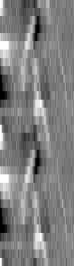
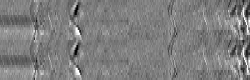
Figure 5: Phase-resolved and telluric line-corrected ’residual’ spectra of EX Hya collected into 16 phase bins and repeated for two orbits (see Sect. 3.3). Numerous emission and absorption features from the secondary star are visible, most prominent the TiO band heads at 7589 and 8432Å, the KI$\lambda 7665/7699$ and NaI$\lambda 8183/8195$ emission/absorption lines, and CaII$\lambda 8498$ in emission. The broad HeI, OI, and Paschen lines are from the accretion disk and funnel. The displayed intensities are relative to the orbital mean, the zero level is shaded gray, lower and higher intensities appear darker and lighter, respectively.

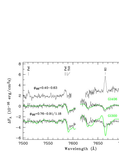
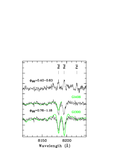
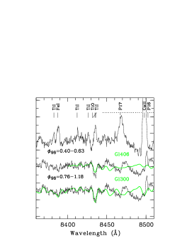
Figure 6: Absolute ’residual’ spectral fluxes $f_{\mathrm{i}}(\lambda)$ of EX Hya for the illuminated face of the secondary star (top, black data train, shifted upwards by three units) and its dark side (center and bottom, black data train, unshifted and shifted downwards by three units, respectively). The spectra are shifted in wavelength to the respective rest frame before averaging them over the orbital phase intervals indicated in the figure (see text). Shown for comparison are the correspondingly constructed ’residual’ fluxes of the M6 dwarf Gl406 and the M4.25 dwarf Gl300.

4 Observational results

The gray plots of Fig. 5 show the 16 phased-resolved residual spectra for the wavelength intervals 4875–4975Å and 7300–8520Å displayed twice. The wavelength bins are 0.3Å. In the selected spectral ranges, the strongest broad emission lines from the accretion disk and funnel are HeI$\lambda 4922$, OI$\lambda 7772/7774/7775$, Paschen P17, CaII$\lambda 8498$, and Paschen P16. The narrow spectral features from the secondary star include the TiO band heads at 7589Å and 8432Å, the KI$\lambda 7665/7699$ and the NaI$\lambda 8183/8195$ lines in absorption and emission, CaII$\lambda 8498$ in emission, and numerous metal emission lines, among the stronger ones FeI$\lambda 4957$, FeI$\lambda 8327$ and FeI$\lambda 8388$. The absorption lines are strong between $\phi_{98}$ = 0.65 and 1.35, whereas the emission components reach peak flux at $\phi_{98}$ $\simeq 0.50$, both indications of an origin from the illuminated secondary star. The narrow and strong CaII$\lambda 8498$ emission line is superimposed on a complex background of the much broader Paschen P16, P17, and CaII$\lambda 8498$ disk lines. We have separated the narrow line interactively from the background and included an estimate of the uncertainty of this procedure in the errors of the individual data points.

4.1 The secondary star in EX Hya

Figure 6 displays mean spectra for the phases when the illuminated face of the secondary star or its dark side are in view (black curves). The spectra are summed over the respective phase intervals, are placed on an absolute flux scale, and shifted into the rest systems of the emission or the absorption lines, respectively. To appreciate the weakness of the lines note that the depth of the NaI doublet is 2.6% of the continuum at 8200Å (Fig. 1). Information on the spectral type of the secondary star in EX Hya can be obtained from a comparison of these spectra with those of the M-stars Gl300 and Gl406 (green curves). We have used the M-star spectra at their full spectral resolution, adjusted their fluxes with the ratio of the solid angles $\Omega$,

$$F_{\mathrm{sec}}=F_{\mathrm{M}}\,\Omega_{\mathrm{sec}}/\Omega_{\mathrm{M}}=F_{\mathrm{M}}(R_{\mathrm{sec}}/d)^{2}(d_{\mathrm{M}}/R_{\mathrm{M}})^{2},$$ (3)

formed the residuals as explained in Sect. 3.3, and rebinned them to 0.3Å. Here, $d_{\mathrm{M}}$ and $R_{\mathrm{M}}$ are the distance and the stellar radius of the M-star (Beuermann et al. 1999), whereas $d=(64.5\pm 1.2)$ pc (Beuermann et al. 2003) and $R_{\mathrm{sec}}=(0.1516\pm 0.0034)\,R_{\odot}$ (see Sect. 6.3, below) denote the distance of EX Hya and the mean radius of its secondary, respectively. The ratio of the solid angles amounts to $\Omega_{\mathrm{sec}}/\Omega_{\mathrm{M}}=0.00421\pm 0.00036$ for Gl300 and $\Omega_{\mathrm{sec}}/\Omega_{\mathrm{M}}=0.00170\pm 0.00015$ for Gl406. The residual spectrum of the dark side of EX Hya is displayed twice in the three panels of Fig. 6, at the center and the bottom. For $\lambda<7605$Å, we have chosen the phase interval $\phi_{98}$=0.76–0.91, when the emission lines have already disappeared and the blueshift has moved the TiO band head at 7589Å away from the telluric A-band. For $\lambda>7615$Å, we sum over the entire dark side of the secondary ($\phi_{98}$=0.76 – 1.18). Our comparison indicates that the residual spectrum of Gl406 reproduces the TiO band head of EX Hya at 7589Å perfectly. The KI lines of Gl406 fit almost as well, whereas those of Gl300 utterly fail. The NaI doublet suggests a spectral type between Gl300 and Gl406 and the TiO band head at 8432Å prefers Gl300. Many of the low-amplitude wiggles in the EX Hya spectrum faithfully reproduce rotationally smoothed absorption line structures of the two M-stars. This agreement is lost for $\lambda>8445$Å, where the broad disk lines veil the spectral features of the secondary star. The TiO band head at 8432Å is also affected by the two flanking TiI emission lines and, assigning it a lower weight, we conclude that the EX Hya spectrum is much better represented by Gl406 (dM6) than by Gl300 (dM4.25). The implied spectral type of the secondary is slightly earlier than M6 and we settle for dM$5.5\pm 0.5$. Interpolating between the adjusted fluxes of Gl300 and Gl406, we find that the the secondary contributes $0.92\pm 0.28$ mJy and $1.40\pm 0.48$ mJy at 7500Å and 8200Å, respectively. This corresponds to $(5.3\pm 1.6)$% and $(7.5\pm 2.6)$% of the spin-averaged flux of EX Hya, respectively (see Fig. 1).

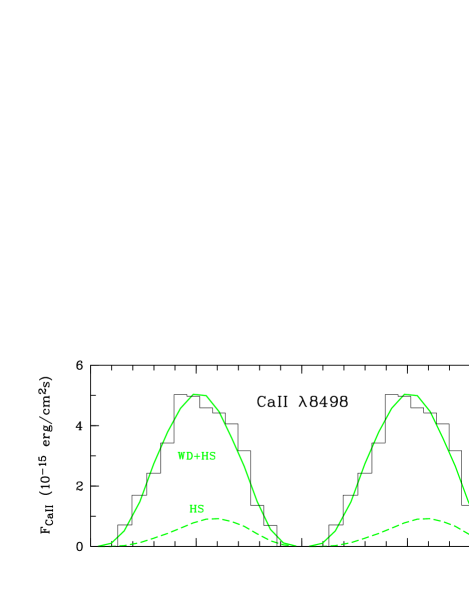
Figure 7: Top: Orbital light curve of the CaII$\lambda 8498$ integrated emission line flux (black histogram) and model fit (green curves). The two components refer to the white dwarf (WD) and the hot spot (HS) as irradiation sources. Bottom: Flux at 7550Å relative to 7720Å. The dip indicates a weakening of the TiO$\lambda 7589$ band strength on the illuminated face of the secondary star. The abscissa is orbital phase calculated from Eq. 4.

Although the dark side of the secondary looks like a dM5.5 star, this does not hold for the illuminated side as shown by the spectrum for $\phi_{98}$= 0.40–0.63 in Fig. 6 (top). This phase interval is characterized by the peak flux of the emission lines and a disappearance of the TiO$\lambda 7589$ absorption edge. Figure 7 shows the light curves of the integrated flux of the CaII$\lambda 8498$ emission line (upper panel) and the difference $\Delta F_{7550}$ of the residual fluxes at 7550 and 7720Å (lower panel). The minimum of the latter coincides with the emission line maximum stressing the weakness of the TiO$\lambda 7589$ band head on the illuminated face, a result that is reminiscent of Wade & Horne’s (1988) finding for Z Cha.

Applying Eq. (3) to the $K$-band, allows us to estimate the contribution of the secondary to the infrared flux of EX Hya. The apparent $K$-band magnitudes of Gl300 and Gl406, $K=6.68$ and 6.08, imply $K_{\mathrm{sec}}=12.62$ and 13.00 for a secondary of spectral type dM4.25 or M6, respectively. For the preferred spectral type dM$5.5\pm 0.5$, EX Hya B has $K_{\mathrm{sec}}=12.89\pm 0.11$. We can alternatively start from the surface brightness calibration of field M-dwarfs by Beuermann (2006) that implies $S_{\mathrm{K}}=4.71\pm 0.11$ for a spectral type dM$5.5\pm 0.5$. With $R_{\mathrm{sec}}=(0.1516\pm 0.0034)\,R_{\odot}$ and $d=(64.5\pm 1.2)$ pc, we find $K=S_{\mathrm{K}}-5\,\mathrm{log}[(R_{\mathrm{sec}}/R_{\odot})(10\mathrm{pc}/d)]=12.86\pm 0.13$, nearly identical with the previous number. The absolute magnitude of the secondary in EX Hya is $M_{\mathrm{K}}=8.83\pm 0.12$, in perfect agreement with that of a main sequence dM5.5 star. The spin-averaged apparent $K$-band magnitude of EX Hya is $K=11.81$ (Fig. 1) to which the secondary contributes $(37.6\pm 4.2)$%, somewhat less than estimated by Eisenbart et al. (2002). These authors noted already that part of the modulation of the infrared bands at one half the orbital period that looks like the ellipsoidal modulation of the secondary star may be produced by the bulge on the accretion disk. We confirm this suspicion by noting that the optical bands of the unpublished UBVRIJHK photometry (Sect. 2) display a 49-min modulation, too.

4.2 Radial velocity amplitudes and systemic velocity

The brightest emission lines suited for radial velocity measurements are CaII$\lambda 8498$, KI$\lambda 7665/7699$, FeI$\lambda 8327$, and FeI$\lambda 4958$. Of the absorption lines, only the NaI$\lambda 8183/8195$ doublet yields reliable results. In KI$\lambda 7665/7699$, the emission component is relatively stronger and the profiles are affected by residuals of the telluric $\mathrm{O}_{2}$ lines. In this initial analysis, we measured radial velocities using Gaussians for the single lines and a double Gaussian with a separation of 11.57Å for the NaI doublet. Figure 8 shows the radial velocity curves of the CaII emission line measured from the 48 individual exposures and of the NaI doublet measured from the 16 phase-binned spectra. The abscissa $\phi_{\mathrm{98,HS}}$ is the orbital phase calculated from the linear ephemeris of Hellier & Sproats (1992). The NaI absorption component is disturbed by emission on the descending branch and becomes undetectable around $\phi_{98}\simeq 0.5$. We have measured the velocity amplitudes, the phase shifts, and the systemic velocities from sinusoidals fitted to all data points for the emission lines and to the data points between $\phi_{\mathrm{98,HS}}=0.71$ and 1.21 for NaI. The fit results are listed in Tab. 2. Although these fits do not account for the slight ellipticity visible in the data, they yield quite accurate values of the velocity amplitudes $K_{2}^{\prime}$ of the emission lines and of the systemic velocity $\gamma$. Neither the emission lines with an average $K_{2}^{\prime}=351$ km s^-1 nor the NaI absorption lines with $K_{2}^{\prime\prime}=460$ km s^-1 provide a reliable measure of the velocity amplitude $K_{2}$ of the secondary star, which we expect to fall in between. Note that the TiO$\lambda 7589$ band head is not suited to track the motion of the secondary star, because it is disturbed by the A-band around $\phi_{98}$=0.25 and by FeI$\lambda 7584/7586$ emission between $\phi_{98}$=0.2 and 0.8.

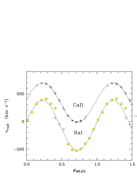
Figure 8: Radial velocity curves of NaI$\lambda 8183/8195$ in absorption ($\medcirc$) and emission ($+$) (left hand scale) and of the CaII$\lambda 8498$ emission line ($+$) (right hand scale) vs. orbital phase $\varphi_{\mathrm{98,HS}}$ (Hellier & Sproats 1992). Solid lines represent sinusoids least squares-fitted to the data (see Sect. 4.2). The error bars are smaller than the data points.

The systemic velocities of the individual lines in Tab. 2 are generally in good agreement, although the NaI absorption line value may be affected by the emission component and the first KI value by possible blending with FeI at 7664.29Å. Excluding these, the mean systemic velocity of the remaining four lines becomes $\gamma=-59.0\pm 0.9$ km s^-1. The small systematic error of our wavelength calibration adds only 0.5 km s^-1 to the error budget of $\gamma$ (see Sect. 3.1). Confirmation on the common origin of all narrow emission lines and on the value of $\gamma$ is obtained from the numerous lines seen in the blue spectra. They originate from neutral or singly ionized species and are restricted to the phase interval when the illuminated face of the secondary is in view. The better defined ones with equivalent widths between 0.04Å and 0.11Å are HI$\lambda 3770,3797,4102$, FeI$\lambda 3856,3889,4198,4271,4314,4426,4890,4957$, CaII K, MnI$\lambda 4034$, ArI$\lambda 4045$, OII$\lambda 4144$, NaI$\lambda 4216$, NeII/AlII$\lambda 4227$, OI$\lambda 4232$, NeI$\lambda 4274$, CrI$\lambda 4583$, and MgII$\lambda 4938$. Narrow emission components are not detected in the HeI lines and in HeII$\lambda 4886$. We have studied these faint lines in a cursory manner shifting them into their rest system with an appropriate $K_{2}^{\prime}$. We obtain straight vertical lines in the 2-D image for the $K_{2}^{\prime}$ value of the red lines, 351 km s^-1. The systemic velocities are measured from a spectrum co-added over the phase interval of best visibility of the lines. Their distribution has a standard deviation of $\sigma=2.3$ km s^-1 and a mean $\gamma=-59.6$ km s^-1, indistinguishable from that of the red lines.

Table 2: Results for sinusoidal fits $\upsilon_{\mathrm{rad}}=K\,\mathrm{sin}[2\pi(\phi_{98}+\phi_{0})]+\gamma$  to the radial velocities of narrow emission lines and the NaI absorption line doublet. The errors in brackets refer to the last digit. See text for systematic errors.

Ion	$\lambda$	$K$	$\phi_{0}$	$\gamma$	Line
	(Å)	(km s-1)		(km s-1)
FeI	4957.58	$343\pm 8$	0.014(5)	$-60\pm 4$	em
KI	7664.90	$351\pm 5$	0.021(3)	$-65\pm 4$	em
KI	7698.96	$358\pm 5$	0.021(3)	$-61\pm 4$	em
FeI	8327.05	$345\pm 5$	0.019(3)	$-58\pm 5$	em
CaII	8498.02	$357\pm 3$	0.020(4)	$-57\pm 5$	em
NaI	8183.26/8194.82	$460\pm 5$	0.021(2)	$-68\pm 3$	abs

Unfortunately, there are no accurate previous measures of $\gamma$ from optical lines to compare our result with, except the rather uncertain values quoted by Hellier et al. (1987). It is potentially important, however, to note the more positive $\gamma$ velocities derived from UV and X-ray emission lines that originate near the white dwarf surface, $\gamma=9.5\pm 3.0$ km s^-1 (Belle et al. 2005) and $\gamma=-2.8\pm 2.3$ km s^-1 (Hoogerwerf et al. 2004). The errors quoted by these authors are statistical ones and additional systematic errors may affect the numbers. Nevertheless, it is interesting to note that the difference between the optical and X-ray/UV results is close to the gravitational redshift expected for the white dwarf in EX Hya (see Sect. 7).

4.3 Check on the origin of the narrow emission lines

Belle et al. (2003) and Hoogerwerf et al. (2004) have reported accurate values of the radial velocity amplitude of the white dwarf, $K_{1}=59.6\pm 2.6$ km s^-1 and $K_{1}=58.2\pm 3.7$ km s^-1, respectively. We show here that the fully resolved profiles of the narrow optical lines in our spectra independently yield a very similar, although not quite as accurate value of $K_{1}$. To this end, note that the measurement of two velocity amplitudes that can be assigned to two points on the line connecting the two stars is equivalent to the measurement of the radial velocity amplitudes of both stars: we choose the back of the Roche lobe and the L₁ point. The peak velocity in the NaI absorption line profile at quadrature corresponds to the velocity amplitude of the back of the star if we account for some widening by pressure broadening. We choose a point two pixels (20 km s^-1) down into the absorption line profile and obtain $K_{\mathrm{back}}=550\pm 10$ km s^-1. The minimum velocity in the CaII emission line profiles at quadrature is taken to represent the L₁ point. Since the emission lines display no additional broadening, we choose the first pixel in the CaII line profiles with a non-vanishing flux and obtain $K_{\mathrm{L1}}=280\pm 10$ km s^-1. The ratio of these velocities equals $K_{\mathrm{back}}/K_{\mathrm{L1}}=x_{\mathrm{back}}/x_{\mathrm{L1}}=1.96\pm 0.08$, with $x_{\mathrm{back}}$ and $x_{\mathrm{L1}}$ the coordinates along the $x$-axis of the two extremal points on the stellar surface as measured from the center of gravity in units of the binary separation. Roche geometry then implies $q=M_{2}/M_{1}=0.134\pm 0.019$, $x_{\mathrm{back}}=1.129\pm 0.005$, $K_{2}=K_{\mathrm{back}}/x_{\mathrm{back}}/(1+q)=430\pm 9$ km s^-1, $K_{1}=qK_{2}=58\pm 8$ km s^-1, and $K_{1}+K_{2}=488\pm 9$ km s^-1. With the orbital period $P_{\mathrm{orb}}$=5895.4 s and the inclination $i=77.8^{\circ}$, the binary separation is $a=(K_{1}+K_{2})P_{\mathrm{orb}}/(2\pi\mathrm{sin}i)=(4.683\pm 0.088)10^{10}$cm. Finally, Kepler’s law gives a total mass of $M=0.88\pm 0.05$ M_⊙ and component masses $M_{1}=0.775\pm 0.045$ M_⊙ and $M_{2}=0.104\pm 0.016$ M_⊙. Since $K_{\mathrm{back}}$ and $K_{\mathrm{L1}}$ were simply read from the observed profiles, these numbers are approximate only. The important point to note is the excellent agreement between our value of $K_{1}$ and the directly measured, more accurate radial velocity amplitude of the white dwarf quoted at the top of this paragraph. This agreement verifies our assumption that the low-velocity limit in the CaII line profiles at quadrature measures the motion of matter that is located on the secondary star near L₁. This assumption forms the basis of the line synthesis procedure described in Sect. 5, below.

Table 3: Barycentric timings of the spin maxima (spin phase zero), the eclipse center, and the zero crossing of the absorption lines from the secondary star (orbital phase zero). The O–C values are given relative to the ephemerides of Hellier & Sproats (1992) (see text).

Band	HJD+2400000	Error	O–C
	(d)	(d)	(d)
(a) Spin maxima
Blue light	53027.7670	0.0014	0.0113
	53027.8109	0.0014	0.0087
	53030.8381	0.0014	0.0104
H$\beta$ flux	53027.7640	0.0014	0.0083
	53027.8109	0.0014	0.0087
	53030.8360	0.0014	0.0083
(b) Eclipse timing
Blue light, H$\beta$ flux	53030.7909	0.0014	$-0.0004$
(c) Absorption line zero crossing
NaI doublet	53030.7893	0.0001	$-0.0012$

4.4 Phase shifts

All photometrically determined eclipse timings reported over the last decade occur near a Hellier & Sproats (1992) orbital phase $\phi_{98,HS}\simeq 0.98$. The blue-to-red zero crossing of the NaI line in our data takes place at $\phi_{98,HS}=0.982\pm 0.001$ (Tab. 3) indicating that eclipse and zero crossing coincide within about the jitter in the eclipse timings (e.g. Siegel et al. 1989). This is confirmed by one pronounced dip that is superimposed on the first spin maximum in the night of January 26, 2004, occurs at spectroscopic phase zero within the error, and probably represents the eclipse by the secondary star (Tab. 3).

The spin light curves in Fig. 4 show that blue light, red light, and the H$\beta$ flux display the same spin modulation within errors. The U’, B and 7500Å bands are integrals over 3760–4000Å, 4000–4800Å, and 7450–7550Å, respectively. The H$\beta$ flux is an average over $\pm 40$Å of the line center corrected for the underlying continuum. The solid triangles on the abscissa indicate the times of the spin maxima predicted by the quadratic ephemeris of Hellier & Sproats (1992). The offset between observed and calculated times of maxima is $\Delta\phi_{67}=-0.20\pm 0.03$ and, in what follows, we use the phase conventions

$$\phi_{98}=\phi_{98,HS}+0.018\qquad\mathrm{and}\qquad\phi_{67}=\phi_{67,HS}-0.20.$$ (4)

Irradiation of the secondary star in EX Hya varies periodically at the beat period between orbital and rotational periods (210 min) and inclusion of Eq. (4) into our illumination model assures correct phasing. The only other post-1991 timings of blue light maxima that we are aware of are those by Eisenbart et al. (2002), $\Delta\phi_{67}=-0.04\pm 0.01$ at HJD 2450508, and Belle et al. (2005), $\Delta\phi_{67}=-0.12\pm 0.02$ near HJD 2451685. Although substantial fluctuations occur in the timings (Hellier & Sproats 1992; Belle et al. 2005), the numbers suggest that the offset increases with time and that the spin-up of the white dwarf in EX Hya is slightly slower than quoted by Hellier & Sproats (1992). A more regular monitoring of EX Hya with a small telescope a worthwhile undertaking.

5 Irradiation model

We now embark on the construction of a detailed line synthesis model for NaI$\lambda 8183/8195$ and CaII$\lambda 8498$. Our model represents the Roche lobe by a grid of triangular surface elements, each of which is characterized by photospheric absorption and potentially by superimposed emission from a thin layer that we do not distinguish geometrically from the photosphere.

5.1 Line profiles

Velocity smearing is adopted as the dominant broadening mechanism, supplemented by pressure broadening for the NaI absorption lines and minimal Gaussian broadening of the CaII emission line. Pressure broadening is represented by a Lorentz profile derived from the NaI doublet in the M4.25 dwarf Gl300. The emission lines, on the other hand, are produced in layers above the photosphere and probably lack significant pressure broadening. The adopted Gaussian broadening with a FWHM of one pixel (10 km s^-1) merely serves to smooth irregularities arising from the 0.01 phase bins of the model spectra.

In principle, modeling the complex line profiles that contain absorption and emission components requires appropriate radiative transfer calculations for irradiated M-dwarf atmospheres (Brett & Smith 1993; Barman et al. 2004). Results that could easily be implemented are not yet available, however, and we consider two simple cases instead: (i) the fill-up of the absorption line with emission by adding the two components; and (ii) the gradual disappearance of the absorption line in the illuminated part and its replacement by emission. The difference lies in the absorption line wings that are retained in case (i) and practically disappear in case (ii). Testing both models led to better fits with and a clear preference for case (i) (see Fig. 14, top). The adopted procedure is adequate for the present data, but may have to be replaced by a more sophisticated approach if data of better statistical accuracy become available.

5.2 Parameterization of the model

Our kinematic and illumination model has 29 parameters of which 24 are listed in Tab. 4 and the remaining five are normalization constants explained in Sect. 5.4. Parameters that are kept fixed are the orbital period $P_{\mathrm{orb}}$, the inclination $i$, the phase shift $\Delta\phi_{67}$, the 210-min amplitude of the irradiation flux $A_{\mathrm{irr}}$, the optical depth of the emitting layer on the secondary $\tau$, the intrinsic FWHM of the line emission, the NaI gravity darkening coefficient $y_{\lambda}$, and the constants $c$ and $d$ in the NaI limb darkening law (all explained either above or in the next two Sections). We opted to provide the white dwarf radial velocity amplitude $K_{1}\simeq 59\pm 3$ km s^-1 (Belle et al. 2003; Hoogerwerf et al. 2004) as a fixed input parameter and determine its influence on the errors of the fit parameters by varying it between 56 and 62 km s^-1. The mass ratio $q$ is then a derived parameter and is determined as $q(M,K_{1})$. Of the free parameters, the quantities $M$, $\gamma$, and $\Delta\phi_{98}$ describe system properties, whereas the disk half thickness $\beta$, the limit of illumination at $c_{\mathrm{lim}}$, the limb darkening/brightening coefficient of the CaII emission $u_{\mathrm{l,Ca}}$, the eight numerically given CaII emissivities (or one parameter of the analytical model), and the five normalization constants define the emission line model and are discussed in Sect. 5.4. For the numerical or analytical versions of the emission model, 19 or 12 parameters, respectively, are fitted.

Table 4: Parameters of the irradiation model for EX Hya and results of the combined least-squares fit to the NaI$\lambda 8183/8195$ and the CaII$\lambda 8498$ line profiles in 16 orbital phase bins.

No.	Parameter	Symbol	free /	Value $\pm$ Error
			fixed
(a) System parameters:
P1	Orbital period (s)	$P_{\mathrm{orb}}$	fixed	5895.4
P2	Inclination	$i$	fixed	$77.8\pm 0.4^{\circ\leavevmode\nobreak\ 1)}$
P3	Velocity amplitude (km s-1)	$K_{1}$	fixed	$59.0\pm 3.0^{\leavevmode\nobreak\ 2)}$
P4	Total mass (M⊙)	$M$	free	0.898$\pm$0.031
P5	Mass ratio $M_{2}/M_{1}$	$q$		0.137$\pm 0.007^{\leavevmode\nobreak\ 3)}$
P6	System velocity (km s-1)	$\gamma$	free	$-58.2\pm 1.0$
P7	Phase shift	$\Delta\phi_{98}$	free	$0.018\pm 0.001$
P8	Phase shift	$\Delta\phi_{67}$	fixed	$-0.20\pm 0.06$
P9	Ampl. of irradiation flux	$A_{\mathrm{irr}}$	fixed	0.15
(b) NaI$\lambda 8183/8195$ absorption line parameters:
P10	Gravity darkening	$y_{\lambda}$	fixed	0.61
P11	Limb darkening	$c,d$	fixed	see text
(c) CaII and NaI emission line parameters:
P12	Disk half opening angle	$\beta$	free	$2.1^{+1.0}_{-0.5}$
P13	Terminator, cos$\,\vartheta$	$c_{\mathrm{lim}}$	free	$-0.06\pm 0.06$
P14	Optical depth	$\tau$	fixed	$>10$
P15	Limb darkening	$u_{\mathrm{\,l,Ca}}$	free	$0.42\pm 0.24^{\leavevmode\nobreak\ 4)}$
P16	FWHM (km s-1)	$FW$	fixed	10
P17	Normalized CaII	$f_{\mathrm{m}}(\vartheta)$	free	see Fig. 10
…P24	emission line fluxes

¹⁾ From FWHM of the X-ray eclipse for given WD radius $R_{1}(M_{1})$.
²⁾ From (Hoogerwerf et al. 2004; Belle et al. 2003), see text.
³⁾ If $K_{1}$ is fixed in the fit, $q(M,K_{1})$ is not an independent fit parameter.
⁴⁾ Error reflects the strong correlation between $u_{\mathrm{\,l,Ca}}$ and $M$.

5.3 NaI absorption

Limb darkening coefficients are available in the literature only for broad photometric bands. Here, we need the limb darkening of the integrated NaI absorption line flux. We extract this information from the model atmosphere of an unirradiated $\log g$=5 star of 3000 K kindly calculated by Derek Homeier with the PHOENIX code. We determine the mean NaI intensity deficit from the angle-dependent intensity $I_{\lambda}(\mu)$ by integration over the doublet as $I_{\mathrm{Na}}(\mu)=\int_{line}\left(I_{\mathrm{c}}(\mu)-I_{\lambda}(\mu)\right)d\lambda=EW(\mu)\,I_{\mathrm{c}}(\mu)$, where $\mu=\mathrm{cos}\,\theta$ with $\theta$ the zenith angle and $I_{\mathrm{c}}$ denotes the continuum outside the line. Figure 9 shows this quantity normalized to the center of the stellar disk along with a square root fit

$$I_{\mathrm{Na}}(\mu)/I_{\mathrm{Na}}(1)=1-c\,(1-\mu)-d\,(1-\sqrt{\mu}),$$ (5)

(Claret 1998) with parameters $c=-0.069$ and $d=1.063$. The EW of the NaI doublet decreases slightly as the limb is approached and varies approximately as $\mathrm{EW}(\mu)=(6.72+1.07\mu$) Å. The EW averaged over the stellar disk is 7.4Å and both, the $EW$ and the effective temperature of 3000 K, are typical of a dM5.5 star, the best estimate of the spectral type of the secondary star in EX Hya (see Sect. 7 and Tab. 5).

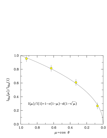
Figure 9: Limb darkening of the angle-dependent intensity deficit integrated over the NaI doublet for a $\log g$=5 star with $T_{\mathrm{eff}}$= 3000 K (Derek Homeier, private communication). The solid line is a fitted square root law with fit parameters $c$ and $d$ given in the text.

We account for monochromatic gravity darkening at 8200Å by a linear coefficient $y_{\lambda}=0.61$ (Tab. 4) that is based on a surface brightness vs. effective temperature relation derived from the results of Beuermann (2006) for field M dwarfs.

Photospheric absorption in the NaI doublet contributed by the $k$-th surface element at orbital phase $\phi_{\mathrm{98,i}}$ is then given by the flux increment

$$dF_{\mathrm{a,k}}=-\,a_{\mathrm{a}}\,dA_{\mathrm{k}}\,\mu_{\mathrm{k}}\,\frac{I_{\mathrm{Na}}(\mu_{\mathrm{k}})}{I_{\mathrm{Na}}(1)}\left(1+2y_{\lambda}(1-\frac{r_{\mathrm{k}}}{R})\right),$$ (6)

with $dA_{\mathrm{k}}$ the surface area of the element, $\mu_{\mathrm{k}}=\mathrm{cos}\theta_{\mathrm{k}}$ and $\theta_{\mathrm{k}}$ the angle between the normal to the element and the line of sight at orbital phase $\phi_{\mathrm{98,i}}$, $r_{\mathrm{k}}$ the radial separation of that element from the center of the star, and $R$ the mean stellar radius. The flux increment is collected into the appropriate 0.3Å wavelength bin that corresponds to the radial velocity of the element as seen by the observer at $\phi_{\mathrm{98,i}}$. For a hidden element with $\mu_{\mathrm{k}}<0$, the flux increment is set to zero. The flux level of the NaI doublet is determined by the fit parameter $a_{\mathrm{a}}$ and a further parameter $a_{\mathrm{ratio}}$ describes the ratio of the $\lambda 8183$ vs. the $\lambda 8195$ lines fluxes.

5.4 CaII and NaI emission

Parameterization of line emission from the irradiated atmosphere is more involved. We model the CaII$\lambda 8498$ emission and adopt its properties for the emission of the NaI doublet with a scaling factor for the different emission line intensities. We assume that the angle-integrated CaII emission line flux $F_{\mathrm{Ca}}$ of surface element depends on its distance $r_{\mathrm{s}}$ from the irradiating source and on the angle of incidence $\vartheta$ as $F_{\mathrm{Ca}}\propto f(\eta)/r_{\mathrm{s}}^{2}$ with $\eta=\mathrm{cos}\,\vartheta$. In the special case of an emitted flux proportional to the incident energy flux, $f(\eta)\propto\eta$. Model calculations for $f(\eta)$ in M-dwarf atmospheres are not yet available, but the case of Lyman line emission of irradiated white dwarf atmospheres (König et al. 2006) suggests that $f(\eta)/\eta$ increases rapidly as grazing incidence is approached ($\eta=0$). We have tested analytical formulations of $f(\eta)$ and a numerical tomographic approach. For the latter, we fix $f(\eta)$ at $f_{1}=0$ for $\eta=0$ (terminator) and at $f_{10}=1$ for $\eta=0.9$ (L₁ point). In between, we define $f(\eta)$ by eight free parameters $f_{\,2}$ to $f_{\,9}$ at equidistant abscissa values $\eta^{\mathrm{(m)}}$. We interpolate between the $f_{\mathrm{m}}$ and regularize the distribution of the emissivities by adding $A\sum_{m=1}^{9}(f_{\mathrm{m+1}}-f_{\mathrm{m}})^{2}$ to the $\chi^{2}$ to be minimized, with $A$ a Lagrange multiplier. This choice implies that a smoothed version of the current set of $f_{\mathrm{m}}$ is used as the default.

The observed light curve of the wavelength-integrated CaII line flux (Fig. 7, upper panel) is slightly skewed with a centroid at orbital phase $\phi_{98}=0.517$. We model this asymmetry by adopting the hot spot or bulge as a second source of irradiation that we locate in the orbital plane at binary coordinates $x=0,y=0.3$ in a system with its origin at the center of gravity, unity separation of both stars along the $x$-axis.

Three further parameters are needed to account for (i) the shadow cast on the secondary by the accretion disk, (ii) a possible horizontal energy transfer across the terminator into the dark side of the star, and (iii) the periodic variation of the irradiation flux received by the secondary from the rotating magnetic white dwarf. We collect these dependencies into three additional parameters: (i) the shadow has a half opening angle $\beta$ independent of azimuth and a sharp edge; (ii) line emission is allowed to extend beyond the geometric terminator for illumination by a point source at $\eta=0$ to $\eta=c_{\mathrm{lim}}$, where $c_{\mathrm{lim}}$ is a small negative (or positive) quantity; and (iii) rotational modulation is modeled by a variation of the irradiation flux of the form $F_{\mathrm{irr}}\propto 1+a_{\mathrm{irr}}\,\mathrm{cos}\,(2\pi\,\phi_{\mathrm{irr}})$, where $\phi_{\mathrm{irr}}=\phi_{67}-\phi_{98}$ is the irradiation phase, maximum irradiation occurs at $\phi_{\mathrm{irr}}=0$, and $F_{\mathrm{irr}}$ varies with the beat period of 210 min between orbital and rotational periods. Alas, for the present data, the fit is insensitive to $a_{\mathrm{irr}}$, because all exposures cluster around $\phi_{\mathrm{irr}}=0.25$ or 0.75. We fix $a_{\mathrm{irr}}$ at 0.15, close to the pulsed fractions of blue light (Hellier et al. 1987) and X-ray emission (Rosen et al. 1991).

Finally, we consider the emission properties of the irradiated atmosphere. The intensity emerging from an infinite isothermal layer with optical depth $\tau$ along its normal is $I\propto 1-\mathrm{exp}(-\tau/\mu)$ with $\mu=\mathrm{cos}\,\theta$. For large $\tau$, this form approaches the blackbody law and a realistic model should account for limb darkening or brightening. We find that all fits with free $\tau$ yield $\tau\ga 10$. Hence, we consider only the optically thick case that we describe by a linear intensity law $I\propto 1-u_{\mathrm{\,l,Ca}}(1-\mu)$, where $u_{\mathrm{\,l,Ca}}$ is the limb darkening coefficient for the CaII line that may be positive or negative. The contribution of surface element $k$ to the line flux then is

$$dF_{\mathrm{e,k}}=a_{\mathrm{e,1}}\,dA_{\mathrm{k}}\frac{f(\eta_{\mathrm{k}})}{r_{\mathrm{s}}^{2}}\,\mu_{\mathrm{k}}\left(1-u_{\mathrm{\,l,Ca}}(1-\mu_{\mathrm{k}})\right),$$ (7)

where $a_{\mathrm{e,Ca,1}}$ is the proportionality factor that refers to the white dwarf as the irradiation source and the flux contribution is again set to zero for hidden elements ($\mu_{\mathrm{k}}=\mathrm{cos}\,\theta_{\mathrm{k}}<0$). Correspondingly, $a_{\mathrm{e,Ca,2}}$ describes the ’hot spot’ as irradiation source. The parameter $c_{\mathrm{lim}}$ that shifts the limit of CaII emission relative to the geometric terminator of each source is included by replacing $\eta_{\mathrm{k}}=\mathrm{cos}\,\vartheta_{\mathrm{k}}$ in Eq. (7) by $\eta^{\prime}_{\mathrm{k}}=(\eta_{\mathrm{k}}-c_{\mathrm{lim}})/(0.9-c_{\mathrm{lim}})$ that stays at unity for $\eta=0.9$ (L₁ point) and vanishes at $\eta=c_{\mathrm{lim}}$. We assume that the NaI emission shares all parameters with the CaII emission except for its different normalization relative to CaII expressed by a factor $a_{\mathrm{e,Na}}$. The fit yields the parameters listed in Tab. 4 and, in addition, the values of the five proportionality factors $a_{\mathrm{a}},a_{\mathrm{ratio}},a_{\mathrm{e,Ca,1}},a_{\mathrm{e,Ca,2}}$, and $a_{\mathrm{e,Na}}$.

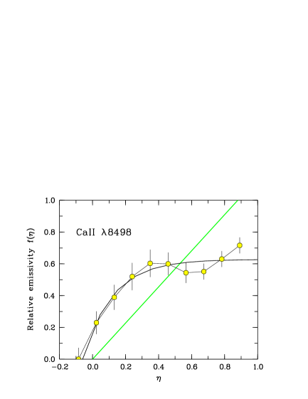
Figure 10: Variation of the flux in the CaII$\lambda 8498$ emissivity as a function of $\eta=\mathrm{cos}\,\vartheta$ for irradiation by a point source. The green line is for emission proportional to the energy influx, the black curve, for a simple analytical model that concentrates the emission closer to the terminator, and the open circles for the numerical tomographic model.

6 Model fits

Narrow emission lines have been detected in many CVs and have been used to determine binary parameters assuming an origin from the irradiated face of the secondary. We confirm this origin for EX Hya, but the interpretation of these lines is by no means straightforward. The centroid of the emission depends on the model parameters and minimum $\chi^{2}$ may occur for different values of the total mass $M$ depending on the choice of $f(\eta)$ and $c_{\mathrm{lim}}$. The situation differs if absorption and emission lines are considered together because then the model covers the entire range of radial velocities that occur over the surface of the secondary star. To obtain an internally consistent fit, we impose the side condition that the fit assumes minimum $\chi^{2}$ for the CaII lines and the NaI lines at the same $M$, by appropriately adjusting the parameters of the emission line model. All fit results presented in this paper comply with this condition.

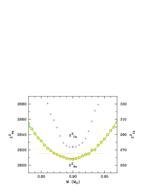
Figure 11: Result of the multiparameter fit for the numerical model of the CaII emissivities of Fig. 10. The NaI value $\chi^{2}_{\mathrm{Na}}$ (open circles) is shown as a function of total mass $M$ with the other parameters free, the CaII value $\chi^{2}_{\mathrm{Ca}}$ (+) is slaved to reach its minimum at the same value of $M$ (requiring $c_{\mathrm{lim}}=-0.085$). The green curve is a parabola fit and the dotted line indicates the 99% confidence level.

6.1 CaII$\lambda 8498$ emissivity

A representative set of emission models is shown in Fig. 10. The simple assumption of emission proportional to the incident energy flux, $f(\eta)\propto\eta$ (green line), utterly fails yielding profiles at quadrature that lack intensity at the higher velocities and require relatively more emission at small $\eta$. A one-parameter model of the form $f(\eta)\propto 1-\mathrm{exp}(-\alpha\eta)$ fairs much better. The best fit requires $\alpha=5.9$ and $c_{\mathrm{lim}}=-0.060$ (black solid line). The tomographic model with eight fitted emissivities $f_{\mathrm{m}}$ (Sect. 5) yields a slightly improved fit. The displayed model (open circles) is for an intermediate level of regularization with a Lagrange multiplier $A$ = 100 and requires $c_{\mathrm{lim}}=-0.085$. Lower and higher values of $A$ produce a more or less pronounced emission peak near $\eta\simeq 0.3$ and the error bars on the data points reflect the range $A$ = 0 to 1000. Despite the slightly negative values of $c_{\mathrm{lim}}$ for both models, the emission is practically limited to the illuminated part of the star if we consider that the finite extent of the source at the white dwarf (Siegel et al. 1989) alone accounts for a fuzziness of the terminator of about $2^{\circ}$ ($\Delta c_{\mathrm{lim}}=\pm 0.035$). Furthermore, the models lack the resolution to account for an abrupt drop of the emissivity at $\eta=0$. Hence, the slight extension of the emission beyond the geometric terminator is only marginally significant and we conclude that there is no compelling evidence for lateral energy transport in the atmosphere across the terminator. On the other hand, it is highly significant that the emission decreases much slower with decreasing $\eta$ than the incident energy flux. The observed increase in $f(\eta)/\eta$ as the terminator is approached is qualitatively expected from the calculations of König et al. (2006) for the hydrogen Lyman line emission from an irradiated (white dwarf) atmosphere. Realistic calculations are complex and need to consider the spectral energy distribution of the incident radiation and its degradation as the terminator is approached in a spherically extended irradiated atmosphere treated in 2-D or 3-D.

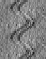
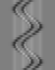
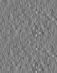
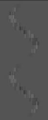
Figure 12: a–f.  Sections of Fig. 5 containing the NaI$\lambda 8183/8195$ doublet and the CaII$\lambda 8498$ emission line. The Paschen background has been subtracted in the latter. The three panels each (a–c and d–f) show the data (left, a, d), the model (center, b, e), and the residual fluxes (right, c, f). The displayed intensities are relative to the orbital mean, the zero level is shaded gray, lower and higher intensities appear darker and lighter, respectively. FeI$\lambda 8220.4$ appears as very faint emission line in panels a and c, rows 7 to 10. The gray scales in the NaI and CaII images differ.

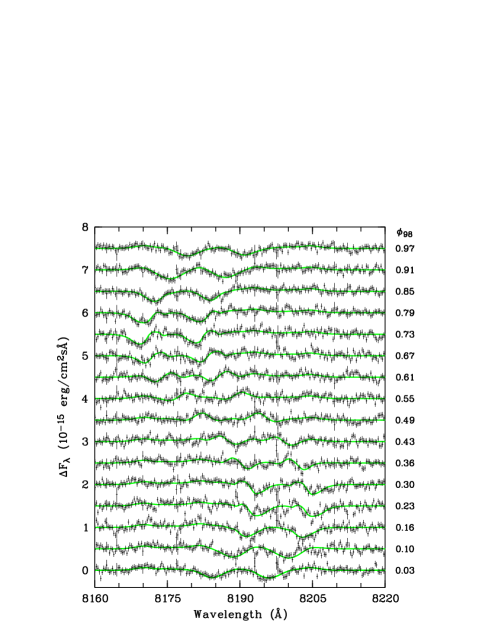
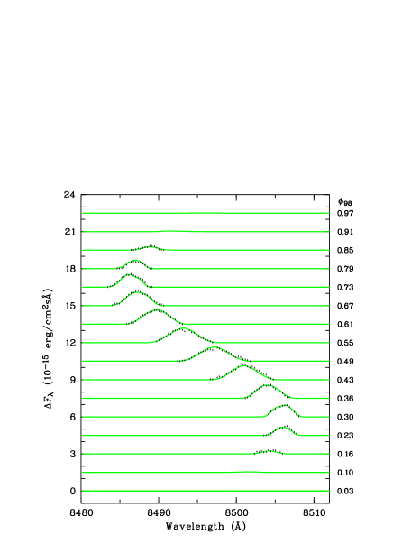
Figure 13: a,b.  Comparison of observed phase-resolved line profiles (data points) and best-fit model spectra (green curves) for the NaI$\lambda 8183/8195$ doublet (left, a) and the CaII$\lambda 8498$ emission line (right, b). The Paschen background has been subtracted in the latter.

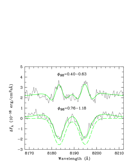
Figure 14: Observed (black) and fitted (green) line profiles of the NaI line for the illuminated (top) and dark side (bottom) of the secondary star. Same data as in Fig. 13 shifted into the respective rest system and co-added for two phase intervals (see Sect. 5.4). See text for further explanation.

6.2 Line profiles and quality of the fit

The high quality of the fit to the phase-resolved line profiles of the residual spectra (Sect. 3.3) is demonstrated in Figs. 12 and 13. Figures 12a and d show excerpts of Fig. 5 that cover the NaI$\lambda 8183/8195$ doublet and the CaII$\lambda 8498$ emission line, respectively, the model line profiles are shown in Figs. 12b and e, and the residuals between data and model in Figs. 12c and f. Figures 13a,b display a quantitative version of the same result. There is no background in the CaII line profiles since they have been extracted from the profiles of Fig. 5 by removal of the underlying Paschen background. The enhanced emission at the extremal velocities of the NaI doublet in Fig. 12b are a result of the subtraction of the orbital mean spectrum from the data and the model as described in Sect. 3.3. The sodium doublet is fitted between 8160.5 and 8214.5Å and contributes 2880 data points in the 16 phase intervals, while the CaII data set contains 250 non-zero data points. The best fit has $\chi^{2}_{\mathrm{Na}}=2608$ and $\chi^{2}_{\mathrm{Ca}}=274$, or a total  $\chi^{2}=2882$ for 3116 d.o.f. With a reduced $\chi^{2}_{\nu}$= 0.925, the fit is clearly good. The NaI part benefits from the inclusion of pressure broadening (Fig. 13a), while the CaII profiles (Fig. 13b) are well matched without any additional broadening beyond radial velocity smearing. The humps that appear on the low-velocity slopes of the CaII profiles at $\phi_{98}$= 0.30 and 0.73 are responsible for the enhanced emissivity near $\eta=0.3$ in Fig. 10. Some variability in the individual CaII profiles can not be matched by the adjustment of parameters and may indicate temporal fluctuations of the line emission.

Figure 14 shows the spectra observed from the illuminated and the dark side of the star shifted into their respective rest systems. The emission line profile (top) displays dips flanking the emission peaks that represent residues of the incomplete fill-up of the underlying absorption components. The dips support our choice of model for the composite NaI line profiles (Sect. 5.2). The observed absorption line profile (bottom) is accompanied by model spectra with and without the orbital mean subtracted (solid and dashed green curves, respectively). They demonstrate that the subtracted model retains about 90% of the signal, provided the spectral structure is restricted to a narrow wavelength range. The result justifies our use of the mean observed spectrum as a template for the telluric line correction.

Finally, Fig. 7 compares the integrated observed and modeled CaII emission line fluxes of Fig. 13b as a functions of orbital phase (upper panel, black histogram and green curve). The observed slight asymmetry of the light curve is modeled by assuming the ’hot spot’ as a second source of irradiation. Some other physical effect can not be excluded.

6.3 System parameters

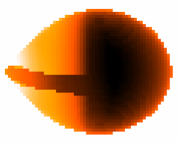
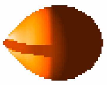
Figure 15: a,b.  Tomographic images of the secondary star of EX Hya seen at $\phi_{98}=0.75$ and $i=77.8^{\circ}$ for the numerical model of the emissivities of Fig. 10. (a) Left: NaI$\lambda 8183/8195$ absorption/emission, (b) right: CaII$\lambda 8498$ emission. The $x^{\prime}-z^{\prime}$ plane is perpendicular to the line of sight and coordinates are relative to the binary separation $a$ with the origin in the white dwarf. The geometric terminator for illumination by a point source at the white dwarf is indicated by the dashed line. The intensity scales differ for both images. In the left hand panel, black is absorption, white emission, and the red rim represents zero intensity, while the dark side of the star in the right panel denotes zero line flux that increases over red to white. Faint emission in the disk shadow and beyond the terminator is due to irradiation by the ’hot spot’.

Figure 11 shows the variation of the $\chi^{2}_{\mathrm{Na}}$ vs. total mass $M$ for the NaI lines with $\chi^{2}_{\mathrm{Ca}}$ for the CaII emission slaved to assume a minimum at the same $M$ by appropriate choice of the parameters of the numerical emission model. There is a well defined $\chi^{2}$ minimum at a total system mass $M=0.898$ M_⊙, with an error of 0.026 M_⊙ at the 99% confidence level (dotted line). This result is obtained with a radial velocity amplitude of the white dwarf of 59 km s^-1 (Belle et al. 2003; Hoogerwerf et al. 2004) and a system inclination of $77.8^{\circ}$. The uncertainties in $K_{1}$ and $i$ of about 3 km s^-1 and $0.4^{\circ}$ add $\pm 0.016$ M_⊙ and $\pm 0.005$ M_⊙ to the error budget of $M$, respectively. Adding the errors quadratically, our measured system mass is $M=0.898\pm 0.031$ M_⊙. The remaining fit parameters are summarized in Tab. 4.

The slightly mass-dependent inclination $i=(77.8\pm 0.4)^{\circ}$ is determined from the FWHM of the X-ray eclipse of 155 s (Mukai et al. 1998; Hoogerwerf et al. 2005) on the assumption that only the lower pole of the white dwarf is eclipsed and is responsible for the partial character of the X-ray eclipse (Beuermann & Osborne 1988; Beuermann et al. 2003). Some variants of the model (Hellier et al. 1987; Rosen et al. 1988, 1991) may yield a slightly different value of $i$ and we note that a $\pm 1^{\circ}$ change in $i$ causes a shift of $\mp 0.012$ M_⊙ in $M$.

The velocity amplitude $K_{2}$ of the secondary star is a derived quantity and equals $K_{2}=(2\pi\mathrm{G}M/P)^{1/3}\mathrm{sin}\,i-K_{1}=432.4\pm 4.8$ km s^-1. The mass ratio is also a derived quantity and given by $q=K_{1}/K_{2}=0.1365\pm 0.0071$. The error in $K_{2}$ is almost entirely due to the noise in the line profiles, while the error in $q$ reflects mostly the uncertainty in $K_{1}$. The masses of primary and secondary are $M_{1}=0.790\pm 0.026$ M_⊙ and $M_{2}=0.108\pm 0.008$ M_⊙, respectively. The mean Roche lobe radius of the secondary star is $R_{2}=0.1516\pm 0.0034$ R_⊙. Our direct fit to the line profiles eliminates all problems associated with the determination of radial velocities from the complex line profiles as far as possible. Our result for $K_{2}$ significantly exceeds the value of $360\pm 35$ kms reported by Vande Putte et al. (2003), on which most recent published $M_{1}$ values were based. The system velocity obtained from the fit is $\gamma=-58.2\pm 1.0$ km s^-1 in agreement with the result obtained in Sect. 4.2 from the radial velocity curves.

6.4 Roche tomography

Roche tomography subjects the emission of all surface elements to some type of regularization and works best if the binary parameters are known (Watson & Dhillon 2004). Since the determination of these parameters is our main goal, our tomographic approach involves the following simplifications: (i) there is no freedom in the contributions of the individual surface elements to the NaI absorption line profiles (Sect. 5.3); and (ii) the contributions to the emission line profiles depend only on the angle of incidence $\vartheta$ of the irradiation, with shadowing by the accretion disk superimposed (Sect. 5.4). However, as discussed above, there is freedom in the dependence of the emission line flux on the incident energy flux, in the extent to which the emission extends into the ’dark’ side of the star, and in the angular distribution of the emission line intensity that emerges from a given surface element (Sect. 5.4). The fact that the model fits the data with a reduced $\chi^{2}_{\nu}$=0.92 indicates that any added freedom in the tomography can not be expected to improve the fit. Such an approach would need data of much better statistical significance.

Figure 15 shows the images of the secondary star derived from our restricted tomography as seen at orbital phase 0.75 and an inclination of $77.8^{\circ}$. The left panel depicts the NaI image and the right panel the CaII image. The pictures are based on the numerical model of the emission line fluxes of Fig. 10. The principal features are the clear distinction between dark and irradiated hemispheres of the secondary star and the dark lane representing the shadow cast by the accretion disk. The geometric terminator for illumination by a point source at the position of the white dwarf is indicated by the dashed line. Emission is seen to cease rather abruptly within a few degrees of the terminator, except for the faint emission produced by the ’hot spot’ that extends beyond the terminator and fills in the disk shadow. In the NaI image, the effect of limb (and gravity) darkening is visible as a reduced absorption line flux as the limb is approached. The shadow of the accretion disk takes away emission very close to the L₁ point, but otherwise has little effect on the relative distribution of the emission.

7 Discussion

The main result of our high-resolution spectrophotometric study is the discovery of narrow absorption and emission lines from the photosphere and chromosphere of the illuminated secondary star in EX Hya. We present a novel method for the kinematic analysis that involves a direct fit of a model of the emitting Roche-lobe filling secondary star to the observed absorption and emission line profiles. A key quantity is the linear size of the Roche lobe between its back and the L₁-point (Sect. 4.3), which we determine from the combined fit of the synthesized line profiles to the absorption and the emission line data. Combined with the previously measured radial velocity amplitude $K_{1}$ of the white dwarf (Belle et al. 2003; Hoogerwerf et al. 2004), this line synthesis approach allows us to determine accurate masses of the binary components.

Table 5: Parameters of the secondary star in EX Hya compared with those of Gl551 (Proxima Cen).

Parameter	EX Hya B	Gl5511
Spectral type	dM$5.5\pm 0.5$	dM5.5
Temperature $T_{\mathrm{eff}}$ (K)		$3042\pm 117$
Distance $d$ (pc)	$64.5\pm 1.2$	$1.295\pm 0.007$
$K$ (mag)	$12.89\pm 0.11$	4.36
$M_{\mathrm{K}}$ (mag)	$8.83\pm 0.12$	$8.80\pm 0.02$
Mass $M$ (M⊙)	$0.108\pm 0.008$	$0.123\pm 0.006$
Radius $R$ (R⊙)	$0.1516\pm 0.0034$	$0.145\pm 0.011$
Velocity amplitude $K_{2}$ (km s-1)	$432.4\pm 4.8$
Systemic velocity $\gamma$ (km s-1)	$-58.2\pm 1.0$

¹⁾ From Ségransan et al. (2003)

7.1 The secondary star

Our fit yields a secondary mass $M_{2}=0.108\pm 0.008$ M_⊙ and a mean Roche radius $R_{2}=0.1516$ R_⊙=$1.05\times 10^{10}$ cm, which place the star much closer to the main sequence than the former estimate of 0.078 M_⊙ (e.g., Beuermann et al. 2003). The absolute $K$-band magnitude of EX Hya B is $M_{\mathrm{K}}=8.83\pm 0.12$ in perfect agreement with the spectral classification dM$5.5\pm 0.5$. The derived parameters of EX Hya B are summarized in Tab. 5, with the data of the nearby dM5.5 star Gl551 that has an interferometrically measured radius (Ségransan et al. 2003) added for comparison. The radius of an 0.108 M_⊙ model star of solar composition is $0.925\times 10^{10}$ cm (Baraffe et al. 1998) and rises to $0.98\times 10^{10}$ cm if rotational deformation is accounted for (Renvoizé et al. 2002). These models apply to stars without spots, while spotted stars tend to have somewhat larger radii. Just how much this effect influences the radii of the secondary stars in CVs is not known (see Beuermann et al. 2006 and references therein). The calibration of the radii of field stars vs. $M_{\mathrm{K}}$ (Beuermann et al. 1999, Eq. 7)  yields $R=0.1514$ R_⊙ for $M_{\mathrm{K}}=8.83$, confirming that EX Hya B is essentially a main sequence star, but differs from a field star of the same absolute magnitude by being deformed and irradiated.

7.2 The white dwarf

Previous estimates of the masses of the two stellar components in EX Hya relied on the uncertain velocity amplitude of the secondary star of Vande Putte et al. (2003), $K_{2}=360\pm 35$ km s^-1. Our result, $K_{2}=432.4\pm 4.8$ km s^-1, is 2.1$\sigma$ from Vande Putte’s result and yields a much more accurate kinematic solution. The primary mass $M_{1}=0.790\pm 0.026$ M_⊙ supersedes the value of $M_{1}\simeq 0.46$ M_⊙ quoted in most recent studies on EX Hya (e.g. Beuermann et al. 2003; Vande Putte et al. 2003; Hoogerwerf et al. 2004, 2005; Mhlahlo et al. 2006) . The new mass is close to the mean for short-period CVs, $\langle M\rangle\simeq 0.8$ M_⊙, and confirms the early result $M_{1}=0.78\pm 0.17$ M_⊙ of Hellier et al. (1987). Given the larger primary mass, one can re-estimate the mass transfer rate following the analysis of Beuermann et al. (2003, see also Ritter (1985)). From their Fig. 1, $\dot{M_{1}}$ is seen to drop with increasing $M_{1}$ and reach about the value expected from gravitational radiation as the sole momentum transfer process for $M_{1}=0.79$ M_⊙.

The radius of a white dwarf of $0.790\pm 0.026$ M_⊙ with an intrinsic effective temperature of about 15000 K is $R_{1}=(7.35\pm 0.23)\times 10^{8}$ cm based on models with a thick hydrogen envelope (Wood 1995). The mean temperature of the white dwarf in EX Hya determined from the HST FOS spectrum is 25000 K (Eisenbart et al. 2002), but that temperature is dominated by the heated polar caps responsible for the pronounced spin modulation seen in X-rays and in the UV and the temperature of the underlying white dwarf is likely to be lower, roughly as noted above. With the quoted radius, the gravitational redshift at the surface of the white dwarf is $\upsilon_{\mathrm{grav}}=47.6\pm 3.1$ km s^-1. The predicted apparent systemic velocity of the white dwarf then is $\gamma+\upsilon_{\mathrm{grav}}=-10.6\pm 4.1$ km s^-1. The velocity derived from the X-ray emission lines that originate close to the white dwarf surface is $\gamma=-2.8\pm 2.3$ km s^-1 (Hoogerwerf et al. 2004), where the error is the statistical one and the systematic error is larger (C. Mauche, private communication). While the interpretation of these numbers in terms of a gravitational redshift measurement may be premature, it is clear that an independent measurement of the white dwarf mass becomes feasible with a more secure value of the apparent systemic velocity of the white dwarf.