Chandra HETG Spectra of SN 1987A at 20 years

Abstract

We have undertaken deep, high-resolution observations of SN 1987A at $\approx$ 20 years after its explosion with the Chandra HETG and LETG spectrometers. Here we present the HETG X-ray spectra of SN 1987A having unprecedented spectral resolution and signal-to-noise in the 6 Å to 20 Å bandpass, which includes the H-like and He-like lines of Si, Mg, Ne, as well as O VIII lines and bright Fe XVII lines. In joint analysis with LETG data, we find that there has been a significant decrease from 2004 to 2007 in the average temperature of the highest temperature component of the shocked-plasma emission. Model fitting of the profiles of individual HETG lines yields bulk kinematic velocities of the higher-Z ions, Mg and Si, that are significantly lower than those inferred from the LETG 2004 observations.

1 Introduction

Twenty years after outburst, SN 1987A (catalog SN 1987A) is now well into its supernova remnant phase, such that its observed luminosity is dominated by the impact of the supernova debris with its circumstellar medium (McCray, 2007), the X-ray luminosity has brightened by a factor $\sim 25$ since first observed by Chandra in 1999 (Aschenbach, 2007), and is currently brightening at a rate $\sim 40\%$ per year (Park et al., 2007). The X-ray image seen by Chandra is an expanding elliptical ring; its brightness distribution is correlated with the rapidly brightening optical hotspots on the inner circumstellar ring seen with the Hubble Space Telescope. Assuming that the X-ray emission is a circle inclined at $45^{\circ}$ (north side toward Earth), its inferred radial velocity is currently $1412\pm 354$ km s^-1(Park et al., 2007).

Michael et al. (2002) reported the first observation of the X-ray spectrum taken with the High Energy Transmission Grating (HETG) on Chandra in October 1999. That observation, of 116 ks duration, showed that the X-rays had an emission line spectrum characteristic of shocked gas. But that spectrum had insufficient counting statistics (e.g., only 19 counts in O VIII L$\alpha$) to provide reliable line profiles or accurate line ratios. As the X-ray luminosity of SN 1987A has continued to increase, it has become possible to measure emission line ratios and profiles with sufficient accuracy to permit quantitative interpretation of the shock interaction responsible for the X-ray emission. Dispersed X-ray spectra of SN 1987A have been obtained with the Reflection Grating Spectrometer on XMM-Newton in May 2003 (Haberl et al., 2006) and again in January 2007 (Heng et al., 2008), and with the Low Energy Transmission Grating (LETG) on Chandra (289 ks duration) in August-September 2004 (Zhekov et al. (2005, 2006) – hereafter Z05, Z06).

With angular resolution FWHM $\sim 0.7\arcsec$, Chandra can resolve the circumstellar ring ($1.2\arcsec\times 1.6\arcsec$) of SN 1987A. This angular resolution is vital for interpreting the linewidths seen in the dispersed X-ray spectra, which are a convolution of the spatial structure of the X-ray image and the kinematics of the X-ray emitting gas. As Z05 have described, one can separate these contributions by comparing the $m=+1$ and $m=-1$ orders of the dispersed spectrum: with the dispersion axis along the N-S direction, the images of the ring in spectral orders dispersed to the north will be “compressed”, and those to the south will be “stretched” (Z05).

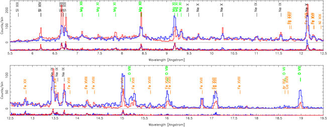
Figure 1: HETG SN 1987A Spectra. Observed counts spectra from all of the observations, totaling 360 ks, are shown; the MEG minus (blue) and plus (red) order spectra are plotted along with offset HEG spectra (same color coding.) The MEG[HEG] bin size is 0.020[0.010] Å, equivalent to $\approx$ 1″ in spatial extent. The wavelengths of expected bright lines are indicated as well.

We have obtained new Chandra spectra of SN 1987A, in March 2007 with the HETG (catalog ADS/Sa.CXO#Obs/8523) (HETG’07) and in September 2007 with the LETG (LETG’07). In this Letter we focus on the HETG results, which have substantially greater counting statistics and better spectral resolution than the LETG’04 spectra (Z05), and which lead to a significant clarification of Z05’s inferred relationship between bulk motion and ion species. Moreover, we see significant evolution of the thermal structure of the interaction since the 2004 observations. Preliminary analysis of the LETG’07 data confirms that this evolution is not an effect of the spectrometer being used. In a subsequent paper, we will provide a more detailed analysis and interpretation of the combined HETG and LETG observations.

2 Observations and Data Reduction

The HETG’07 observations were carried out as part of the GTO program in spring 2007 near a roll angle of 270 degrees, imaging the “stretched” orders on the ACIS-S1 BI chip (which has the best low-energy sensitivity.) The data consist of 14 observations with roll angles from $270^{\circ}$ to $238^{\circ}$ during SN day 7321 to 7358, for a total live time of 354.9 ks. We used the standard CIAO tools and HETG extraction procedures to process the data sets. The tgdetect routine located the zeroth order near the “dark center” of each event image to better than 0.1 arc second. The nominally extracted first-order spectra contain the following numbers of counts: 15.2 k (MEG-1), 14.0 k (MEG+1), 5.8 k (HEG-1) and 4.7 k (HEG+1). In Figure 1 we display all four first-order counts spectra in the high S/N range, 5.5 to 19.5 Å. The higher resolution and lower effective area of HEG compared to MEG spectra are evident, e.g., at the Ne triplet $\sim 13.5$Å; we also display close-ups of the beautifully resolved He-like triplets for Si and Mg in Fig. 2.

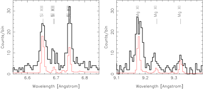
Figure 2: Si and Mg triplets resolved. The Si (left) and Mg (right) triplets are plotted as observed in the plus (“compressed”) order of the HEG. The data are shown by the solid black histogram and an arbitrarily-scaled point-source version of the 2-shock model (no spatial-velocity effects) is shown in red to suggest the relative similarity of the data and model G-ratios ( (f+i)/r ).

3 Shock Emission Measure Distribution

Following the analysis procedures of Z06, we performed global fits to the data with two models: (i) a simple 2-shock model and (ii) a distribution of shock emission measures model, “$EM(T)$”. In the latter model, the basic vectors characterizing the spectral distribution are plane-parallel shocks characterized by their mean post-shock temperature and a related ionization timescale.

We simultaneously fit the six background-subtracted $\pm 1^{\rm st}$-order spectra from the LETG’04, HETG’07 (MEG) and LETG’07 data sets, rebinning all spectra to have a minimum of 30 counts per bin. We assumed common values among the data sets for $N_{\rm H}$, the interstellar absorption column density, as well as the chemical composition of the hot, shocked plasma. Specifically, we fixed the abundances  of H, He, C, Ar, Ca and Ni to the values given in Z06, and we allowed the abundances of N, O, Ne, Mg, Si, S and Fe to vary in our fits.

Figure 3: Emission measure distribution versus shock temperature. $EM(T)$ as derived with 25 points logarithmically spaced in the ($0.1-4$ keV) post-shock temperature range. A disproportionate growth of $EM(T)$ is seen in the mid-T range, $\sim 1.4$ keV. For reference, the arrows indicate the post-shock temperatures of the simple 2-shock model fits given in the text; low (high) temperature components are plotted from the lower (upper) x-axis.

In principle some evolution of the chemical composition might take place as a result of evaporation of dust grains in the shocked gas. However, as Dwek & Arendt (2007) have shown, the dust grains in SN 1987A appear to have such low abundance of that they cannot contribute substantially to the gas phase abundance of heavy elements. Likewise we are assuming uniformity of composition throughout the ring. These assumptions of stationary and uniform abundances in time and space are taken as a starting point for these analyses.

For the 2-shock model joint fits, the derived values and 90 % confidence limits (in brackets) for the absorption column density ($N_{\rm H}=1.30$ [1.18–1.46] $\times 10^{21}$) and elemental abundances (N=0.56 [0.50–0.65], O=0.081 [0.074–0.092], Ne=0.29 [0.27–0.31], Mg=0.28 [0.26–0.29], Si=0.33 [0.32–0.35], S=0.30 [0.24–0.36] and Fe=0.195 [0.189–0.206]) are all within or very near the 90 % limits presented in Z06. The values of $kT_{\rm low}$ (keV) are very similar for all three data sets: 0.53 [0.50–0.55], 0.56 [0.53–0.59], and 0.54 [0.53–0.56] for the LETG’04, HETG’07, and LETG’07 data, respectively. In contrast, the $kT_{\rm high}$ (keV) values indicate a general evolution toward lower values across these same data sets: 2.7 [2.5–3.0], 2.4 [1.9–2.7], and 1.9 [1.8–2.0] . This result confirms a similar trend seen in the “$kT({\rm hard)}$” values derived from ACIS monitoring of SN 1987A (Park et al., 2006, 2007).

The decrease in $kT_{\rm high}$ is echoed by an evolution of the shock emission measure distributions, $EM(T)$, that we derive from global fits to the three data sets, Figure 3. First, note that the fits to the 2007 LETG and MEG data are very similar. The value of $EM(T)$ derived from LETG’07 data is slightly greater than that derived from the 2007 MEG because the source brightened by a factor $\approx 1.17$ between Mar-Apr 2007 and Sep 2007. We see more substantial evolution in $EM(T)$ from 2004 to 2007. Like the 2004 $EM(T)$, the 2007 $EM(T)$ is bimodal, having a low temperature peak at 0.55 keV and a high temperature peak at $\sim 2$ keV. During the interval Sep 2004 to Mar-Apr 2007, the shape of the low temperature peak did not change, but the total emission brightened by a factor $\sim 2.47$, corresponding to a doubling timescale of approximately two years. At higher temperatures the shape of the $EM(T)$ appears to have evolved substantially in addition to the increased amplitude. We see substantial “filling in” of emission measure in the intermediate $T$ range, 1.0–2.5 keV, and a decrease in the highest temperature bin ($>3$ keV). Further analysis will be needed to quantify the significance of these apparent changes.

4 Line Profiles: Expanding Ring Model

We fit the observed line profiles with a simple model incorporating the basic spatial-kinematic properties of SN 1987A’s geometry, enabling us to infer an average expansion velocity, $v_{\rm ring}$, for each emission line. The geometric model is a torus with specified inner (1.55″) and outer (1.7″) diameters with its axis oriented in space ($42.8^{\circ}$ S and $10^{\circ}$ E from the line-of-sight.) The torus has a non-uniform azimuthal intensity distribution determined from the observed zeroth-order imaging data. Emission at each location on the ring is Doppler shifted by the combination of the component of radial expansion at that point along the line of sight, the overall systemic velocity, and an additional Gaussian Doppler broadening term, $\Delta v_{\rm los}$, along the line-of-sight.

We implemented the above as a custom model  in ISIS (Houck, 2002). We use a Monte Carlo scheme to evaluate the line profile for the particular model parameters, also taking into account the properties of the specific data set (the grating, order, and observation roll angle.) We sum one (or two in the case of blended lines) of these “ring model” line shapes with the nominal 2-shock model in which the abundance of the element being fit is set to zero. We tie the 2-shock norms together in the appropriate ratio and allow them to vary in the line fitting. In this way, we have an accurate continuum shape and also make some allowance for contaminating lines, e.g., Fe lines in the Ne triplet region.

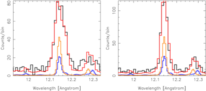
Figure 4: Example of the spatial-spectral model fit. The MEG minus (left) and plus (right) order data (black) for the Ne X line are show with the best-fit model overplotted (red.) For reference, the low and high $T$ components of the 2-shock model are shown at point-source resolution (orange and blue, respectively.)

We fit the data from the first 319 ks (excluding the last observation taken at a roll angle $25^{\circ}$ from the average) with this model in a limited wavelength region around each line. We used all four HEG/MEG $\pm 1$-order spectra except in the long wavelength range ($>16$Å) where we excluded one or both of the HEG spectra from the fits because of a lack of counts. Figure 4 illustrates the fit to the Ne X line in the MEG $\pm 1$-order spectra. We tabulate the results for the bright lines in the spectrum in Table 1 and display their ring expansion velocities in Fig. 5. The best-fit values for the additional Doppler broadening parameter, $\Delta v_{\rm los}$, (not tabulated) are in the 300–700 km s^-1 FWHM range.

Table 1: Fit Parameters for the Non-uniform Ring Model.

Ion	$\lambda_{\rm t}$	$\lambda_{\rm fit}$$\,(1\sigma)$	$v_{\rm ring}\tablenotemark{\,c}\,\pm 1\,\sigma$	Flux
Si XIV L$\alpha$	6.183	6.181(1)	456., 322–641	4.6 ${{\pm 10\%}}$
Si XIII r ()	6.648	6.650(1)	450., 370–574	14.5 ${{\pm\ 5\%}}$
& Si XIII i	6.687	6.691(5)	”	3.4 ${{\pm 16\%}}$
Si XIII f	6.740	6.738(1)	203.,    0–360	6.3 ${{\pm\ 9\%}}$
Mg XII L$\alpha$	8.422	8.421(1)	380., 302–471	11.0 ${{\pm\ 6\%}}$
Mg XI r ()	9.169	9.170(1)	303., 230–375	22.3 ${{\pm\ 5\%}}$
& Mg XI i	9.230	9.228(3)	”	5.3 ${{\pm 15\%}}$
Mg XI f	9.314	9.315(2)	357., 230–516	7.0 ${{\pm 12\%}}$
Ne X L$\beta$	10.239	10.241(2)	396., 267–533	10.8 ${{\pm 10\%}}$
Ne IX 3-1	11.544	11.545(2)	32.,    0–194	11.0 ${{\pm 12\%}}$
Ne X L$\alpha$	12.135	12.134(1)	375., 309–439	72.0 ${{\pm\ 4\%}}$
Ne IX r ()	13.447	13.448(1)	253., 146–323	62.0 ${{\pm\ 6\%}}$
& Ne IX i	13.552	13.552(3)	”	16.0 ${{\pm 16\%}}$
Ne IX f	13.699	13.698(1)	189., 121–282	36.7 ${{\pm\ 9\%}}$
Fe XVII	15.014	15.014(1)	361., 295–411	75.0 ${{\pm\ 6\%}}$
O VIII L$\beta$	16.006	16.006(3)	539., 434–648	42.6 ${{\pm 11\%}}$
Fe XVII	16.780	16.775(3)	260., 170–344	33.5 ${{\pm 13\%}}$
Fe XVII ()	17.051	17.051(4)	123 ,  60–304	27.4 ${{\pm 17\%}}$
& Fe XVII	17.096	17.094(3)	”	41.7 ${{\pm 13\%}}$
O VIII L$\alpha$	18.970	18.970(3)	172., 70–272	103. ${{\pm 10\%}}$
O VII r	21.602	21.60(1)	259.,    0–431	28. ${{\pm 40\%}}$
O VII f	22.098	22.01(1)	208.,    0–350	33. ${{\pm 40\%}}$
N VII L$\alpha$	24.782	24.77(1)	189.,  45–333	75. ${{\pm 22\%}}$

The bulk velocities measured with the HETG’07 data (the diamond symbols in Figure 5) are significantly lower, by a factor of 2 at Si and Mg, than those inferred from the “stratified” model that was employed to fit the LETG’04 FWHM data (dashed line). The new HETG data are, however, in good agreement with the constant velocity model of Z05 (dotted line). Note that there is the hint of a much reduced “stratified” trend: expansion velocities tending to increase toward shorter wavelengths.

Figure 5: “Ring” velocities versus wavelength. The HETG-measured radial velocities and their one sigma ranges are plotted against the line wavelength. For comparison the “stratified” (dashed) and “constant” (dotted) radial velocities from Z05 are overplotted. The stratified model is clearly excluded by the new HETG data.

5 Discussion

The most striking result that we find from the HETG data is the relatively low bulk radial velocity of the shocked gas in the ring. In a simple model consisting of a plane-parallel strong shock entering a stationary gas, the bulk velocity of the shocked thermal plasma should be given by $v_{\rm psh}=3/4\,v_{\rm sh}$, and the post-shock mean plasma temperature should be given by $kT=1.4(v_{\rm sh}/1000~{}\mathrm{km\,s^{-1}})^{2}$ keV (for mean molecular weight $\mu=0.72$ based on our abundances, see also Z06). Then, setting $v_{\rm psh}=v_{\rm ring}$, we would expect post-shock temperatures in the range $kT\sim 0.1-0.6$ keV for the observed range $v_{\rm ring}\sim 200-500$ km s^-1 (Fig. 5). This temperature range is much lower than the range $0.3-3$ keV inferred from the spectral modeling of the emitting gas. Clearly, such a simple shock model is inadequate to describe the actual system.

The range of broadening, $\Delta v_{\rm los}$, used in the fits to the line profile, 300-700 km s^-1 FWHM, generally exceeds the expected thermal line-of-sight contribution, given by $\Delta v_{\rm therm}=163\,\sqrt{E_{\rm keV}/(A/20)}$ km s^-1 FWHM where $E_{\rm keV}=kT_{\rm i}$ is the ion temperature in keV and $A$ is the atomic weight of the ion. For $E_{\rm keV}=0.4-3$ the range of thermal Doppler widths (FWHM) is: 115–315 (O); 87–237 (Si); and 61–170 (Fe).

The fact that the X-ray image is correlated with the optical hotspots leads us to a picture in which the blast wave ahead of the supernova debris is overtaking dense clumps of circumstellar gas associated with the hotspots. Since these hotspots are unresolved, we can only guess at their geometry and density distribution. But it would be reasonable to expect that the X-ray emitting gas spans a range of densities and has complex morphology.

If a blast wave runs into a clump of high density at normal incidence, the transmitted shock might be too slow to emit X-rays but the shock encountering the clump would be reflected. The reflected shock would leave behind twice-shocked gas having nearly stationary bulk velocity but further elevated temperature. As more and more of the X-ray emission comes from gas behind such reflected shocks, we would expect that the fraction of the X-ray emission measure at higher temperatures would increase, while the average bulk velocity would decrease. And that is what we see.

In addition, much of the X-ray emission probably comes from shocks resulting from the blast wave encountering dense clumps at oblique incidence, in which case the shocked gas would have significant velocity components parallel to the shock surface. We suspect that the complex hydrodynamics resulting from both transmitted and reflected shocks encountering the circumstellar ring at normal and oblique incidence is responsible for the Doppler broadening seen in the line profiles.

As Table 1 shows, the radial expansion velocity of the ring inferred from the X-ray line profiles ranges from $\sim 200-450$ km s^-1, much less than the value $1412\,\pm 354$ km s^-1 inferred from the expansion of the X-ray image (Park et al., 2007). The expansion of the X-ray image tells us the location of the centroid of the X-ray emitting ring, which is determined by the average radius of the relatively dense ($n>10^{4}$ cm^-3) shocked gas. We believe that these dense clumps or fingers are being overtaken by a blast wave that is propagating at radial velocities $v>2000$ km s^-1 through gas of relatively low density ($n<10^{2}$ cm^-3), which does not contribute substantially to the observed X-ray emission. On the other hand, the velocities seen in the X-ray emission line profiles represent the actual kinematic velocities of the shocked gas surrounding the dense clumps, which are much less than the velocity of the blast wave.

There is much more that can be done with this data set – in particular looking at the full 2D distribution of the dispersed events instead of just their 1D projection. Especially in the “stretched” MEG-minus order, one may be able to measure spatially-resolved line ratios. Given the complexity of the SN 1987A system, such spatial analysis may identify emission from other geometric components of the system.

References

- Aschenbach (2007) Aschenbach, B. 2007, AIP Conf. Proc. 937, see McCray (2007), 33.
- Dwek & Arendt (2007) Dwek, E., & Arendt, R. G. 2007, AIP Conf. Proc. 937, see McCray (2007), 58.
- Haberl et al. (2006) Haberl, F., Geppert, U., Aschenbach, B., & Hasinger, G. 2006, A& A, 460, 811.
- Heng et al. (2008) Heng, K., Haberl, F., Aschenbach, B., & Hasinger, G. 2008, ApJ, in press.
- Houck (2002) Houck, J. C. 2002, High Resolution X-ray Spectroscopy with XMM-Newton and Chandra, 2002hrxs.confE..17H
- Huenemoerder et al. (2006) Huenemoerder, D. P., Testa, P., & Buzasi, D. L. 2006, ApJ, 650, 1119
- McCray (2007) McCray, R. 2007, in AIP Conf. Proc. 937, Supernova 1987A: 20 Years After. Supernovae and Gamma-Ray Bursts, ed. S. Immler, K. W. Weiler, & R. McCray (New York, AIP), 3.
- Michael et al. (2002) Michael, E., et al. 2002, ApJ, 574, 166
- Park et al. (2006) Park, S., Zhekov, S. A., Burrows, D. N., Garmire, G. P., Racusin, J. L., & McCray, R. 2006, ApJ, 646, 1001
- Park et al. (2007) Park, S., Burrows, D. N., Garmire, G. P., McCray, R., Racusin, J. L., & Zhekov, S. A. 2007, AIP Conf. Proc. 937, see McCray (2007), 43.
- Zhekov et al. (2005) Zhekov, S. A., McCray, R., Borkowski, K. J., Burrows, D. N., & Park, S. 2005, ApJ, 628, L127 (aka Z05)
- Zhekov et al. (2006) Zhekov, S. A., McCray, R., Borkowski, K. J., Burrows, D. N., & Park, S. 2006, ApJ, 645, 293 (aka Z06)