Properties of Consensus Methods for Inferring Species Trees from Gene Trees

James H. Degnan^1∗ Michael DeGiorgio², David Bryant³, and Noah A. Rosenberg^1,2

¹Department of Human Genetics, 1241 E. Catherine Street, University of Michigan, Ann Arbor 48109-0618, USA
^∗Corresponding author, E-mail: jamdeg@gmail.com
²Center for Computational Medicine and Biology, 2017 Palmer Commons, 100 Washtenaw Avenue, University of Michigan, Ann Arbor, 48109-2218 USA
³Department of Mathematics, University of Auckland, Private Bag 29019, Auckland, New Zealand

Abstract

Consensus methods provide a useful strategy for combining information from a collection of gene trees. An important application of consensus methods is to combine gene trees to estimate a species tree. To investigate the theoretical properties of consensus trees that would be obtained from large numbers of loci evolving according to a basic evolutionary model, we construct consensus trees from independent gene trees that occur in proportion to gene tree probabilities derived from coalescent theory. We consider majority-rule, rooted triple ($R^{*}$), and greedy consensus trees constructed from known gene trees, both in the asymptotic case as numbers of gene trees approach infinity and for finite numbers of genes. Our results show that for some combinations of species tree branch lengths, increasing the number of independent loci can make the majority-rule consensus tree more likely to be at least partially unresolved and the greedy consensus tree less likely to match the species tree. However, the probability that the $R^{*}$ consensus tree has the species tree topology approaches 1 as the number of gene trees approaches infinity. Although the greedy consensus algorithm can be the quickest to converge on the correct species tree when increasing the number of gene trees, it can also be positively misleading. The majority-rule consensus tree is not a misleading estimator of the species tree topology, and the $R^{*}$ consensus tree is a statistically consistent estimator of the species tree topology. Our results therefore suggest a method for using multiple loci to infer the species tree topology, even when it is discordant with the most likely gene tree.

The goal of many phylogenetic and phylogeographic studies is not the estimation of the individual gene trees, but rather the estimation of the species-level phylogeny or population history (Felsenstein, 1988; Takahata, 1989; Maddison, 1997; Nei and Kumar, 2000). Among methods that have been used to estimate species trees from data on multiple loci, a popular approach has been to make use of sequences concatenated across the loci. In essence, this approach assumes that all loci have the same gene tree, whose estimate is also used as the estimated species tree. Because gene trees vary both locally and across broad regions of organismal genomes (Chen and Li, 2001; Pollard et al., 2006; Hobolth et al., 2007), sequence data from multiple genes are expected to be the result of heterogeneous processes. Multilocus data can be regarded as mixtures generated from different branch lengths and mutation rates on gene trees as well as from different gene tree topologies that may arise from sources such as incomplete lineage sorting or hybridization.

As a result of these various sources of heterogeneity, concatenation can perform poorly when sequences are analyzed as if they come from a single model. Inferences may be inconsistent (Kolaczkowski and Thornton, 2004), or the mixture generating the sequences might not be identifiable (Matsen and Steel, 2007) even when sites are generated from the same topology. Similarly, when sites are generated from different topologies but under the same mutation model, analyzing the concatenated data can lead to misleading inferences (Mossel and Vigoda, 2005; Edwards et al., 2007; Kubatko and Degnan, 2007). It is therefore useful to examine the behavior of other approaches in situations with a high level of gene tree discordance.

One approach for estimating species trees that does not assume all loci reflect the same underlying gene tree is consensus trees. However, relatively little is known about how consensus algorithms are expected to perform when applied to trees from multiple loci. We explore the properties of three consensus algorithms applied to independent loci when gene tree discordance is the result of incomplete lineage sorting. In particular, we ask the question: as the number of gene trees considered from different loci increases, what is the probability that the consensus tree matches the species tree topology?

We focus on majority-rule, rooted triple ($R^{*}$), and greedy consensus trees. A survey of these and other consensus methods can be found in Bryant (2003). Majority-rule consensus trees consist of those clades that occur more than 50% of the time in a collection of trees. (For simplicity, we always use 50% as the cut-off when referring to majority-rule consensus, although any greater proportion could be used instead.) The $R^{*}$ consensus tree is the most resolved tree that is compatible with a set of three-taxon statements (rooted triples), each of which is the rooted triple occurring most often (for a given set of three taxa) in a collection of trees on the same set of taxa. A tree containing these rooted triples can be constructed using an algorithm such as the method in (Bryant and Berry, 2001). We use the convention that if the set of rooted triples is incompatible or if there is a tie for the most frequently occurring rooted triple, the $R^{*}$ tree is declared unresolved or partially unresolved for those taxa causing the incompatibility. Greedy consensus trees are constructed by sequentially adding one clade at a time, the most frequently occurring clade that is compatible with clades already included in the greedy consensus tree (breaking ties randomly). Greedy consensus trees are also sometimes called “Majority rule extended” (Felsenstein, 1993), or simply “Majority-rule” (Baum, 2007), and the greedy consensus algorithm is implemented in PHYLIP (Felsenstein, 1993) and PAUP* (Swofford, 1998). For a given set of input trees, the greedy and $R^{*}$ consensus trees are always refinements of the majority-rule tree (Bryant, 2003), but can refine the majority-rule tree in different ways.

The three consensus methods considered in this paper exhibit different behaviors when the number of genes increases. We find that in evolutionary models that generate sufficient gene tree discordance, adding genes can increase the probability that the majority-rule consensus tree is unresolved. However, this unresolved tree is compatible with the species tree in the sense that one of its refinements has the species tree topology. We call sets of branch lengths leading to this lack of resolution unresolved zones. Also, as the number of independent, known gene trees increases, the $R^{*}$ tree becomes fully resolved and matches the species tree. However, greedy consensus trees, which are always resolved, can be misleading in the sense that adding more genes can be more likely to result in a tree that does not match the species tree. We use the term too-greedy zone to denote the set of species tree branch lengths for which greedy consensus trees constructed from infinitely many loci disagree with the species tree. This is analogous to the anomaly zone (Degnan and Rosenberg, 2006), the set of branch lengths for which the most probable gene tree does not match the species tree. In the case of four-taxon asymmetric species trees, the too-greedy zone is a subset of the anomaly zone.

In this paper, we first show some four-taxon examples of consensus trees when the number of loci approaches infinity but branch lengths in the species tree vary. This is followed by derivations for four-taxon trees of the unresolved zones for majority-rule consensus trees and the too-greedy zone for greedy consensus trees. The main results of the paper (Theorems 1, 3, 4, and 5) give different results for the limiting behavior of the three consensus methods used. Finally, we consider the same consensus methods with finitely many loci sampled, including some examples with three and four taxa.

The Multispecies Coalescent

We use the term “multispecies coalescent” for the model in which coalescent processes occur in each branch of a species tree and for which all possible coalescent events within a branch are equally likely. This is the model that has previously been used to calculate probabilities of gene trees in species trees (Tajima, 1983; Pamilo and Nei, 1988; Takahata, 1989; Rosenberg, 2002; Degnan and Salter, 2005). This model assumes that the genes from the different species are orthologous, that there is no recombination or horizontal gene transfer within the genes of interest, and that natural selection is not acting on these genes. This model also assumes that population sizes are constant within species tree branches (although not necessarily across branches) and that populations are panmictic.

Definitions

Unless otherwise noted, we use “gene tree” to refer to a gene tree topology, and “species tree” to refer to a species tree topology with internal branch lengths specified. Because two or more lineages in a population are needed for a coalescence to occur, lengths of external branches (those leading to tips of the species tree) do not affect probabilities of gene tree topologies when only one lineage is considered per species. Branch lengths on species trees are measured in coalescent units, the number of generations divided by the effective population size (twice the effective population size for diploids (Hein et al., 2005)).

Nodes on gene trees correspond to coalescent events. For example if a node on a gene tree is the root of the subtree ((AB)C), this node corresponds to the coalescent event that joins the lineage ancestral to (AB) with the lineage ancestral to C, where (AB) itself represents the coalesced lineage combining the lineages from taxa A and B. We say that (AB) is a lineage “containing” A and B. We additionally say that two taxa “join” or “are joined” on a branch $b$ if the lineages (i.e. clades) containing those taxa coalesce on branch $b$. For example, if (AB) and C coalesce on branch 3, then A and C “join” on branch 3. Clades with only two taxa (on either species or gene trees) are called cherries. We use the same letter (such as A, B, etc.) to refer to both a taxon and to the gene lineage sampled from that taxon.

We use the notation (AB)C for the three-taxon statement (rooted triple) that the most recent common ancestor (MRCA) of gene lineages A and B on a species tree is not an ancestor of C. This notation is similar to the notation for a three-taxon tree but does not have the outer set of parentheses. If a given species tree (with topology and internal branch lengths specified) is $\sigma$, then $P_{\sigma}[\cdot]$ indicates probabilities of events for gene lineages when $\sigma$ is the species tree. For example, $P_{\sigma}[\text{(AB)C}]$ and $P_{\sigma}[\text{((AB)C)}]$ are used to indicate the probabilities of the rooted triple (AB)C and the gene tree ((AB)C), respectively. The expression $P_{\sigma}[\text{\{ABC\}}]$ is used to denote the probability that {ABC} is a clade on the gene tree.

Because we frequently refer to time looking backwards starting from the present, we use “before” and “first” to mean “more recently” and “most recently”, and we use “more anciently than” in the usual sense of looking at time from the past to the present.

Asymptotic Consensus Trees

Consensus trees are used to summarize a set of trees defined on the same set of taxa. A consensus algorithm takes the trees as inputs, so that the method of producing the input trees is not part of the consensus algorithm. Typically the trees summarized might be estimated trees such as those that are obtained from separate genes, different models, or different bootstrap samples. In all of these cases, the consensus tree is a function of some data set and is therefore a statistic (Casella and Berger, 1990).

Using gene tree probability distributions, we can also compute the consensus tree that would be returned in the limit as the number of gene trees approaches infinity. This calculation assumes that these gene trees are correctly estimated, independent, and generated by the multispecies coalescent model. In this setting, the proportion of occurrences for a gene tree topology asymptotically approaches its probability under the multispecies coalescent model as the sample size (the number of independent loci) approaches infinity.

Consensus trees obtained from these asymptotic proportions are not functions of data, and are therefore not statistics. Instead they are properties solely of gene tree probability distributions. These in turn are functions of the species tree, which we can consider to be a parameter for a gene tree distribution (Degnan and Salter, 2005). Intuitively, we can also think of a consensus tree computed from gene tree probabilities under the multispecies coalescent as the consensus tree that would be obtained from an infinite number of independent, correctly inferred gene trees.

We define an asymptotic consensus tree for a species tree to be the tree topology that would be obtained if a consensus algorithm had input gene trees in proportion to their probabilities (under the multispecies coalescent model). We note that under the multispecies coalescent model that we are considering, every gene tree topology has positive probability given any species tree, and therefore every gene tree is included in the consensus algorithm. Consequently, methods such as Adams and strict consensus (Bryant, 2003; Felsenstein, 2004)—which preserve information shared by all input trees—result in star trees when probabilities under the multispecies coalescent are used. As more gene trees are sampled, the probability approaches zero that there is strict agreement for the relationships for any subset of taxa. We therefore focus on three consensus algorithms that do not require strict agreement.

For each of these algorithms, we first characterize the asymptotic consensus trees for three and four taxa. We also prove general theorems about these trees for arbitrary numbers of taxa. We then return to the three- and four-taxon cases and consider the approach to the asymptotic consensus tree based on finitely many loci.

The majority-rule asymptotic consensus tree (MACT) can be determined by listing the probability of monophyly for each subset of taxa. If a subset of taxa appears on the list with probability greater than 1/2, then that group is contained in the MACT. This is the same method traditionally used to determine majority-rule consensus trees, but here we use theoretical probabilities rather than observed proportions.

Similarly, the $R^{*}$ asymptotic consensus tree (RACT) can be determined by calculating the probability of each of the three possible rooted triples for each of the $\binom{n}{3}$ subsets of three taxa. The RACT then consists of those rooted triples that have the highest probability for each subset of three taxa. For any three taxa and a strictly bifurcating species tree, the rooted triple corresponding to the species tree is always the most probable (see Proposition 2 below)—i.e., there are no ties. The set of rooted triples for all ${n\choose 3}$ subsets of three taxa uniquely identifies the species tree Steel (1992, Prop. 4); thus the RACT is always uniquely identified and fully resolved under the multispecies coalescent model.

Figure 1: Four-taxon species trees with internal branch lengths $x$ and $y$.

The greedy asymptotic consensus tree (GACT) for $n$ taxa can be obtained by ranking probabilities of the $2^{n}-n-1$ clades with two or more taxa. The most probable clade is incorporated into the consensus tree, and then the list of clade probabilities is updated by removing any clades incompatible with those already in the tree. This process is repeated until the tree is fully resolved, randomly picking clades in the case of ties.

The three types of asymptotic consensus trees—MACT, RACT, and GACT—are purely mathematical functions of gene tree probabilities. They are therefore properties of species trees. Consensus trees constructed from finitely many loci under different consensus algorithms are random variables, and are increasingly likely to match their asymptotic counterparts as the number of loci approaches infinity.

aa

Examples which illustrate the construction of asymptotic consensus trees for the three methods in this paper are shown in Table 1, which lists probabilities of each gene tree for four taxa, for several sets of branch lengths on the species tree in Figure 1A. Also listed are probabilities for two- and three-taxon clades, and probabilities for the 12 rooted triples. For four taxa, there are six possible cherries and four possible three-taxon monophyletic groups. Note that because the cherries are not mutually exclusive, their probabilities sum to more than one. Also, because it is possible for a tree to not have any three-taxon monophyletic groups, the sum of the probabilities for subsets of three taxa is less than one.

For the examples in Table 1, majority-rule consensus returns each of the four possible trees illustrated in Figure 2A. Greedy consensus returns the matching tree for all examples in the table, except when $(x,y)=(0.05,0.05)$, in which case it returns ((AB)(CD)). This topology is also the most probable gene tree for those branch lengths. $R^{*}$ consensus is the only consensus method considered which returns the matching tree for all branch lengths used. From Theorem 3 this result is not limited to the example chosen, but applies to any branch lengths and any binary species tree.

As an example from the table, we see that if the species tree has topology (((AB)C)D) and has $x=0.6$ and $y=0.4$, then the groups {AB} and {ABC} both occur with probability greater than 1/2, and {CD} occurs with probability less than 1/2. Thus the MACT for this species tree has the topology (((AB)C)D), since this is the only four-taxon topology which has exactly the monophyletic groups {AB} and {ABC}. Both probabilities are only slightly larger than 1/2, however, so in a small sample of correctly inferred trees, it is likely that either {AB} or {ABC} would occur less than 50% of the time, or that {CD} would occur more than 50% of the time. In these cases, the majority-rule consensus tree would be unresolved or would not match the species tree.

For the greedy consensus algorithm, we would select the {AB} clade to be in the tree (because it is the most probable other than {ABCD}), and then eliminate all clades except {CD}, {ABC}, and {ABD} from consideration since these other clades are incompatible with {AB}. From the three remaining clades, {ABC} is the most probable—hence the GACT has clades {AB} and {ABC}, which means that (((AB)C)D) is the GACT. For the $R^{*}$ consensus algorithm, the most probable rooted triples for each set of three taxa are: (AB)C, (AB)D, (AC)D, and (BC)D. Since (((AB)C)D) is the only tree for these taxa that is compatible with these rooted triples, $R^{*}$ also returns the matching tree.

Choosing the branch lengths to be $(x,y)=(0.4,0.6)$ (Table 1, second branch length column), illustrates that the behavior of MACTs is sensitive to the order of the branch lengths. Switching the lengths for $x$ and $y$ can change whether the MACT is fully resolved. For this tree, most (about 62%) gene trees are expected to have an {AB} clade, so this clade is very likely to be in the majority-rule consensus tree for a large enough number of gene trees; however, less than 46% of trees are expected to have {ABC} in a monophyletic group, so the MACT does not have {ABC} as a clade. Since no other group is monophyletic with probability greater than 1/2, this MACT is not fully resolved, and is ((AB)CD). Note that this lack of resolution is a theoretical limitation of majority-rule consensus and occurs even though the species tree and gene trees are fully resolved (there are no “hard” polytomies). The lack of resolution is also not due to insufficient information—in other words, the lack of resolution cannot be overcome by collecting more data (there are no “soft” polytomies).

When the branch lengths are $(x,y)=(0.8,0.3)$ (Table 1, third branch length column), majority-rule consensus returns the other partially resolved tree, ((ABC)D). For the branch lengths $(x,y)=(0.3,0.3),(0.1,0.1),(0.05,0.05)$ (columns four through six), since no monophyletic subset of taxa has probability greater than 1/2, the MACTs for this species tree are star phylogenies. When the branch lengths are $(x,y)=(0.1,0.1)$ and $(x,y)=(0.05,0.05)$, ((AB)(CD)) is the most probable gene tree, although it does not match the species tree. Gene trees that are more probable than the gene tree matching the species tree are called anomalous gene trees (Degnan and Rosenberg, 2006). When $(x,y)=(0.3,0.3)$, no anomalous gene trees occur, so this example illustrates that unresolved majority-rule consensus trees can arise even when there are no anomalous gene trees. When $(x,y)=(0.05,0.05)$, the most probable clade is {AB}, which has probability 0.275, so it is included in the greedy consensus tree. The second most probable clade compatible with {AB}, however, is {CD}, which has probability 0.212, and thus the greedy consensus tree is ((AB)(CD)), which does not match the species tree.

We now describe asymptotic consensus trees for more general sets of branch lengths, considering three- and four-taxon trees as well as trees with arbitrary numbers of taxa.

Majority-rule Consensus

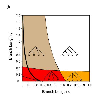
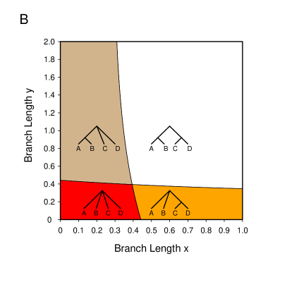
Figure 2: Unresolved zones. The shaded regions are different areas of the unresolved zones leading to different unresolved majority-rule consensus trees. (A) The species tree is (((AB)C)D). A star tree is the limiting consensus tree for the red region, and the orange region corresponds to the tree with the {ABC} clade unresolved. For comparison, the anomaly zone is also plotted as the area under the heavy, dark curve. The anomaly zone cuts across two regions of the unresolved zone, and the area under the line starting from $(x,y)=(0,0.154)$ which creates the approximately triangular region is the part of the anomaly zone with three anomalous gene trees. (B) The species tree is ((AB)(CD)). The unresolved zone in this case is similar in size to that of (a), but there is no anomaly zone for this species tree.

Three taxa.—For the case of three-taxon trees, the MACT is resolved if the probability of the matching tree is greater than 1/2. Using the well-known probability of congruence for a gene tree given a three-taxon species tree, $1-(2/3)e^{-T}$ (Nei, 1987), where $T$ is the length of the one internal branch, this probability is greater than 1/2 if $T>\log(4/3)\approx 0.28768$. If the internal branch length is less than this value, then increasing the number of independent gene trees also increases the probability that the trees do not produce a resolved majority-rule consensus tree, even though the matching gene tree is more likely than any other gene tree.

Four taxa.—For four-taxon trees, the branch lengths needed for a clade to be in the MACT can be obtained by setting the probability of the clade to be greater than 1/2 and solving for branch length $y$ in terms of branch length $x$. These clade probabilities are functions of gene tree probabilities and are listed in Table 1. The model four-taxon trees are shown in Figure 1.

Details for deriving conditions for clades to be in the MACT are given in Appendices 1 and 2. First we consider the species tree with topology (((AB)C)D). Following Figure 1, let $x$ be the length of the branch (in coalescent units) ancestral to A and B, but not C, and let $y$ be the length of the other internal branch. Then {ABC} is a clade in the MACT if and only if

$$x>\log(4/3)\hskip 14.22636pt\text{and}\hskip 14.22636pty>\log\left[\frac{2e^{2x}-1}{3e^{3x}-4e^{2x}}\right],$$ (1)

and {AB} is a clade if and only if

$$y>\log\left[\frac{12e^{3x}+2}{9e^{3x}}\right].$$ (2)

These two conditions partition the space of branch lengths into the four possible MACTs for this species tree (Fig. 2A), where $x=\log(4/3)\approx 0.28768$ is a vertical asymptote. The MACT is:

(((AB)C)D) if (1) and (2) both hold,

((ABC)D) if (1) holds and (2) fails,

((AB)CD) if (1) fails and (2) holds,

(ABCD) if (1) and (2) both fail.

Similarly, if the species tree is ((AB)(CD)), with $y$ denoting the length of the branch ancestral to (AB) and $x$ denoting the length of the other internal branch, then (AB) is a clade in the MACT if and only if

$$y>\log\left[\frac{12e^{x}+2}{9e^{x}}\right],$$ (3)

and (CD) is a clade in the MACT if and only if

$$x>\log(4/3)\hskip 14.22636pt\text{and}\hskip 14.22636pty>\log\left[\frac{2}{9e^{x}-12}\right].$$ (4)

Again, these two conditions partition the branch length space into four regions, one for each of the possible MACTs (Fig. 2B), and $x=\log(4/3)$ is also a vertical asymptote for this graph. The MACT is:

((AB)(CD)) if (3) and (4) both hold,

((AB)CD) if (3) holds and (4) fails,

(AB(CD)) if (3) fails and (4) holds,

(ABCD) if (3) and (4) both fail.

Arbitrarily many taxa.—Because equations (1)–(4) characterize all possible MACTs for four taxa, it follows that four-taxon MACTs are never misleading in the sense that a four-taxon MACT never has a clade that is not a clade in the species tree. Due to lack of resolution, however, the MACT may fail to have clades that are in the species tree. Although we have obtained this result by explicit computation for the four-taxon case, the result holds for larger trees:

Theorem 1. (i) The majority-rule asymptotic consensus tree does not have any clades not on the species tree. (ii) For all species tree topologies with $n\geq 3$ taxa, there exist branch lengths for which the majority-rule asymptotic consensus tree is not fully resolved.

The proof of the first part of Theorem 1 is provided in the section on $R^{*}$ trees below since it is a consequence of the consistency of $R^{*}$ consensus (Theorem 3). The second part of Theorem 1 follows for the three- and four-taxon cases from the calculations above. For larger trees, the second part of Theorem 1 follows from the inconsistency of greedy consensus (Theorem 5) and the fact that greedy consensus trees are refinements of majority-rule trees.

The plots in Figure 2 are analogous to the anomaly zone, the region in branch length space in which the most likely gene tree does not match the species tree (Degnan and Rosenberg, 2006, Fig. 2). Note that the region of parameter space in which MACTs are not fully resolved (and therefore do not fully recover the species tree) is considerably larger than the anomaly zone. For example, when we set $x=y$ for the four-taxon asymmetric tree, the largest value of $x$ that is still in the anomaly zone is approximately 0.1568 (Degnan and Rosenberg, 2006); but for majority-rule consensus, $x=y=0.345$ is approximately the largest value for which $x=y$ and the MACT is fully unresolved, and $x=y=0.507$ is the largest value for which the MACT is partially unresolved, equaling ((AB)CD). For the symmetric four-taxon tree, the values $x=y=0.394$ result in a star consensus tree. This is somewhat surprising since these values result in the partially resolved tree ((AB)CD) for the asymmetric species tree. For the asymmetric four-taxon species tree, the anomaly zone is a subset of the zone in which the MACT is unresolved. For the symmetric species tree, the MACT is unresolved, but there is no anomaly zone. For four taxa, it is always the case that if a species tree has an anomalous gene tree, it does not have a fully resolved MACT.

$R^{*}$ Consensus

Three taxa.—In the case of three taxa, we note that the greedy and $R^{*}$ algorithms are equivalent when there are infinitely many loci. For both algorithms, the most frequently occurring clade also determines a three-taxon statement. In the asymptotic case, there is a uniquely occurring most frequent tree. This tree has probability $1-(2/3)e^{-T}>1/3$ (where $T$ is the one internal branch length), and the other two trees each have probability $(1/3)e^{-T}<1/3$. Thus, for the three-taxon case, as the number of loci approaches infinity, the probability that the matching gene tree is the most frequent approaches 1.

Arbitrarily many taxa.—We show that $R^{*}$ consensus trees are consistent estimators of species tree topologies. This consistency is based on the fact that for any set of three taxa, the rooted triple in the species tree is the highest-probability rooted triple in the gene tree distribution.

Lemma 2. Let $\sigma$ be the species tree where $S$ is the set of taxa on $\sigma$. For any A, B, C $\in S$, if $\sigma$ has the grouping (AB)C, then $P_{\sigma}[\text{(AB)C}]>P_{\sigma}[\text{(AC)B}]$.

Proof. Let $\mathcal{J}$ be the set of branches on $\sigma$ on which A and B can join (i.e., either the lineages A and B or the lineages containing A and B can coalesce in $\mathcal{J}$), but on which A and C cannot join. Note that $\mathcal{J}$ is nonempty and that any branch in $\mathcal{J}$ is an ancestor of A and B, and not an ancestor of C. Let $\mathcal{K}$ be the set of branches on which gene lineages A and C can join. Any branch in $\mathcal{K}$ is an ancestor of A and C. Since (AB)C is a rooted triple, any ancestor of A and C is also an ancestor of B. Thus for any branch $k\in\mathcal{K}$, if none of the lineages A, B, and C have joined, they are free to do so on $k$. The probability that A and B join on a branch in $\mathcal{J}$ is positive. If A and B do not join in $\mathcal{J}$, then the probabilities that A and B, A and C, and B and C are the first two of A, B, and C to join in $\mathcal{K}$ are equal since all pairs of lineages in a population are equally likely to coalesce. Thus $P_{\sigma}[\text{(AB)C}]>P_{\sigma}[\text{(AC)B}]$. $\square$

Theorem 3. For a species tree $\sigma$, the $R^{*}$ asymptotic consensus tree has the same topology as $\sigma$.

Proof. By Lemma 2, any rooted triple in the species tree has higher probability in the gene tree distribution than the other two rooted triples for the same set of three taxa. Thus, the set of rooted triples from which the $R^{*}$ tree is constructed is exactly the set of $\binom{n}{3}$ rooted triples in the species tree, where $n$ is the number of taxa. From Steel (1992), a tree topology is uniquely specified by its set of rooted triples, from which it follows that the only tree topology containing the $\binom{n}{3}$ triples is the topology of the species tree itself. $\square$

Proof of Theorem 1. (i) This result follows from Proposition 3 and Theorem 2.14 of Bryant (2003), according to which every clade in the majority rule consensus tree is in the $R^{*}$ tree. Because the MACT and RACT are the majority-rule and $R^{*}$ consensus trees applied to coalescent gene tree probabilities, every clade in the MACT must appear in the RACT. Because in the limit of infinitely many gene trees, the $R^{*}$ tree is fully resolved, it follows that if the MACT has one or more multifurcations, the $R^{*}$ tree is one of the possible resolutions of the MACT. Because the $R^{*}$ tree has the same topology as the species tree (Theorem 3), the MACT either has the species tree topology or one its resolutions has the same topology as the species tree. $\square$

Theorem 3 describes the RACT, which is a mathematical function of gene tree probabilities, and therefore of species tree branch lengths. When an $R^{*}$ consensus tree is computed from data, however, it has some probability of not matching the species tree. For an estimator of a parameter to be statistically consistent, the probability that it gets arbitrarily close to the parameter must approach 1 as the sample size approaches infinity. Theorem 4 describes the behavior of the $R^{*}$ consensus tree constructed from data when the sample size approaches infinity.

Theorem 4. $R^{*}$ consensus is statistically consistent.

The proof of Theorem 4 uses a generalized version of Bonferroni’s inequality, according to which if there are $k$ events each with probability $p=1-q$, the probability that they all occur is greater than or equal to $1-kq$ (Ross, 1998, p. 63).

Proof. It must be shown that for any $\varepsilon>0$, there exists $k$ such that if there are at least $k$ independent gene trees, the probability is greater than $1-\varepsilon$ that all rooted triples in the species tree are also the most frequently occurring rooted triples for each set of three taxa in the collection of gene trees. Let the species tree be $\sigma$ with taxon set $S$. For $n$ taxa, there are $\binom{n}{3}$ sets of three taxa in $S$. Let A, B, and C be three distinct taxa in $S$. Without loss of generality, assume that (AB)C is the $j$th rooted triple on $\sigma$. From Lemma 2, $P_{\sigma}[\text{(AB)C}]>P_{\sigma}[\text{(AC)B}]=P_{\sigma}[\text{(BC)A}]$, where the equality holds by symmetry. Thus $P_{\sigma}[\text{(AB)C}]=1/3+\delta$ and $P_{\sigma}[\text{(AC)B}]=1/3-\delta/2$ for some $\delta>0$. We use $\widehat{P}$ to denote sample proportions of rooted triples. For any $\varepsilon>0$, because sample proportions converge in probability to their parametric values (by the Weak Law of Large Numbers) as the sample size tends to $\infty$, we can choose the number of loci $k_{j}$ such that with probability greater than $1-\varepsilon/\binom{n}{3}$, $\widehat{P}_{\sigma}[\text{(AB)C}]>1/3$, $\widehat{P}_{\sigma}[\text{(AC)B}]<1/3$, and $\widehat{P}_{\sigma}[\text{(BC)A}]<1/3$. Letting $k=\max_{j|j\in\{1,2,\ldots,{n\choose 3}\}}k_{j}$, for any set of three taxa the probability that its most common rooted triple in the gene tree distribution matches the rooted triple in the species tree is greater than $1-\varepsilon/\binom{n}{3}$. The probability that all of the $\binom{n}{3}$ rooted triples in the $R^{*}$ tree are rooted triples in the species tree is therefore greater than $1-\varepsilon$. $\square$

Greedy Consensus

Three taxa.—For the case of three taxa, greedy consensus applied to gene trees is asymptotically guaranteed to result in the species tree as the number of gene trees increases. If the species tree has topology ((AB)C) and the one internal branch has length $T$, a random gene tree has clade (AB) with probability $1-(2/3)e^{-T}>1/3$, whereas (AC) and (BC) each occur with probability less than 1/3. Thus (AB) is always the most probable cherry for this topology, and the GACT always matches the species tree topology. For finitely many loci, greedy and $R^{*}$ consensus are not equivalent because they handle ties differently, with the $R^{*}$ consensus tree sometimes being unresolved.

Four taxa.—For the four-taxon symmetric species tree and for any choice of branch lengths, the GACT has the same topology as the species tree (Appendix 2). If the species tree is (((AB)C)D), then the GACT can be the symmetric tree ((AB)(CD)).

To find the set of branch lengths for which the GACT fails to match the asymmetric species tree topology, let $x$ and $y$ be the lengths of the deeper and more recent internal branches, respectively, for the tree (((AB)C)D) (see Fig. 1A). For this species tree, the region where the GACT is ((AB)(CD)), the “too-greedy” zone, consists of those values of $x$ and $y$ for which the clade $\{\text{CD}\}$ is more probable than the clade $\{\text{ABC}\}$ (see Appendix 2). The values of $x$ and $y$ for which $P(\{\text{CD}\})>P(\{\text{ABC}\})$ are characterized by

$$y<\log\left[\frac{3e^{2x}-2}{18(e^{3x}-e^{2x})}\right].$$ (5)

The right-hand side of this inequality is strictly less than the boundary of the anomaly zone for the tree (((AB)C)D) (Degnan and Rosenberg, 2006, Equation (4)); thus for this tree, the too-greedy zone is a subset of the anomaly zone (Fig. 5).

More than four taxa.—The result that greedy consensus can be misleading in the four-taxon case generalizes to any species topology with more than four taxa. Intuitively, by making some branches long and some short (so that coalescent events occur with probability arbitrarily close to 0 or 1), trees with five or more taxa can be made to behave similarly to the four-taxon asymmetric case. The strategy of the proof is therefore similar to that of Lemma 5 in Degnan and Rosenberg (2006).

Theorem 5. For three-taxon species topologies, and for four-taxon symmetric species topologies, the GACT matches the species tree; for the asymmetric topology with $n=4$ taxa and for every species topology with $n\geq 5$ taxa, greedy consensus is inconsistent.

Lemma 6. The four-taxon asymmetric topology (((AB)C)D) has a set of branch lengths which makes greedy consensus fail to match the species tree.

Proof. This set is explicitly derived in Appendix 2 and is given in equation (5) and Figure 5. $\square$

Lemma 7. For every bifurcating species tree with $n\geq 5$ taxa and every $k\geq 1$ with $2^{k+1}<n$, there is a node with $c$ terminal descendants, where $2^{k}<c<2^{k+1}+1$.

Proof. For all $k$ satisfying $2^{k+1}+1\leq n$, the root has $n\geq 2^{k+1}+1$ terminal descendants. Let $\mathcal{N}_{0}$ denote the root node, and let $\mathcal{N}_{1}$ denote the internal node immediately descended from the root with the larger number of terminal descendants (choosing arbitrarily in case of a tie). Similarly let $\mathcal{N}_{2}$ be the internal node (if it exists) immediately descended from $\mathcal{N}_{1}$ with the larger number of terminal descendants. Continue this process until a node $\mathcal{N}_{m}$ ($m\geq 0$) is reached which has at least $2^{k+1}+1$ terminal descendants, but neither of whose immediate descendant nodes has more than $2^{k+1}$ terminal descendants. Call $\mathcal{N}_{m}$ the “minimal node”. It follows that at least one of the immediate descendant nodes of the minimal node has more than $2^{k}$ terminal descendants (since otherwise the minimal node would have at most $2(2^{k})<2^{k+1}+1$ descendants). Thus at least one immediate descendant of the minimal node has $c$ terminal descendants with $2^{k}<c<2^{k+1}+1$. $\square$

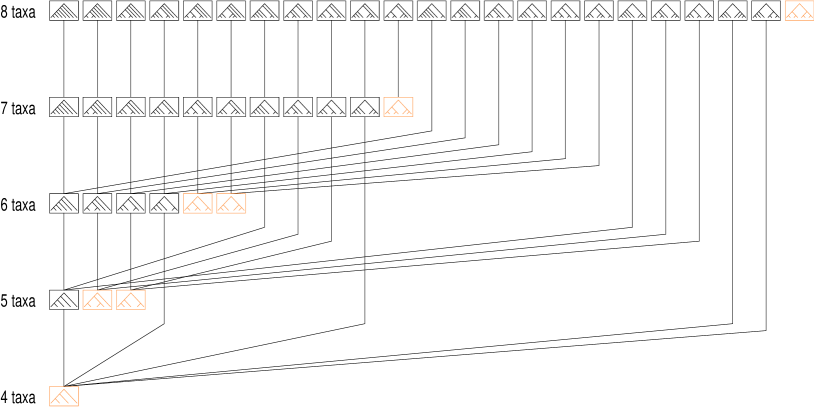
Figure 3: Reduction of topologies used in the proof of Lemma 9. If two trees are connected by an edge, then the topology with the smaller number of leaves is a left subtree of the larger tree.

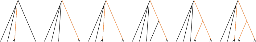
Figure 4: Reduction of the remaining trees from Figure 3 to the four-taxon asymmetric case. Branches in orange are made long enough that all lineages on these branches coalesce with probability arbitrarily close to 1.

Lemma 8. If for some $k\geq 2$, all species tree topologies with $n$ taxa, $n\in\{2^{k}+1,\dots,2^{k+1}\}$, have a nonempty too-greedy zone, then all species tree topologies with $n>2{k+1}$ (and thus $n\geq 2^{k}+1$) taxa have a nonempty too-greedy zone.

Proof. Assume there exists $k\geq 2$ such that all species tree topologies with $n\in\{2^{k}+1,\dots,2^{k+1}\}$ taxa have a nonempty too-greedy zone, i.e., that there exist branch lengths for which the GACT does not match the species tree topology. By Lemma 7, any species tree $\sigma$ with more than $2^{k+1}$ ($k\geq 1$) taxa $S$ has some node $\mathcal{N}$ with $c$ terminal descendants, where $c\in\{2^{k}+1,\dots,2^{k+1}\}$. Let $\sigma_{\mathcal{N}}$ denote the species tree rooted at $\mathcal{N}$ and let $S_{\mathcal{N}}$ denote the taxa labeling the tips of $\sigma_{\mathcal{N}}$. By assumption, $\sigma_{\mathcal{N}}$ has a nonempty too-greedy zone.

Make the lengths of all branches outside of $\sigma_{\mathcal{N}}$ long enough that the probability that all lineages on these long branches coalesce is greater than $1-\varepsilon$, where $\varepsilon$ is chosen so that $1-\varepsilon>1/2$ and $1-\varepsilon$ is greater than the probability of any clade within $\sigma_{\mathcal{N}}$ (i.e., any clade which is a proper subset of $S_{\mathcal{N}}$). Because the greedy consensus tree is a refinement of the majority-rule consensus tree, all clades which include taxa outside of $S_{\mathcal{N}}$, and the clade consisting of all taxa in $S_{\mathcal{N}}$, are included in the GACT. When ranking clade probabilities as is required for the algorithm for constructing the GACT, these clades are added before the clades consisting of taxa which are proper subsets of $S_{\mathcal{N}}$. Thus eventually the list of candidate clades consists only of proper subsets of $S_{\mathcal{N}}$. When clades are accepted from this list, by assumption we accept at least one clade to be in the GACT which is not on $\sigma$. Thus there exist branch lengths on $\sigma$ for which the GACT does not match the species tree. $\square$

Lemma 9. For any species tree topology with 5, 6, 7, or 8 taxa, there exists a set of branch lengths for which the greedy asymptotic consensus tree does not match the species tree.

Proof. This is shown by reduction to the four-taxon asymmetric case. For each species tree topology with 5, 6, 7, or 8 taxa, some branches can be made long, and some short so as to produce the same inconsistencies as in the four-taxon case. Most cases are shown in Figure 3. Here a topology with $n$ taxa is connected by an edge to a topology with fewer than $n$ taxa if the smaller topology is the left subtree—from the node which is the immediate left-descendant of the root—of the larger topology. In this case, for any $\epsilon>0$, any branches on the larger topology not in the left subtree can be made arbitrarily long. Thus any lineages available to coalesce on long branches do coalesce with probability greater than $1-\varepsilon$. Remaining clades then have the same order of probabilities as on the left subtree, and thus are accepted by the greedy algorithm in the same order as on the left subtree.

If the greedy consensus algorithm returns a nonmatching tree for the smaller tree, it also does so for the larger tree since the ranking of the remaining clades by frequencies is eventually the same (once the high probability clades have already been added on the larger tree). This process of reducing trees can be repeated until one of the trees colored orange (which have no edges connecting to a smaller tree) is reached.

It then remains to be shown that GACT does not match the species tree for the remaining orange trees from Figure 3. This is already shown explicitly for the four-taxon case (Lemma 6). For the other trees, these can again be reduced to the four-taxon case by choosing certain edges to be long and others short. This is shown in Figure 4. By choosing the long, orange branches to have large branch lengths, the probability that all available lineages coalesce on a branch can be made greater than $1-\varepsilon/(2m)$, where $m$ is the number of long branches on a tree. This makes the probability that all available lineages on long branches coalesce greater than $1-\varepsilon/2$. Since only counterexamples are needed to show that the greedy consensus algorithm can return a nonmatching tree, it is sufficient to note that branches can be chosen to be short enough using eq. 5 or Figure 5 for the four-taxon asymmetric tree to make the greedy consensus algorithm fail to return the tree matching the species tree with probability greater than $1-\varepsilon/2$. Making the black internal branches sufficiently short, the probability is greater than $1-\varepsilon$ that the the entire tree returned by the greedy consensus algorithm returns fails to match the species tree topology. $\square$

Proof of Theorem 5. The result for three taxa follows from the fact that the matching gene tree has the highest probability of the three possible gene trees. The four-taxon asymmetric case is covered in Lemma 6. The four-taxon symmetric case is shown to be consistent in Appendix 2 by showing that for all branch lengths, (AB) and (CD) are the two most probable clades. We have shown that all cases with $n=5,6,7,\text{or }8$ taxa have too-greedy zones (Lemma 9). From Lemma 8, this verifies by induction that all cases with $n\geq 5$ taxa have such zones. $\square$

Proof of Theorem 1(ii). The GACT and MACT are each examples of greedy and majority-rule consensus trees, respectively. It follows that if the MACT is fully resolved, then it is the same as the GACT since greedy consensus trees are refinements of majority-rule consensus trees (Bryant, 2003). However, by Theorem 5, for any species tree topology with $n\geq 5$ taxa, there exist branch lengths for which the GACT has a clade not on the species tree, and therefore cannot be equivalent to the MACT (by Theorem 1(i)). Therefore a sufficient condition for the MACT to be unresolved is for the GACT to not match the species tree. Since exact conditions for the MACT to not be fully resolved were obtained earlier for smaller trees (the internal branch length being no greater than $\log(4/3)$ for three-taxon trees and one of eqs. (1)–(4) to fail for four-taxon trees), the result follows for any species tree with $n\geq 3$ taxa. $\square$

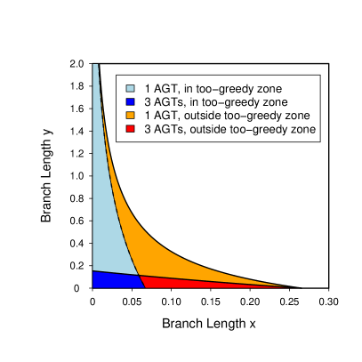
Figure 5: The too-greedy zone. The upper curve is the boundary of the anomaly zone for the species tree (((AB)C)D). For points below this curve, there is either one or three anomalous gene trees (AGTs). The two blue regions to the left of the curve which extends from roughly $(x,y)=(0.067,0.0)$ to $(0.0078,2.0)$ constitute the too-greedy zone, where the GACT is ((AB)(CD)).

Finite Numbers of Loci

Theory

The asymptotic consensus trees occur in the limit as the number of loci approaches infinity. What happens with a finite number of loci? In this case, we can examine the behavior of consensus trees from a theoretical point of view by considering all possible finite samples of gene trees. The probability of a particular consensus tree is the sum of the probabilities of those samples of gene trees that result in that consensus tree. These probabilities can be determined by noting that a sample of independent loci has a multinomial distribution, where the categories are the gene tree topologies, and the probabilities are given by the theory of the multispecies coalescent (Degnan and Salter, 2005).

To compute the probability of a consensus tree given a finite sample of $\ell$ gene trees, let $\ell_{i}$,$i=1,\dots,k$ be the number of times gene tree $i$ is observed, where $\sum_{i}\ell_{i}=L$, and there are $k$ possible gene tree topologies. let $c(\ell_{1},\dots,\ell_{k})$ denote the consensus tree resulting from a particular sample. The probability that a sample results in the consensus tree having topology $\mathcal{T}$ is therefore

$$\sum_{\begin{subarray}{c}\ell_{1},\ldots,\ell_{k}\geq 0\\ \ell_{1}+\dots+\ell_{k}=l\end{subarray}}\frac{\ell!}{\ell_{1}!\cdots\ell_{k}!}p_{1}^{\ell_{1}}\cdots p_{k}^{\ell_{k}}\;I(c(\ell_{1},\dots,\ell_{k})=\mathcal{T})$$ (6)

where $I$ is an indicator that the consensus tree has topology $T$, $p_{i}$ is the gene tree probability for the $i$th topology, and the sum is over all nonnegative integer solutions to $\ell_{1}+\cdots+\ell_{k}=\ell$. There are $\binom{\ell+k-1}{k-1}$ terms in the sum (Ross, 1998, p. 13). For four taxa and 25 loci, the sum has approximately $1.51\times 10^{10}$ terms.

To compute the probabilities of finite-sample greedy consensus trees, probabilities of resolutions of ties must also be taken into account. This can be done by summing over all possible tie-breaks and treating each possible tie-break as equally likely, rather than randomly breaking ties. The probability of the greedy consensus tree having topology $\mathcal{T}$ can therefore be written as

$$\begin{split}\sum_{\begin{subarray}{c}\ell_{1},\ldots,\ell_{k}\geq 0\\ \ell_{1}+\dots+\ell_{k}=l\end{subarray}}\frac{\ell!}{\ell_{1}!\cdots\ell_{k}!}p_{1}^{\ell_{1}}\cdots p_{k}^{\ell_{k}}\Biggl{[}\sum_{b_{1}\in B_{1}}\dots\sum_{b_{r}\in B_{r}(b_{1},\dots,b_{r-1})}\\ \prod_{j=1}^{r}\Pr(b_{j})I(c(\ell_{1},\dots,\ell_{k},b_{1},\dots,b_{r})=\mathcal{T})\Biggr{]},\end{split}$$

where $B_{j}$ denotes the set of possible tie-breaks in the $j$th round, $b_{j}$ denotes one way (out of $|B_{j}|$ possible ways, where $|B_{i}|$ is the number of elements in $B_{j}$) of breaking up a set of tied clade frequencies in the $jth$ round (out of $r$ rounds) of choosing clades for the greedy consensus tree, and $\Pr(b_{j})=1/|B_{j}|$ is the probability of a particular tie break. In general, the set $B_{j}$ is a function of the choices $b_{1},\dots,b_{j-1}$ in preceding rounds of tie-breaks, since the possible tie breaks in a given round may depend on how previous ties were resolved. For $n$-taxon trees, there are $n-2$ rounds of tie breaks, assuming the case when no tie breaks are necessary (i.e., there is one clade on the list which is most frequent) is treated as a trivial tie break with $|B_{j}|=1$. For example, for four-taxon trees, there are two rounds of tie breaks. The function $c$ in eq. 7 has been given additional arguments (compared with eq. 6) so that the consensus tree is a function of both the gene tree frequencies and the tie-breaks.

Because there are a finite number of trees and consensus trees are computed for every sample, many samples include gene trees which imply incompatible sets of rooted triples due to there being ties in the most frequently occurring rooted triple for a given set of taxa. In these cases, the $R^{*}$ algorithm returns a tree which is partially or completely unresolved. For example, if there are four input gene trees: (((AB)C)D), (((AD)C)B), (((BC)A)D), and (((CD)A)B), then the rooted triples (AD)B and (AB)D each occur twice; thus the $R^{*}$ consensus tree is unresolved with respect to the relationships between A, B, and D. Similarly the rooted triples (BC)D and (CD)B each occur twice. However, the rooted triple (AC)B occurs twice whereas (AB)C and (BC)A each occur once, so the $R^{*}$ consensus tree has the rooted triple (AC)B. Similarly, (AC)D occurs in the $R^{*}$ tree. Thus the $R^{*}$ consensus tree for this set of gene trees is the partially unresolved tree ((AC)BD). The majority-rule tree for this set of input trees is completely unresolved, and the greedy consensus tree returns each of the four input trees with probability 0.25.

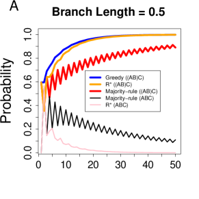
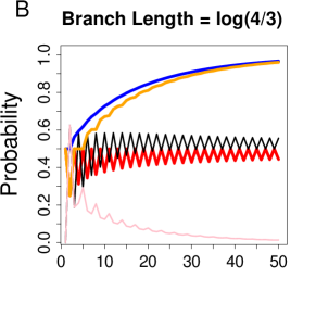
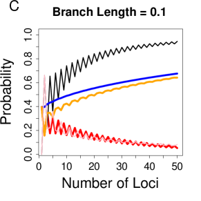
Figure 6: Species tree ((AB)C)—Probabilities of consensus trees from finite numbers of known gene trees. Each plot shows the probability that each of the three consensus methods will return either the species topology, ((AB)C) or a star tree ($R^{*}$ and majority-rule only). The legend in (A) applies to each of the three plots.

Examples

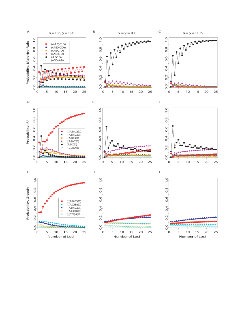
Figure 7: Species tree (((AB)C)D)—Probabilities of consensus trees as functions of sample size (number of loci). One consensus algorithm is used for each row of plots, and one set of branch lengths is used for each column. For the majority-rule and $R^{*}$ algorithms, there are 26 possible four-taxon consensus trees, including 15 fully resolved trees and 11 trees not fully resolved. The graphs only show some of the more frequently occurring consensus trees; consequently probabilities do not add to 1.0. The legends in the lefthand column apply to the three plots in their corresponding rows.

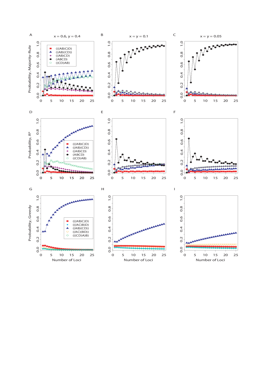
Figure 8: Species tree ((AB)(CD))—Probabilities of consensus trees as functions of sample size (number of loci). One consensus algorithm is used for each row of plots, and one set of branch lengths is used for each column. For the majority-rule and $R^{*}$ algorithms, there are 26 possible four-taxon consensus trees, including 15 fully resolved trees and 11 trees not fully resolved. The graphs only show some of the more frequently occurring consensus trees; consequently probabilities do not add to 1.0. The legends in the lefthand column apply to the three plots in their corresponding rows.

Three taxa.—We illustrate the case of finite loci using three (Fig. 6) and four taxa (Figs. 7 and 8). With three taxa, there is only one internal branch length, and this determines all gene tree probabilities, with the probability that the gene tree matches the species tree being $1-(2/3)e^{-T}$, where $T$ is the length of the internal branch. We used ((AB)C) as the species tree with branch lengths of $0.5,\log(4/3)\approx 0.288,\text{ and }0.1$, corresponding to matching probabilities of 0.596, 0.5, and 0.397, respectively.

For the branch length of 0.5, the majority of loci (almost 60%) are likely to have the matching topology; thus, given enough loci, all three methods (majority-rule, $R^{*}$, and greedy) are expected to have a high probability of returning the matching tree. This does in fact occur, with the greedy consensus tree having the highest probability for any given number of loci. The $R^{*}$ method has the second-best performance, although by 50 loci, the greedy and $R^{*}$ algorithms have roughly equivalent performance. When the branch length was chosen such that the probability of matching was 0.5 (Fig. 6B, with the two nonmatching trees each having probability 0.25), majority-rule was stuck between returning the correct tree and the star tree. This was not surprising since ((AB)C) by design does not occur more than 50% of the time. The pattern for this case, as well as for the branch length of 0.1 (Fig. 6C), continues for greedy and $R^{*}$ consensus, with greedy having the best performance, and $R^{*}$ slowly approaching greedy as the number of loci increases (and therefore the probability of ties decreases). Also, for the branch length of 0.1, no tree has greater than 50% probability of occurring, and therefore majority-rule becomes increasingly likely to return a star tree as the number of loci increases.

Four taxa.—Figure 7 shows the behavior of the three consensus methods as the number of loci increases when the species tree is (((AB)C)D), and Figure 8 shows the same consensus methods when the species tree is ((AB)(CD)). The results of the two figures are similar, although the methods generally perform better with the symmetric species tree.

Figure 7A suggests that large numbers of loci might be needed before one majority-rule consensus tree becomes the most probable. Figures 7B,C and 8B,C, show that majority-rule consensus can fairly quickly converge to a star phylogeny even though the probability of a star phylogeny decreases under $R^{*}$ and greedy consensus.

For majority-rule trees, there is also an effect of having an odd or even sample size, where even sample sizes tend to give higher probabilities to unresolved trees. This occurs because even sample sizes increase the opportunity for ties in the number of times two (or more) clades are observed, and in these cases neither clade can be in the majority. This has the somewhat surprising result that a consensus tree can be less likely to match the species tree in a sample of $2n$ loci than in a sample of $2n-1$ loci (although in being more likely to have an unresolved tree, it is also less likely to produce a tree resolved in a way that conflicts with the species tree). For the symmetric species topology with branch lengths of $x=0.6$ and $y=0.4$, note that the majority-rule consensus tree is more likely to be the species tree topology ((AB)(CD)) than any other topology if the sample size is odd, but for even sample sizes up to 25 loci, the unresolved tree ((AB)CD) is roughly tied in probability with ((AB)(CD)). This is consistent with Figure 2B, in which the point $(x,y)=(0.6,0.4)$ is close the boundary between the regions for ((AB)(CD)) and (AB(CD)). However, if the number of loci is sufficiently large, majority-rule consensus is expected to return the resolved tree ((AB)(CD)) that matches the species topology, since the point $(x,y)=(0.6,0.4)$ is slightly outside the zone where the MACT is unresolved. This can be verified from equations 3 and 4.

As the number of loci increases, the finite-sample $R^{*}$ trees (Figs. 7D–F and Figs. 8D–F) show increasing probability of matching the species tree topology, regardless of how short the branches are, including for branch lengths that are in the anomaly zone, $(x,y)=(0.1,0.1)$, and the too-greedy zone, $(x,y)=(0.05,0.05)$. This agrees with our theoretical expectations of $R^{*}$ consensus trees (Theorem 4); however, the increase in probability is very slow. For example, when $(x,y)=(0.1,0.1)$ and the species tree is asymmetric (Fig. 7E), the two trees most likely to be returned are (ABCD) and ((AB)CD) until there are 23 loci, at which point the matching topology (((AB)C)D) changes from being the third to the second most probable topology. The star tree (ABCD) has the highest probability for 11 and fewer loci, and as a trend is decreasing in probability as the sample size increases. The tree ((AB)CD), however, is still increasing in probability at 25 loci; thus large numbers of loci might be needed for $R^{*}$ to show a clear preference for the matching tree. The probability that $R^{*}$ returns the species tree topology grows more slowly when $(x,y)=(0.05,0.05)$ (Figs. 7F, 8F); however, it is the only one of the three methods for which the probability is increasing with those branch lengths.

Greedy consensus trees show more smoothly increasing probabilities of returning the matching tree for branch lengths outside of the too-greedy zone (Figs. 7G,H and Figs. 8G–I). When the species tree is (((AB)C)D) and $(x,y)=(0.1,0.1)$ (Fig. 7H), the gene tree ((AB)(CD)) is more probable than the matching tree, and here greedy consensus is slightly more likely to return this tree for small samples; but the matching tree becomes the most probable greedy consensus tree with 11 or more loci. However, for this species tree, the more extreme branch lengths of $(x,y)=(0.05,0.05)$ make increasing the number of loci more likely to result in greedy consensus returning the nonmatching tree ((AB)(CD)) (Fig. 7I). These results are consistent with our expectations based on the too-greedy zone (Fig. 5).

Discussion

Using coalescent probabilities to determine asymptotic consensus trees enables the prediction of what occurs when consensus trees are constructed from gene trees from many independent loci. We have obtained results for the three types of asymptotic consensus trees considered: majority-rule, $R^{*}$, and greedy (Theorems 1, 3, and 5, respectively), which describe the fact that with an infinite number of loci, MACTs might be unresolved, GACTs might be nonmatching, and RACTs always match the species tree. These results have implications for a common goal of phylogenetics: the inference of species trees.

Estimating Species Trees

Although concatenation of sequences is perhaps the most widely used method of estimating species trees, there are several current alternatives to concatenation for inferring species trees. These include minimizing deep coalescence (Maddison and Knowles, 2006), finding the joint posterior of the species tree and gene trees from the coalescent model in a Bayesian framework (Liu and Pearl, 2007), using the most ancient speciation times compatible with the set of inferred coalescent times on a set of gene trees (called the “maximum tree” by Liu and Pearl (2007) or “GLASS tree” by Mossel and Roch (2007)), and using probabilities of gene tree topologies to approximate the species likelihood (Carstens and Knowles, 2007; Carling and Brumfield, 2008). These methods are designed estimate species trees when there is gene tree conflict due to incomplete lineage sorting, and they do not assume that sequence data are generated under a single gene tree topology.

Theorem 4 suggests a statistically consistent method for building species tree topologies from gene tree topologies (assuming known gene trees). This involves inferring all rooted triples and then applying a method such as that of Bryant and Berry (2001) to build up the tree by the $\binom{n}{3}$ rooted triples.

Although this method does not estimate branch lengths on the species tree, rooted triples could also be used to estimate internal branch lengths on the species tree by using $P_{\sigma}[\text{(AB)C}]=1-(2/3)e^{-T}$, where $T$ is the length separating the MRCA of A, B, and C from the MRCA of A and B. Thus, the frequency of each rooted triple in the observed set of gene trees could be used to estimate species divergence times, from which the species tree (including topology) could be constructed; or, given a species tree topology, the set of branch lengths most compatible with the observed rooted triples could be determined using a criterion such as maximum likelihood or least squares.

Using majority-rule trees to estimate species trees from finitely many loci is expected to not be misleading, but is likely to result in a tree that is at least partially unresolved. It is thus expected to be a conservative estimate of the species tree, with little power to resolve some clades for some sets of branch lengths.

a

Mutation and recombination

In this paper, we have not considered the roles of mutation and recombination and the resulting uncertainty that occurs when gene trees are inferred from sequence data. When gene trees are estimated and the underlying species tree has short branches, some gene trees are expected to not be fully resolved due to insufficient sequence divergence. Due to the inherent stochasticity in sequence evolution, there will also be some incorrectly inferred gene trees. For finite numbers of genes, these factors would tend to increase the probability that majority-rule consensus trees would have some lack of resolution, whether or not the true MACT was fully resolved. If the MACT is a star tree, we speculate that mutation would cause convergence to a star tree occur more quickly as the number of loci is increased. If the MACT does have some resolved clades, then uncertainty in the gene trees would be expected to increase the number of loci needed to have a high probability that the majority-rule tree is correctly resolved. We expect similar effects for $R^{*}$ and greedy consensus trees, but ultimately, the effects of mutation on constructing consensus trees could be assessed by simulating sequence data for independent gene trees evolving in the same species tree.

When recombination occurs within genes, different topologies may exist for different segments within a gene, further complicating the distribution of site patterns (Wiuf et al., 2001).

Conclusions

Our results show that when there is sufficient gene tree discordance due to incomplete lineage sorting, majority-rule consensus trees can have a high probability of being at least partially unresolved, and the probability of being unresolved can approach 1 as the number of genes increases indefinitely. However, the MACT is never resolved incorrectly; that is, it never has a clade not supported on the species tree. We therefore describe the MACT as not misleading; however, it is not consistent, because statistical consistency implies that an estimator gets arbitrarily close to a parameter (e.g., a fully resolved species tree) with probability approaching 1 as the sample size increases.

The fact that under the multispecies coalescent, $R^{*}$ trees are asymptotically guaranteed to be fully resolved and to match the species tree topology means that the $R^{*}$ procedure is not only not misleading, but is also a statistically consistent estimator of the species tree topology. This is remarkable considering that $R^{*}$ trees (which are defined for any collection of trees) are based only minimally on a model of species tree-gene tree relationships. The only feature of the multispecies coalescent model used in proving the consistency of the $R^{*}$ method is the fact that in this model, three-taxon relationships that occur in the species tree are also expected to occur in the gene tree distributions. Thus, although $R^{*}$ consensus trees are consistent without explicitly incorporating gene tree probabilities into its algorithm for constructing trees, the $R^{*}$ consensus tree is not necessarily robust to violations of assumptions in the coalescent, such as the absence of population structure along ancient internal edges.

Finally, greedy consensus trees can be increasingly likely (as the number of gene trees increases) to have a topology that differs from that of the species tree. Thus greedy consensus trees can be positively misleading if used as estimators of species trees. However, for four taxa, the region of parameter space in which greedy consensus fails to return the true tree—the too-greedy zone—is smaller than the anomaly zone; hence greedy consensus offers some robustness to gene tree discordance that may cause other methods to fail to recover the species tree. In addition, the greedy consensus method outperformed our other methods for branch lengths outside of the too-greedy zone. To test these consensus methods in practice will require examining their performance in the presence of mutation (both from real and simulated sequence data) that can cause gene trees to be estimated with uncertainty rather than treated as known. Although in our results, $R^{*}$ consensus outperformed majority-rule consensus, for $R^{*}$ and greedy consensus there may be a tradeoff between consistency and speed of convergence, with greedy consensus being the quicker to converge yet statistically consistent, and with $R^{*}$ consensus being slow to converge yet statistically consistent.

Table 1: Probabilities of four-taxon gene tree topologies, clades, and rooted triples for the species tree (((AB)C)D) with different branch lengths. A clade (rooted triple) probability is the sum of probabilities of gene tree topologies which have the clade (rooted triple). Branch lengths are as in the model species tree in Figure 1A. An asterisk indicates that a clade has probability greater than 1/2, and would therefore be represented in the MACT.

				Branch lengths $(x,y)$
Gene tree	Probability			$(.6,.4)$	$(.4,.6)$	$(.8,.3)$	$(.3,.3)$	$(.1,.1)$	$(.05,.05)$
(((AB)C)D)		$p_{1}$		.316	.319	.321	.212	.104	.079
(((AB)D)C)		$p_{2}$		.109	.144	.087	.122	.091	.075
(((AC)B)D)		$p_{3}$		.107	.069	.140	.081	.066	.061
(((AC)D)B)		$p_{4}$		.049	.043	.048	.058	.062	.060
(((AD)B)C)		$p_{5}$		.006	.009	.004	.017	.037	.045
(((AD)C)B)		$p_{6}$		.006	.009	.004	.017	.037	.045
(((BC)A)D)		$p_{7}$		.107	.069	.140	.081	.066	.061
(((BC)D)A)		$p_{8}$		.049	.043	.048	.058	.062	.060
(((BD)A)C)		$p_{9}$		.006	.009	.004	.017	.037	.045
(((BD)C)A)		$p_{10}$		.006	.009	.004	.017	.037	.045
(((CD)A)B)		$p_{11}$		.006	.009	.004	.017	.037	.045
(((CD)B)A)		$p_{12}$		.006	.009	.004	.017	.037	.045
((AB)(CD))		$p_{13}$		.115	.153	.094	.139	.128	.121
((AC)(BD))		$p_{14}$		.055	.052	.052	.075	.099	.105
((AD)(BC))		$p_{15}$		.055	.052	.052	.075	.099	.105
Clade
{AB}		$p_{1}+p_{2}+p_{13}$		*.541*	*.616*	.499	.473	.322	.275
{AC}		$p_{3}+p_{4}+p_{14}$		.211	.165	.239	.213	.227	.226
{AD}		$p_{5}+p_{6}+p_{15}$		.067	.071	.059	.108	.174	.196
{BC}		$p_{7}+p_{8}+p_{15}$		.110	.104	.103	.149	.227	.226
{BD}		$p_{9}+p_{10}+p_{14}$		.067	.071	.059	.108	.174	.196
{CD}		$p_{11}+p_{12}+p_{13}$		.128	.171	.098	.172	.202	.212
{ABC}		$p_{1}+p_{3}+p_{7}$		*.530*	.458	*.601*	.373	.236	.201
{ABD}		$p_{2}+p_{5}+p_{9}$		.121	.162	.094	.155	.165	.166
{ACD}		$p_{4}+p_{6}+p_{11}$		.061	.061	.055	.091	.136	.151
{BCD}		$p_{8}+p_{10}+p_{12}$		.061	.061	.055	.091	.136	.151
Rooted triple
(AB)C		$p_{1}+p_{2}+p_{5}+p_{9}+p_{13}$		.553	.634	.506	.506	.397	.366
(AC)B		$p_{3}+p_{4}+p_{6}+p_{11}+p_{14}$		.223	.183	.247	.247	.302	.317
(BC)A		$p_{7}+p_{8}+p_{10}+p_{12}+p_{15}$		.223	.183	.247	.247	.302	.317
(AB)D		$p_{1}+p_{2}+p_{3}+p_{7}+p_{13}$		.755	.755	.778	.634	.454	.397
(AD)B		$p_{4}+p_{5}+p_{6}+p_{11}+p_{15}$		.123	.123	.111	.183	.273	.302
(BD)A		$p_{8}+p_{9}+p_{10}+p_{12}+p_{14}$		.123	.123	.111	.183	.273	.302
(AC)D		$p_{1}+p_{3}+p_{4}+p_{7}+p_{14}$		.634	.553	.700	.506	.397	.366
(AD)C		$p_{2}+p_{5}+p_{6}+p_{9}+p_{15}$		.183	.223	.150	.247	.302	.317
(CD)A		$p_{8}+p_{10}+p_{11}+p_{12}+p_{13}$		.183	.150	.247	.223	.302	.317
(BC)D		$p_{1}+p_{3}+p_{7}+p_{8}+p_{15}$		.634	.553	.700	.506	.397	.366
(BD)C		$p_{2}+p_{5}+p_{9}+p_{10}+p_{14}$		.183	.223	.150	.247	.302	.317
(CD)B		$p_{4}+p_{6}+p_{11}+p_{12}+p_{13}$		.183	.223	.150	.247	.302	.317

Table 2: Probabilities of four-taxon gene trees, clades, and rooted triples as functions of terms $g_{ij}(T)$. The branch lengths $x$ and $y$ are as in Figure 1A. The probabilities of clades (rooted triples) are obtained by adding the probabilities of gene trees for which have the clade (rooted triple, see Table 1). For each entry in the table, the left and right numbers are the coefficients of the $g_{ij}(T)$ terms for the species trees (((AB)C)D) and ((AB)(CD)), respectively.

Gene Tree	$g_{21}(y)g_{21}(x)$	$\frac{1}{3}g_{21}(y)g_{22}(x)$	$\frac{1}{3}g_{22}(y)g_{21}(x)$	$\frac{1}{18}g_{22}(y)g_{22}(x)$	$\frac{1}{3}g_{22}(y)g_{31}(x)$	$\frac{1}{9}g_{22}(y)g_{32}(x)$	$\frac{1}{18}g_{22}(y)g_{33}(x)$
1. (((AB)C)D)	1,0	1,1	0,0	0,1	1,0	1,0	1,0
2. (((AB)D)C)	0,0	1,1	0,0	0,1	0,0	1,0	1,0
3. (((AC)B)D)	0,0	0,0	0,0	0,1	1,0	1,0	1,0
4. (((AC)D)B)	0,0	0,0	0,0	0,1	0,0	1,0	1,0
5. (((AD)B)C)	0,0	0,0	0,0	0,1	0,0	0,0	1,0
6. (((AD)C)B)	0,0	0,0	0,0	0,1	0,0	0,0	1,0
7. (((BC)A)D)	0,0	0,0	0,0	0,1	1,0	1,0	1,0
8. (((BC)D)A)	0,0	0,0	0,0	0,1	0,0	1,0	1,0
9. (((BD)A)C)	0,0	0,0	0,0	0,1	0,0	0,0	1,0
10. (((BD)C)A)	0,0	0,0	0,0	0,1	0,0	0,0	1,0
11. (((CD)A)B)	0,0	0,0	0,1	0,1	0,0	0,0	1,0
12. (((CD)B)A)	0,0	0,0	0,1	0,1	0,0	0,0	1,0
13. ((AB)(CD))	0,1	1,1	0,1	0,2	0,0	1,0	2,0
14. ((AC)(BD))	0,0	0,0	0,0	0,2	0,0	1,0	2,0
15. ((AD)(BC))	0,0	0,0	0,0	0,2	0,0	1,0	2,0
Clade
{AB}	1,1	3,3	0,1	0,4	1,0	3,0	4,0
{AC}	0,0	0,0	0,0	0,4	1,0	3,0	4,0
{AD}	0,0	0,0	0,0	0,4	0,0	1,0	4,0
{BC}	0,0	0,0	0,0	0,4	1,0	3,0	4,0
{BD}	0,0	0,0	0,0	0,4	0,0	1,0	4,0
{CD}	0,1	1,1	0,3	0,4	0,0	1,0	4,0
{ABC}	1,0	1,1	0,0	0,3	3,0	3,0	3,0
{ABD}	0,0	1,1	0,0	0,3	0,0	1,0	3,0
{ACD}	0,0	0,0	0,1	0,3	0,0	1,0	3,0
{BCD}	0,0	0,0	0,1	0,3	0,0	1,0	3,0
Rooted Triple
(AB)C	1,1	3,3	0,1	0,6	1,0	3,0	6,0
(AC)B	0,0	0,0	0,1	0,6	1,0	3,0	6,0
(BC)A	0,0	0,0	0,1	0,6	1,0	3,0	6,0
(AB)D	1,1	3,3	0,1	0,6	3,0	5,0	6,0
(AD)B	0,0	0,0	0,1	0,6	0,0	2,0	6,0
(BD)A	0,0	0,0	0,1	0,6	0,0	2,0	6,0
(AC)D	1,0	1,1	0,0	0,6	3,0	5,0	6,0
(AD)C	0,0	1,1	0,0	0,6	0,0	2,0	6,0
(CD)A	0,1	1,1	0,3	0,6	0,0	2,0	6,0
(BC)D	1,0	1,1	0,0	0,6	3,0	5,0	6,0
(BD)C	0,0	1,1	0,0	0,6	0,0	2,0	6,0
(CD)B	0,1	1,1	0,3	0,6	0,0	2,0	6,0

Appendix 1: Majority-Rule Unresolved Zones, Species Tree (((AB)C)D)

In this appendix we derive conditions for which the MACT is unresolved for the four-taxon species trees (((AB)C)D) and ((AB)(CD)). This is done by finding branch lengths for which there exist clades with probability greater than 1/2. First, the following result about cherries is useful, which is analogous to Proposition 1 and has a similar proof.

Proposition 10. Let $\sigma$ be the species tree where $S$ is the set of taxa on $\sigma$. Then for any A, B, C $\in S$, if {AB} is a cherry on $\sigma$, then $P_{\sigma}[\text{\{AB\}}]>P_{\sigma}[\text{\{AC\}}]$.

Proof. The proof is very similar to the proof of Lemma 2.

Remark 11. If {AB} is a cherry on the species tree $\sigma$, then for any taxon C, $P_{\sigma}[\text{\{AC\}}]=P_{\sigma}[\text{\{BC\}}]<1/3$.

The equality holds by symmetry; the inequality follows from Proposition 10.

To find branch lengths for the species tree (((AB)C)D) where the MACT is resolved, consider the probabilities of clades {ABC} and {AB}. Table 1 lists the probability that A, B, and C are monophyletic as $p_{1}+p_{3}+p_{7}$, where $p_{i}$ is the probability of gene tree $i$ in the same table, because for gene trees 1, 3, and 7 (and only these gene trees), these three taxa are monophyletic. Table 2 can be used to compute probabilities of gene trees, clades, or rooted triples for four-taxon trees as linear combinations of products of the terms $g_{i,j}(T)$, which denote the probability that $i$ lineages coalesce into $j$ lineages within $T$ coalescent units, where $i\geq j\geq 1$, and $T>0$. For $i=2,3$, the $g_{ij}(t)$ functions are (Tavaré, 1984; Pamilo and Nei, 1988):

$$g_{21}(T) =1-e^{-T}\hskip 7.22743pt g_{31}(T)=1-\frac{3}{2}e^{-T}+\frac{1}{2}e^{-3T}$$

$$g_{22}(T) =e^{-T} g_{32}(T)=\frac{3}{2}e^{-T}-\frac{3}{2}e^{-3T}$$ (7)

$$g_{33}(T)=e^{-3T}$$ (8)

For example, we see from Table 2 that if the species tree is (((AB)C)D), the probability of clade $\{\text{CD}\}$ is $\frac{1}{3}g_{21}(y)g_{22}(x)+\frac{1}{9}g_{22}(y)g_{32}(x)+\frac{4}{18}g_{22}(y)g_{33}(x)$; and if the species tree is ((AB)(CD)), the probability of clade $\{\text{CD}\}$ is $g_{21}(y)g_{21}(x)+\frac{1}{3}g_{21}(y)g_{22}(x)+\frac{1}{3}g_{22}(y)g_{21}(x)+\frac{4}{18}g_{22}(y)g_{33}(x)$.

$$P_{\sigma}[\{\text{ABC}\}] =p_{1}+p_{3}+p_{7}$$

$$=1-\frac{2}{3}e^{-x}-\frac{1}{3}e^{-(x+y)}+\frac{1}{6}e^{-(3x+y)}.$$ (9)

Setting $P_{\sigma}[\{\text{ABC}\}]>1/2$, we obtain a condition for which the consensus tree has the clade {ABC}. We also note that no other three-taxon clade can be on the MACT because they are each incompatible with and less probable than {ABC}, and therefore have probabilities less than 1/2. This can be verified by checking their probabilities from Table 2 and comparing coefficients of the $g_{ij}(T)$ terms,

Three-taxon clades for the species tree (((AB)C)D) have the probabilities:

$$P_{\sigma}(\text{\{ABC\}}) =g_{21}(y)g_{21}(x)+\frac{1}{3}g_{21}(y)g_{22}(x)$$

$$+g_{22}(y)g_{31}(x)+\frac{3}{9}g_{22}(y)g_{32}(x)$$

$$=\frac{3}{18}g_{22}(y)g_{33}(x)$$

$$P_{\sigma}(\text{\{ABD\}}) =\frac{1}{3}g_{21}(y)g_{22}(x)+\frac{1}{9}g_{22}(y)g_{32}(x)$$

$$+\frac{3}{18}g_{22}(y)g_{33}(x)$$

$$P_{\sigma}(\text{\{ACD\}}) =P_{\sigma}(\text{\{BCD\}})=\frac{1}{9}g_{22}(y)g_{32}(x)$$

$$+\frac{3}{18}g_{22}(y)g_{33}(x)$$

The grouping {AB} is monophyletic with probability greater than 1/2 if $p_{1}+p_{2}+p_{13}\ >1/2$. Again using Table 2 and eq. Sx1.Ex12, this occurs when

$$P_{\sigma}[\{\text{AB}\}]=1-\frac{2}{3}e^{-y}-\frac{1}{9}e^{-(3x+y)}$$ (10)

is greater than one-half. Solving for $y$ yields Equation (2).

The four trees shown in Figure 2 are the only consensus trees possible regardless of the set of branch lengths. To show that Proposition 10 guarantees that all cherries incompatible with {AB} (which includes all two-taxon clades other than {AB} and {CD}) are less probable than {AB} and therefore have probabilities lower than 1/2 and thus cannot be on the MACT. To show that {CD} cannot occur on the MACT for this species tree, it must be shown that this clade has probability less than one-half.

The probability that {CD} is monophyletic is

$$p_{11}+p_{12}+p_{13} =\frac{1}{3}e^{-x}-\frac{1}{6}e^{-(x+y)}+\frac{1}{18}e^{-(3x+y)}$$

$$<\frac{1}{3}+\frac{1}{18}e^{-(3x+y)}<\frac{1}{3}+\frac{1}{18}<\frac{1}{2}.$$ (11)

Appendix 2: Majority-Rule Unresolved Zones, Species Tree ((AB)(CD))

Similar calculations as in Appendix 1 can be performed when the species tree is ((AB)(CD)). For this tree, three-taxon groups cannot have probability greater than 1/3. For example, the probability for monophyly of {ABC} is (from Table 2 and eq. Sx1.Ex12)

$$\frac{1}{3}e^{-x}-\frac{5}{18}e^{-(x+y)}<\frac{1}{3}e^{-x}<\frac{1}{3}.$$ (12)

Thus the MACT for a symmetric four-taxon species tree cannot have a clade with three taxa.

All cherries other than {AB} and {CD} are incompatible with these two cherries (which occur on this species tree), and from Remark 11, any two-taxon clades other than {AB} and {CD} have probability less than 1/2 and cannot occur on the MACT. The two clades that can occur on the MACT have probabilities

$$P_{\sigma}(\{\text{AB}\}) =1-\frac{2}{3}e^{-y}-\frac{1}{9}e^{-(x+y)},\text{ and}$$ (13)

$$P_{\sigma}(\{\text{CD}\}) =1-\frac{2}{3}e^{-x}-\frac{1}{9}e^{-(x+y)}.$$ (14)

Setting these functions to be greater than 1/2 yields Equations (3) and (4).

Here the probability that {AB} is a clade cannot greater than 1/2 for $y\leq\log(4/3)$, and the probability of clade {CD} cannot be greater than 1/2 for $x<\log(4/3)$. These values form asymptotes on the graph of the unresolved zone for the symmetric species tree (Fig. 2B).

Appendix 3: The Too-Greedy Zone, Species Tree (((AB)C)D)

In this appendix, we show that when the species tree has topology (((AB)C)D), finding the branch lengths for the too-greedy zone is equivalent to determining the set of branch lengths for which {CD} is more probable than {ABC}.

For the species tree (((AB)C)D) with any set of branch lengths, {ABC} is the most probable three-taxon clade, and {AB} is the most probable two-taxon clade. These facts can be verified by comparing clade probabilities in Table 2.

In general, {AB} is not more probable than {ABC}, however, since the branch ancestral to A and B but not C might be very short and the branch ancestral to A, B, and C, but not D, might be very long. In the latter case {ABC} has probability near 1, and {AB} has probability near 1/3.

To show that when the species tree has topology (((AB)C)D), the GACT is always nonmatching if and only if {CD} is more probable than {ABC}, we consider cases where {ABC} is either (i) more probable, (ii–iv) less probable, or (v) equally probable as {AB}. In (ii–iv), we also consider whether {CD} is (ii) less probable, (iii) more probable, or (iv) equally probable as {ABC}. Since these cases exhaust all possibilities, and greedy consensus returns a nonmatching tree in case (iii) and with probability 1/2 in case (iv), we get the desired result.

(i) $P[\text{\{ABC\}}]>P[\text{\{AB\}}]$. Here {ABC} is the most probable clade other than {ABCD} and is therefore included in the GACT. The remaining compatible clades are {AB}, {AC} and {BC}. By comparing clade probabilities in Table 2, or by using Proposition 10, {AB} is the most probable clade of these three. Thus the GACT is (((AB)C)D).

(ii) $P[\text{\{CD\}}]<P[\text{\{ABC\}}]<P[\text{\{AB\}}]$. In this case, {AB} is the most probable clade (other than {ABCD}) and is therefore in the GACT. The remaining compatible clades are {CD}, {ABC}, and {ABD}. Since $P[\text{\{ABD\}}]<P[\text{\{ABC\}}]$ (Table 2), {ABD} cannot be on the GACT, thus the GACT is (((AB)C)D).

(iii) $P[\text{\{ABC\}}]<P[\text{\{CD\}}]<P[\text{\{AB\}}]$ In this case the GACT is ((AB)(CD)). Also $P[\text{\{ABC\}}]<P[\text{\{CD\}}]<P[\text{\{AB\}}]$, so $P[\text{\{ABC\}}]<P[\text{\{CD\}}]$ is a sufficient condition for the GACT to be ((AB)(CD)).

(iv) $P[\text{\{ABC\}}]=P[\text{\{CD\}}]<P[\text{\{AB\}}]$ This equality only holds when eq. 5 is an equality, which is for points on the boundary of the too-greedy zone. In this case the GACT is ((AB)(CD)) or (((AB)C)D), each with probability 1/2.

(v) Finally, if $P[\text{\{ABC\}}]=P[\text{\{AB\}}]$, then the GACT is (((AB)C)D) since in this case these are the two most probable clades.

Having considered all cases, $P[\text{\{ABC\}}]<P[\text{\{CD\}}]$ is necessary and sufficient for ((AB)(CD)) to be the GACT with probability 1, and $P[\text{\{ABC\}}]=P[\text{\{CD\}}]$ is necessary and sufficient for ((AB)(CD)) to be the GACT with probability 1/2. The probabilities of {ABC} and {CD} are given in eqs. 6 and 8, respectively, in Appendix 1. Setting $P(\{\text{CD}\})>P(\{\text{ABC}\})$ and solving for $y$ yields eq. 5.

Appendix 4: The Too-Greedy Zone, Species Tree ((AB)(CD))

We now show that if the species tree has topology ((AB)(CD)), then the GACT matches the species tree. First note that for this species tree, {AB} and {CD} are always each more probable than any three-taxon clade. This can be verified by comparing coefficients of the $g_{ij}$ terms in the clade probabilities from Table 2 and by noting that $g_{ij}(T)>0$ for $T>0$:

$$P_{\sigma}(\{\text{AB}\}) =g_{21}(y)g_{21}(x)+\frac{3}{3}g_{21}(y)g_{22}(x)$$

$$\;+\frac{1}{3}g_{22}(y)g_{21}(x)+\frac{4}{18}g_{22}(y)g_{22}(x)$$

$$P_{\sigma}(\{\text{CD}\}) =g_{21}(y)g_{21}(x)+\frac{1}{3}g_{21}(y)g_{22}(x)$$

$$\;+\frac{3}{3}g_{22}(y)g_{21}(x)+\frac{4}{18}g_{22}(y)g_{22}(x)$$

$$P_{\sigma}(\{\text{ABC}\}) =g_{21}(y)g_{21}(x)+\frac{1}{3}g_{21}(y)g_{22}(x)$$

$$\;+\frac{3}{18}g_{22}(y)g_{22}(x)$$

$$P_{\sigma}(\{\text{ABD}\}) =\frac{1}{3}g_{21}(y)g_{22}(x)+\frac{3}{18}g_{22}(y)g_{22}(x)$$

$$P_{\sigma}(\{\text{ACD}\}) =P_{\sigma}(\{\text{BCD}\})=P_{\sigma}(\{\text{ABD}\})$$

Also, from Proposition 10, {AB} is more probable than any cherry clade other than {CD}, and {CD} is more probable than any two-taxon clade other than {AB}. From this it follows that the first clade chosen in the greedy algorithm (other than {ABCD}) is either {AB} or {CD}, since any other clade would be less probable than one of these two. If {AB} is most probable, the remaining compatible clades are {CD}, {ABC}, and {ABD}. However, since {CD} is always more probable than {ACD} and {BCD}, {CD} would be chosen after {AB}. Similarly, if {CD} is chosen first, {AB} is more probable than the remaining clades and so is chosen second. Thus the GACT is always ((AB)(CD)) for this species tree.

References

- Baum (2007) Baum, D. A. 2007. Concordance trees, concordance factors, and the exploration of reticulate genealogy. Taxon 56:417–426.
- Bryant (2003) Bryant, D. 2003. A classification of consensus methods for phylogenies. Pages 163–194 in BioConsensus (M. Janowitz, F. J. Lapointe, F. R. McMorris, B. Mirkin, and F. S. Roberts, eds.). DIMACS. AMS.
- Bryant and Berry (2001) Bryant, D. and V. Berry. 2001. A structured family of clustering and tree construction methods. Adv. Appl. Math. 27:705–732.
- Carling and Brumfield (2008) Carling, M. and R. Brumfield. 2008. Integrating phylogenetic and population genetic analyses of multiple loci to test species divergence hypotheses in Passerina buntings. Genetics 178:363–377.
- Carstens and Knowles (2007) Carstens, B. and L. L. Knowles. 2007. Estimating species phylogeny from gene-tree probabilities despite incomplete lineage sorting: an example from Melanoplus grasshoppers. Syst. Biol. 56:Submitted.
- Casella and Berger (1990) Casella, G. and R. L. Berger. 1990. Statistical Inference. Wadsworth, Belmont, CA.
- Chen and Li (2001) Chen, F. C. and W. H. Li. 2001. Genomic divergences between humans and other hominoids and the effective population size of the common ancestor of humans and chimpanzees. Am. J. Hum. Genet. 68:444–456.
- Degnan and Rosenberg (2006) Degnan, J. H. and N. A. Rosenberg. 2006. Discordance of species trees with their most likely gene trees. PLoS Genetics 2:762–768.
- Degnan and Salter (2005) Degnan, J. H. and L. A. Salter. 2005. Gene tree distributions under the coalescent process. Evolution 59:24–37.
- Edwards et al. (2007) Edwards, S. V., L. Liu, and D. K. Pearl. 2007. High resolution species trees without concatenation. Proc. Natl. Acad. Sci. USA 104:5936–5941.
- Felsenstein (1988) Felsenstein, J. 1988. Phylogenies from molecular sequences: inference and reliability. Annu. Rev. Genet. 22:521–565.
- Felsenstein (1993) Felsenstein, J. 1993. Phylogenetic Inference Package (PHYLIP), Version 3.5. University of Washington, Seattle.
- Felsenstein (2004) Felsenstein, J. 2004. Inferring phylogenies. Sinauer Associates, Sunderland, MA.
- Hein et al. (2005) Hein, J., M. H. Schierup, and C. Wiuf. 2005. Gene Genalogies, Variation and Evolution: a primer in coalescent theory. Oxford University Press, Oxford.
- Hobolth et al. (2007) Hobolth, A., O. F. Christensen, T. Mailund, and M. H. Schierup. 2007. Genomic relationships and speciation times of human, chimpanzee, and gorilla inferred from a coalescent hidden markov model. PLoS Genetics 3:e7 doi:10.1371/journal.pgen.0030007.eor.
- Kolaczkowski and Thornton (2004) Kolaczkowski, B. and J. W. Thornton. 2004. Performance of maximum parsimony and likelihood phylogenetics when evolution is heterogeneous. Nature 431:980–984.
- Kubatko and Degnan (2007) Kubatko, L. S. and J. H. Degnan. 2007. Inconsistency of phylogenetic estimates from concatenated data under coalescence. Syst. Biol. 56:17–24.
- Liu and Pearl (2007) Liu, L. and D. K. Pearl. 2007. Species trees from gene trees: reconstructing Bayesian posterior distributions of a species phylogeny using estimated gene tree distributions. Syst. Biol. 56:504–514.
- Maddison (1997) Maddison, W. P. 1997. Gene trees in species trees. Syst. Biol. 46:523–536.
- Maddison and Knowles (2006) Maddison, W. P. and L. L. Knowles. 2006. Inferring phylogeny despite incomplete lineage sorting. Syst. Biol. 55:21–30.
- Matsen and Steel (2007) Matsen, F. A. and M. Steel. 2007. Phylogenetic mixtures on a single tree can mimic a tree of another topology. Syst. Biol. 56:767–775.
- Mossel and Roch (2007) Mossel, E. and S. Roch. 2007. Incomplete lineage sorting: consistent phylogeny estimation from multiple loci. arXiv:0710.0262v2 (2007).
- Mossel and Vigoda (2005) Mossel, E. and E. Vigoda. 2005. Phylogenetic MCMC algorithms are misleading on mixtures of trees. Science 309:2207–2209.
- Nei (1987) Nei, M. 1987. Molecular Evolutionary Genetics. Columbia University Press, NY.
- Nei and Kumar (2000) Nei, M. and S. Kumar. 2000. Molecular Evolution and Phylogenetics. Oxford University Press, Inc., NY.
- Pamilo and Nei (1988) Pamilo, P. and M. Nei. 1988. Relationships between gene trees and species trees. Mol. Biol. Evol. 5:568–583.
- Pollard et al. (2006) Pollard, D. A., V. N. Iyer, A. M. Moses, and M. B. Eisen. 2006. Widespread discordance of gene trees with species tree in Drosophila: Evidence for incomplete lineage sorting. PLoS Genetics 2:e173.
- Rosenberg (2002) Rosenberg, N. A. 2002. The probability of topological concordance of gene trees and species trees. Theor. Popul. Biol. 61:225–247.
- Ross (1998) Ross, S. 1998. A First Course in Probability. 5th ed. Prentice-Hall, Upper Saddle River, NJ.
- Steel (1992) Steel, M. 1992. The complexity of reconstructing trees from qualitative characters and subtrees. J. Classification 9:91–116.
- Swofford (1998) Swofford, D. 1998. PAUP*. Phylogenetic analysis using parsimony (* and other methods). Version 4. Sinauer Associates.
- Tajima (1983) Tajima, F. 1983. Evolutionary relationship of DNA sequences in finite populations. Genetics 105:437–460.
- Takahata (1989) Takahata, N. 1989. Gene genealogy in three related populations: consistency probability between gene and population trees. Genetics 122:957–966.
- Tavaré (1984) Tavaré, S. 1984. Line-of-descent and genealogical processes, and their applications in population genetics models. Theor. Popul. Biol. 26:119–164.
- Wiuf et al. (2001) Wiuf, C., T. Christensen, and J. Hein. 2001. A simulation study of the reliability of recombination detection methods. Mol. Biol. Evol. 18:1929–1939.