Hard Fairness Versus Proportional Fairness in Wireless Communications:
The Multiple-Cell Case

Abstract

We consider the uplink of a cellular communication system with $K$ users per cell and infinite base stations equally spaced on a line. The system is conventional, i.e., it does not make use of joint cell-site processing. A hard fairness (HF) system serves all users with the same rate in any channel state. In contrast, a system based on proportional fairness serves the users with variable instantaneous rates depending on their channel state. We compare these two options in terms of the system spectral efficiency C (bit/s/Hz) versus $E_{b}/N_{0}$. Proportional fair scheduling (PFS) performs generally better than the more restrictive HF system in the regime of low to moderate SNR, but for high SNR an optimized HF system achieves throughput comparable to that of PFS system for finite $K$. The hard-fairness system is interference limited. We characterize this limit and validate a commonly used simplified model that treats outer cell interference power as proportional to the in-cell total power and we analytically characterize the proportionality constant. In contrast, the spectral efficiency of PFS can grow unbounded for $K\rightarrow\infty$ thanks to the multiuser diversity effect. We also show that partial frequency/time reuse can mitigate the throughput penalty of the HF system, especially at high SNR.

I Introduction

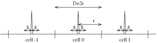
Figure 1: Infinite linear array cellular model.

Consider a wireless cellular system with $K$ user terminals (UTs) per cell where all users share the same bandwidth and Base Stations (BSs) are arranged on a uniform grid on a line (see Fig. 1). This model was pioneered by Wyner in [1] under a very simplified channel gain assumption, where the path gain to the closest BS is 1, the path gain to adjacent BSs is $\alpha$ and it is zero elsewhere. Wyner considered optimal joint processing of all base stations. Later, Shamai and Wyner [2] considered a similar model with frequency flat fading and more conventional decoding schemes, ranging from the standard separated base station processing to some forms of limited cooperation. A very large literature followed and extended these works in various ways (see for example [3, 4]).

In this paper we focus on the uplink of a conventional system, such that each BS decodes only the users in its own cell and treats inter-cell interference as noise. We extend the model in two directions: 1) we consider realistic propagation channels determined by a position-dependent path loss, and by a slowly time-varying frequency-selective fading channel; 2) we compare the optimal isolated cell delay-limited scheme [5] with the Proportional Fair Scheduling (PFS) scheme [6, 7].

In a delay-limited scheme each user transmits at a fixed rate in each fading block, and the system uses power control in order to cope with the time-varying channel conditions [5]. A delay-limited system achieves “hard fairness” (HF), in the sense that each user transmits at its own desired rate, independently of the fading channel realization. On the other hand, generally higher throughput can be achieved by relaxing the fixed rate per slot constraint. Under variable rate allocation, the sum throughput is maximized by letting only the user with the best channel transmit in each slot [8]. However, if users are affected by different distance-dependent path losses that change on a time-scale much slower than the small scale fading, this strategy may result in a very unfair resource allocation. In this case, PFS achieves a desirable tradeoff, by maximizing the geometric mean of the long-term average throughputs of the users [7].

HF and PFS have been compared in terms of system throughput versus $E_{b}/N_{0}$ in [9] for the single-cell case. This comparison is indeed relevant: HF models how voice-based systems work today and how Quality-of-Service guaranteed systems will work in the future (each user makes a rate request and the system struggles to accommodate it). In contrast, PFS is being implemented in the so-called EV-DO 3rd generation systems [6] in order to take advantage of delay-tolerant data traffic. Hence, a meaningful question is: what system capacity loss is to be expected by imposing hard-fairness? In this paper we address this question by extending the results of [9] to the multicell case with conventional decoding (i.e., without joint processing of the BSs).

II System Model

Each cell experiences interference from the signals transmitted by UTs in other cells. Frequency-selectivity is modeled by considering $M$ parallel frequency-flat subchannels. Roughly speaking, we may identify $M$ with the number of fading coherence bandwidths in the system signal bandwidth [10, 11, 12]. The received signal at BS $n$ in subchannel $m$ is given by

$$r^{m}(n)=\sum_{j=-\infty}^{\infty}\sum_{k=1}^{K}h_{k}^{m}(n,j)x_{k}^{m}(j)+z^{m}(n)$$ (1)

where $h_{k}^{m}(n,j)$ denotes the $m$-th subchannel gain from user $k$ at cell $j$ to cell $n$, and $x_{k}^{m}(j)$ denotes the signal of $m$-th subchannel transmitted by user $k$ in cell $j$, and $z^{m}(n)$ is an additive white Gaussian noise with variance $N_{0}$. The channel (power) gain is given by $g_{k}^{m}(n,j)=|h_{k}^{m}(n,j)|^{2}$ and the transmit power of a user is given by $\mbox{\bb E}[|x_{k}^{m}(j)|^{2}]=E_{k}^{m}(j)$.

We model the channel gain as the product of two terms, $g_{k}^{m}(n,j)=s_{k}(n,j)f_{k}^{m}(n,j)$, where $s_{k}(n,j)$ denotes a frequency-flat path gain that depends on the distance between the BS and the UT, and $f_{k}^{m}(n,j)$ is a “small-scale” fading term that depends on local scattering environment around user terminal [12]. These two components are mutually independent as they are due to different propagation effects. Path loss takes the expression $s_{k}(n,j)=d_{k}(n,j)^{-\alpha}$, where $d_{k}(n,j)$ denotes the the distance from base station $n$ to user $k$ in cell $j$ and $\alpha$ is the path loss exponent. We assume that UTs are not located in a forbidden region at distance less than $\delta$ from the BS so that the path loss does not diverge. When the users are uniformly distributed in each cell, the cdf of $s\equiv s_{k}(n,n)$ is given by

$$F_{s}(x)=\left\{\begin{array}[]{ll}0,&x<r^{-\alpha}\\ 1-\frac{x^{-\frac{1}{\alpha}}-\delta}{r-\delta},&r^{-\alpha}\leq x<\delta^{-\alpha}\\ 1,&x\geq\delta^{-\alpha}\end{array}\right.$$ (2)

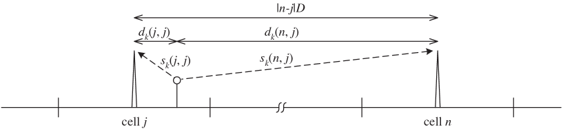
(a)

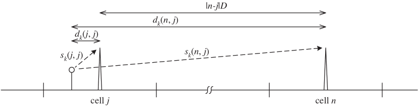
(b)

Figure 2: The path loss $s_{k}(n,j)$ that is determined by $s_{k}(j,j)$ in two ways.

where the cell radius is $r$ and the minimum distance between BSs is $D=2r$. The distance $d_{k}(n,j)$, $n\neq j$, is given by $d_{k}(n,j)=|n-j|D-d_{k}(j,j)$ or $d_{k}(n,j)=|n-j|D+d_{k}(j,j),$ depending on the location of user $k$ in cell $j$ as shown in Fig. 2. Consequently, the path loss $s_{k}(n,j)$ can be expressed as

$$s_{k}(n,j)=\theta_{k}(n,j)\left(|n-j|D-s_{k}(j,j)^{-\frac{1}{\alpha}}\right)^{-\alpha}+(1-\theta_{k}(n,j))\left(|n-j|D+s_{k}(j,j)^{-\frac{1}{\alpha}}\right)^{-\alpha},$$ (3)

where $\theta_{k}(n,j)$ takes on values 0 or 1 with equal probability since the UTs are distributed uniformly in each cell. We assume that the path losses change in time on a very slow scale, and can be considered as random, but constant, over the whole duration of transmission. In contrast, the small-scale fading changes relatively rapidly, even for moderately mobile users [10]. We assume Rayleigh block-fading, changing in an ergodic stationary manner from block to block, i.i.d., on the $M$ subchannels, $F_{f}(x)=1-e^{-x}$.

As in [2], we assume that all users send independently generated Gaussian random codes. Let $R_{k}^{m}(n)$ denote the rate per symbol allocated by user $k$ in cell $n$ on subchannel $m$. When outer-cell interference is akin Gaussian noise, the uplink capacity region of cell $n$ for fixed channel gains is given by the set of inequalities

$$\sum_{k\in S}R_{k}^{m}(n)\leq\log\left(1+\frac{\sum_{k\in S}g_{k}^{m}(n,n)E_{k}^{m}(n)}{N_{0}+I^{m}(n)}\right)$$ (4)

for all $S\subseteq\{1,2,\cdots,K\}$, where the interference at cell $n$ on subchannel $m$ is given by

$$I^{m}(n)=\sum_{j\neq n}\sum_{k=1}^{K}g_{k}^{m}(n,j)E_{k}^{m}(j).$$ (5)

The capacity region of the $M$ parallel channel case can be achieved by splitting each user information into $M$ parallel streams and sending the independent codewords over parallel channels. The aggregate rate of user $k$ at cell $n$ is given by

$$R_{k}(n)=\sum_{m=1}^{M}R_{k}^{m}(n),~{}~{}~{}k=1,2,\cdots,K.$$ (6)

II-A Delay-Limited Systems

In a delay-limited system, the rates $R_{k}(n)$ are fixed a priori, and the system allocates the transmit energies in order such that the rate $K$-tuple $(R_{1}(n),\cdots,R_{K}(n))$ is inside the achievable region in each fading block [5, 9]. We define the system $E_{b}/N_{0}$ under a coding strategy that supports user rates $(R_{1}(n),\cdots,R_{K}(n))$ as

$$\left(\frac{E_{b}}{N_{0}}\right)_{\rm sys}=\frac{1}{N_{0}\Gamma}\sum_{k=1}^{K}\sum_{m=1}^{M}E_{k}^{m}(n),$$ (7)

where the total number of bits per cell, $\Gamma$, is given by $\Gamma=\sum_{k=1}^{K}R_{k}(n)$. The system spectral efficiency C is given by $\textsf{C}=\frac{\Gamma}{M}$ and it is expressed in bits per second per hertz (bit/s/Hz) or, equivalently, in bits per dimension.

For given user rates $(R_{1}(n),\cdots,R_{K}(n))$, we allocate the partial rates $R_{k}^{m}(n)$ under the constraints (6) in order to minimize $(E_{b}/N_{0})_{\rm sys}$. As a subproblem for this optimization problem, we first consider the $m$-th subchannel energy allocation assuming that the partial rates and the interference $I^{m}(n)$ are given. Thanks to the fact that the received energy region is a contra-polymatrid [5], the optimal energy allocation is given explicitly as

$$E_{\pi_{k}^{m}(n)}^{m}(n)=\frac{N_{0}+I^{m}(n)}{g_{\pi_{k}^{m}(n)}^{m}(n,n)}\left[\exp\left(\sum_{i\leq k}R_{\pi_{i}^{m}(n)}^{m}(n)\right)-\exp\left(\sum_{i<k}R_{\pi_{i}^{m}(n)}^{m}(n)\right)\right],$$ (8)

where $\pi^{m}(n)$ is the permutation of $\{1,2,\cdots,K\}$ that sorts the channel gains in increasing order, i.e., $g_{\pi_{1}^{m}(n)}^{m}(n,n)\leq\cdots\leq g_{\pi_{K}^{m}(n)}^{m}(n,n)$ and the decoding order at base station $n$ is given by $\pi_{K}^{m}(n)$ (decoded first), $\pi_{K-1}^{m}(n),\cdots,\pi_{1}^{m}(n)$ (decoded last).

Since the energy allocation in (8) is the minimum sum energy allocation for given partial rates, it remains to minimize the total energy by optimizing the partial rates under the constraints (6). Inserting (8) into (7), we obtain the optimization problem for minimum system $E_{b}/N_{0}$

$$\min\frac{1}{N_{0}\Gamma}\sum_{k=1}^{K}\sum_{m=1}^{M}\frac{N_{0}+I^{m}(n)}{g_{\pi_{k}^{m}(n)}^{m}(n,n)}\left[\exp\left(\sum_{i\leq k}R_{\pi_{i}^{m}(n)}^{m}(n)\right)-\exp\left(\sum_{i<k}R_{\pi_{i}^{m}(n)}^{m}(n)\right)\right]$$ (9)

under the constraints (6). The interference experienced by base station $n$ on subchannel $m$ takes on the expression

$$I^{m}(n)=\sum_{j\neq n}\sum_{k=1}^{K}g_{\pi_{k}^{m}(n)}^{m}(n,j)\frac{N_{0}+I^{m}(j)}{g_{\pi_{k}^{m}(j)}^{m}(j,j)}\left[\exp\left(\sum_{i\leq k}R_{\pi_{i}^{m}(j)}^{m}(j)\right)-\exp\left(\sum_{i<k}R_{\pi_{i}^{m}(j)}^{m}(j)\right)\right]$$ (10)

because the partial rate allocation is performed locally at each cell. An operating point $(\left(\frac{E_{b}}{N_{0}}\right)_{\rm sys},\textsf{C})$ on the power/spectral efficiency plane is a function of both the signaling strategy and the individual user rates as well as of the channel gain joint distribution.

II-B Delay-Tolerant Systems

In a delay-tolerant system, the user rates can be adapted according to their instantaneous channel condition to achieve higher throughput at the cost of increasing delay. We consider the constant power allocation and let $\rho=E_{tot}/N_{0}$ denote the transmit SNR in each slot. Note that the water-filling power allocation tends to the constant power allocation as SNR increases. We also assume that the channel gains are independent but not necessarily identically distributed across the users, and symmetrically distributed across the subchannels, that is, for any permutation $\pi$ of $\{1,2,\cdots,M\}$, the joint cumulative distribution function of channel gains satisfy $F(g_{k}^{1}(n,j),\cdots,g_{k}^{M}(n,j))=F(g_{k}^{\pi_{1}}(n,j),\cdots,g_{k}^{\pi_{M}}(n,j))$ for all $k$, $n$, $j$. This means that no subchannel is statistically worse or better than any other.

PFS allocates slots fairly among users in the case of a near-far situation [7]. The PFS algorithm serves user $k$ on subchannel $m$ in cell $n$ if $\hat{k}_{m}(n)=k$, where

$$\hat{k}_{m}(n)={\hbox{arg}}\max_{k^{\prime}=1,\cdots,K}\frac{1}{T_{k^{\prime}}(n)}\log\left(1+\frac{\rho g_{k^{\prime}}^{m}(n,n)}{1+\rho\sum_{j\neq n}g_{\hat{k}_{m}(j)}^{m}(n,j)}\right).$$ (11)

$\hat{k}_{m}(j)$ denotes the index of the user selected for transmission on $m$-th subchanel in cell $j$ by the PFS scheduling and $T_{k}(n)$ denotes the long-term average user throughput of user $k$ in cell $n$.

III Delay-Limited Systems for a Large Number of Users

The optimization problem (9) for fixed inter-cell interference is convex, but it does not yield a closed form solution. In order to gain insight into the problem we investigate the asymptotic case for $K\rightarrow\infty$, for which a closed form solution exists. We make the following assumptions:

• $M$ is fixed while $K$ becomes arbitrarily large.

• As $K\rightarrow\infty$, the empirical distributions of $s_{k}(n,n)$, $\{f_{k}^{m}(n,j):m=1,\ldots,M\}$ and of $\theta_{k}(n,j)$ converge almost surely to given deterministic cdfs, $F_{s}(x)$, $F_{f}(y_{1},\cdots,y_{M})$, and $F_{\theta}(\phi)$, respectively. The cdf $F_{f}(y_{1},\cdots,y_{M})$ is symmetric, with identical marginal cdfs $F_{f}(y)$. The cdf $F_{\theta}(\phi)$ has two mass points at 0 and $1$, with equal probability mass $1/2$.

• For a given system throughput $\Gamma$, the user individual rates are given by $R_{k}(n)=\frac{\Gamma}{K}\nu_{k}(n)$, where $\nu_{k}(n)$ is the rate allocation factor for user $k$ in cell $n$. As $K\rightarrow\infty$, the empirical rate distribution converges almost surely to a given deterministic cdf $F_{\nu}(\mu)$ with mean 1 and support in $[a,b]$, where $0\leq a\leq b<\infty$ are constants independent of $K$.

• The rate allocation factors are fixed a priori, independently of the realization of the channel gains. Therefore, the empirical joint distribution of $\{(s_{k}(n,n),f_{k}^{1}(n,j),\cdots,f_{k}^{M}(n,j),$ $\theta_{k}(n,j),\nu_{k}(n)):k=1,\cdots,K\}$ converges to the product cdf $F_{s}(x)F_{f}(y_{1},\cdots,y_{M})F_{\theta}(\phi)F_{\nu}(\mu)$.

III-A Asymptotic Performance

In the single cell case, the minimum $(E_{b}/N_{0})_{\rm sys}$ for given C is given by [9]

$$\left(\frac{E_{b}}{N_{0}}\right)_{\rm sys}^{\rm SC}=\log(2)\int 2^{\textsf{C}G_{M}(x)}\frac{dG_{M}(x)}{x}.$$ (12)

where $G_{M}(x)$ denotes the cdf of $s\max\{f^{1},\ldots,f^{M}\}$, where $s\sim F_{s}(x)$ and $(f^{1},\ldots,f^{M})\sim F_{f}(y_{1},\ldots,y_{M})$. For the infinite linear array cellular model, we establish the following result.

Theorem 1

Under the assumptions A1, A2, A3, and A4, as $K\rightarrow\infty$ the minimum $(E_{b}/N_{0})_{\rm sys}$ for given system spectral efficiency C in an infinite linear array cellular model is given by

$$\left(\frac{E_{b}}{N_{0}}\right)_{\rm sys}^{\rm MC}=\frac{\log(2)\int 2^{\textsf{C}G_{M}(x)}\frac{dG_{M}(x)}{x}}{1-\textsf{C}\log(2)\iint 2^{\textsf{C}G_{M}(xy)}\Phi(x)\frac{dF_{s}(x)dH_{M}(y)}{xy}}.$$ (13)

where $H_{M}(y)$ denotes the cdf of $\max\{f^{1},\ldots,f^{M}\}$ where $(f^{1},\ldots,f^{M})\sim F_{f}(y_{1},\ldots,y_{M})$, and where the function $\Phi(s)$ is given by

$$\Phi(x)=D^{-\alpha}\left(\zeta\left(\alpha,1-\frac{x^{-1/\alpha}}{D}\right)+\zeta\left(\alpha,1+\frac{x^{-1/\alpha}}{D}\right)\right),$$ (14)

where $\zeta(a,x)$ is the Riemann zeta function [15]. The minimum $(E_{b}/N_{0})_{\rm sys}$ is achieved by letting each user transmit on its best subchannel only, and by using superposition coding and successive decoding on each subchannel.

Proof:

See Appendix A. ∎

If we compare (13) with (12), we can observe three facts: First, $(E_{b}/N_{0})_{\rm sys}^{\rm MC}$ is higher than $(E_{b}/N_{0})_{\rm sys}^{\rm SC}$ for all C. So, for the multiple cell case, the higher $(E_{b}/N_{0})_{\rm sys}$ is required to achieve the same system spectral efficiency C due to intercell interference. Second, $(E_{b}/N_{0})_{\rm sys}^{\rm MC}$ converges to $(E_{b}/N_{0})_{\rm sys}^{\rm SC}$, as $\textsf{C}\rightarrow 0$. For low spectral efficiency, low transmit energy causes negligible interference to other cells, which effectively turns the multiple cell case into the single cell (interference-free) case. Third, there exists a spectral efficiency limit in the multiple cell case because $(E_{b}/N_{0})_{\rm sys}^{\rm SC}$ tends to infinity as $\textsf{C}\rightarrow\textsf{C}_{0}$, where $\textsf{C}_{0}$ is the root of the denominator of the right hand side in (13)

$$1-\textsf{C}_{0}\log(2)\iint 2^{\textsf{C}_{0}G_{M}(xy)}\Phi(x)\frac{dF_{s}(x)dH_{M}(y)}{xy}=0.$$ (15)

Any spectral efficiency can be supported in the single cell case as long as the transmit energy is high. However, in the multiple cell case, high transmit energy to support high spectral efficiency may cause significant interference to other cells, thus demanding more transmit energy to combat interference from other cells. Eventually, additional energy to combat interference becomes tremendously large even in a finite spectral efficiency. So, the multiple cell case is an interference-limited system due to this fundamental spectral efficiency limit.

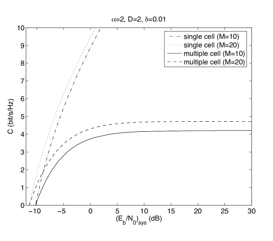
Figure 3: Spectral efficiency versus system $E_{b}/N_{0}$ for the optimal delay-limited systems for $K=\infty$. The channel parameters are $M=10$, the path loss exponent $\alpha=2$, the cell size $D=2$, and the forbidden region $\delta=0.01$.

Fig. 3 shows the spectral efficiency achieved by the delay-limited systems for infinite number of users and we can confirm the three properties described above. The spectral efficiency limits for $M=10$ and $M=20$ are $\textsf{C}_{0}=4.2$ bits/s/Hz and $\textsf{C}_{0}=4.73$ bits/s/Hz, respectively.

III-B Asymptotic Results for Simplified Multiple Cell Model

A well-known approach to the computation of system capacity of a conventional multi-cell system consists of modeling the inter-cell interference power as proportional to the total transmit power in each cell [13]. In this section we validate this approach and compute explicitly the proportionality constant. Let the interference level experienced by each cell be given by

$$I^{m}=\beta\sum_{k=1}^{K}E_{k}^{m}.$$ (16)

where we drop the cell index $n$ for simplicity. In (16), the ratio of interference and total transmit power is given by $\beta$. The capacity region of cell $n$ for cell-site optimal joint decoding is given by

$$\sum_{k\in S}R_{k}^{m}\leq\log\left(1+\frac{\sum_{k\in S}g_{k}^{m}E_{k}^{m}}{N_{0}+I^{m}}\right)$$ (17)

for all $S\subseteq\{1,2,\cdots,K\}$. For given $I^{m}$, the minimum total energy supporting a given rate ${\bf R}^{m}=(R_{1}^{m},\cdots,R_{K}^{m})$ with gains ${\bf g}^{m}=(g_{1}^{m},\cdots,g_{K}^{m})$ is given by

$$E_{\pi_{k}^{m}}^{m}=\frac{N_{0}+I^{m}}{g_{\pi_{k}^{m}}^{m}}\left[\exp\left(\sum_{i\leq k}R_{\pi_{i}^{m}}^{m}\right)-\exp\left(\sum_{i<k}R_{\pi_{i}^{m}}^{m}\right)\right],$$ (18)

where, as before, $\pi^{m}$ is sorting permutation of the channel gains in increasing order. We have:

Theorem 2

Under the assumptions A1, A2, A3, and A4, as $K\rightarrow\infty$ the minimum $(E_{b}/N_{0})_{\rm sys}$ for given system spectral efficiency C in a simple multiple cell model is given by

$$\left(\frac{E_{b}}{N_{0}}\right)_{\rm sys}^{\rm MC}=\frac{\log(2)\int 2^{\textsf{C}G_{M}(x)}\frac{dG_{M}(x)}{x}}{1-\beta\textsf{C}\log(2)\int 2^{\textsf{C}G_{M}(x)}\frac{dG_{M}(x)}{x}}$$ (19)

The minimum $(E_{b}/N_{0})_{\rm sys}$ is achieved by letting each user transmit on its best subchannel only, and by using superposition coding and successive decoding on each subchannel.

Proof:

See Appendix C. ∎

By equating (13) and (19), we can solve for $\beta$ and obtain

$$\beta=\frac{\iint 2^{\textsf{C}G_{M}(xy)}\Phi(x)\frac{dF_{s}(x)dH_{M}(y)}{xy}}{\int 2^{\textsf{C}G_{M}(x)}\frac{dG_{M}(x)}{x}}.$$ (20)

Since $\zeta(a,1-x)+\zeta(a,1+x)$ is an increasing function of $x$ and $0\leq s^{-1/\alpha}/D\leq 1/2$, we have

$$2D^{-\alpha}\zeta(\alpha,1)\leq\beta\leq D^{-\alpha}(\zeta(\alpha,1/2)+\zeta(\alpha,3/2)).$$ (21)

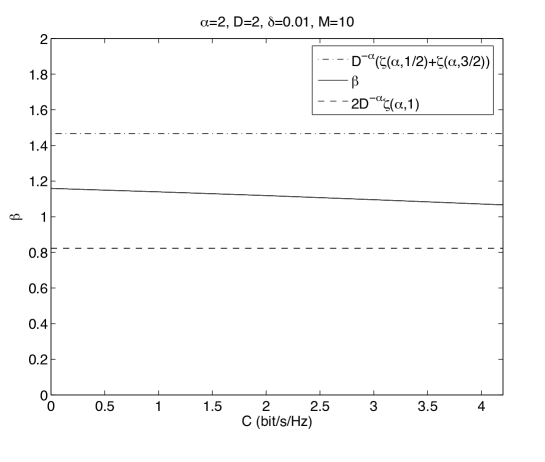
Figure 4: Power fraction $\beta$ and its upper and lower bounds for the optimal delay-limited systems for $K=\infty$. The channel parameters are path loss exponent $\alpha=2$, the cell size $D=2$, and the forbidden region $\delta=0.01$.

For example, if $\alpha=2$, then $3.29D^{-2}\leq\beta\leq 5.87D^{-2}$. This implies that there exists $\beta$ in $[2D^{-\alpha}\zeta(\alpha,1),D^{-\alpha}(\zeta(\alpha,1/2)+\zeta(\alpha,3/2))]$ such that the simple multiple cell model yields a valid result as in the infinite linear array cellular model. Fig. 4 shows $\beta$ in (20) and its upper and lower bounds in (21) for $M=10$, path loss exponent $\alpha=2$, the cell size $D=2$, and the forbidden region $\delta=0.01$. We observe that $\beta$ changes very little with respect to the spectral efficiency C. Hence, assuming $\beta$ constant as commonly done in simplified multicell analysis [13] yields good approximations.

We can rewrite the minimum $(E_{b}/N_{0})_{\rm sys}^{\rm MC}$ in terms of $(E_{b}/N_{0})_{\rm sys}^{\rm SC}$

$$\left(\frac{E_{b}}{N_{0}}\right)_{\rm sys}^{\rm MC}=\frac{\left(\frac{E_{b}}{N_{0}}\right)_{\rm sys}^{\rm SC}}{1-\beta\textsf{C}\left(\frac{E_{b}}{N_{0}}\right)_{\rm sys}^{\rm SC}}.$$ (22)

So, the performance degradation due to the multiple cell interference is up to 3 dB as long as

$$\left(\frac{E_{b}}{N_{0}}\right)_{\rm sys}^{\rm SC}\leq\frac{1}{2\beta\textsf{C}}.$$ (23)

In the case when the interference dominates the noise, the performance degradation is more than 3 dB and the $(E_{b}/N_{0})_{\rm sys}^{\rm MC}$ tends to infinity as $\textsf{C}\rightarrow\textsf{C}_{0}$. We may summarize the conditions that determine the performance of the multiple cell case

$$\left\{\begin{array}[]{cl}\left(\frac{E_{b}}{N_{0}}\right)_{\rm sys}^{\rm SC}\leq\frac{1}{2\beta\textsf{C}},&\mbox{noise dominated region}\\ \frac{1}{2\beta\textsf{C}}<\left(\frac{E_{b}}{N_{0}}\right)_{\rm sys}^{\rm SC}<\frac{1}{\beta\textsf{C}},&\mbox{interference dominated region}\\ \left(\frac{E_{b}}{N_{0}}\right)_{\rm sys}^{\rm SC}\geq\frac{1}{\beta\textsf{C}},&\mbox{forbidden region}\end{array}\right.$$ (27)

For $\textsf{C}=2.8$ bit/s/Hz, $\left(\frac{E_{b}}{N_{0}}\right)_{\rm sys}^{\rm SC}=-7.967$ dB and $\frac{1}{2\beta\textsf{C}}=-7.896$ dB when $\beta\simeq 1.1$ (see Fig. 4). According to (27), the system may be regarded as operated in the noise-dominated region because $\left(\frac{E_{b}}{N_{0}}\right)_{\rm sys}^{\rm SC}<\frac{1}{2\beta\textsf{C}}$. We can verify this by checking $\left(\frac{E_{b}}{N_{0}}\right)_{\rm sys}^{\rm MC}=-5.024$ dB in Fig. 3. So, as long as the target spectral efficiency is less than 2.8 bit/s/Hz, additionally required energy in the multiple cell is no more than 3 dB compared to the single cell. It should also be noticed that practical systems nowadays achieve spectral efficiencies of about 1 bit/s/Hz. It follows that, in practice, there is still a significant gap before the interference-limited nature of the multicell system becomes significant. Therefore, implementing some clever low complexity separated cell-site processing may not be a bad idea from the practical system engineering viewpoint. For example, using successive decoding at each BS, as the system analyzed in this paper, represents already a remarkable step-forward with respect to orthogonal or semi-orthogonal conventional techniques such as TDMA, FDMA, CDMA, OFDM or a mixture thereof.

III-C Partial Reuse Transmission

In order to alleviate the interference limited nature of the multi-cell delay-limited system, we introduce a partial reuse transmission scheme. We notice here that in the traditional Wyner cellular model non-adjacent do not interfere. Trivially, a reuse factor of 2 (even-odd cells) yields a non-interference limited system [2]. With a more realistic distance-dependent path loss model as in our case, this is no longer true and reuse factor optimization becomes more delicate.

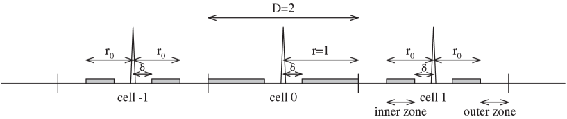
(a)

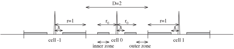
(b)

Figure 5: Cellular model for partial reuse transmission in which users located in shaded areas are only allowed to transmit signals in (a) phase 1 and (b) phase 2.

Without loss of generality we can set the cell size $D=2$ (generalization is trivially obtained by cell re-scaling). Fig. 5 shows the system model for partial reuse transmission. We classify cells into even and odd groups, according to their index parity. We also divide each cell into an inner and outer regions, where the inner region radius is $\delta\leq r_{0}\leq 1$. The users located in the inner zone transmit in each slot. Users located in the outer zone transmit signals alternately, at even slot times if they belong to an even cell, or odd slot times if they belong to an odd cell. Consequently, the activity duty cycle of the users located in the outer zone is 0.5.

From (2), the cdf of the path loss when users are uniformly distributed in $(a,b)$ is given by

$$F_{s}^{(a,b)}(x)=\left\{\begin{array}[]{ll}0,&x<b^{-\alpha}\\ 1-\frac{x^{-\frac{1}{\alpha}}-a}{b-a},&b^{-\alpha}\leq x<a^{-\alpha}\\ 1,&x\geq a^{-\alpha}\end{array}.\right.$$ (28)

Due to the symmetry, it suffices to focus only on the phase where even cells are fully active. In this case, the active users in odd cells are uniformly distributed in $(\delta,r_{0})$ while the users in even cells are uniformly distributed in $(\delta,1)$. Letting $K_{0}=K$ denote the number of active users in even cells, the number of active users in odd cells is $K_{1}=\frac{r_{0}-\delta}{1-\delta}K$. Similarly, we set the number of bits transmitted in each odd cell is $\Gamma_{1}=\frac{r_{0}-\delta}{1-\delta}\Gamma_{0}$ when the number of bits transmitted in each even cell is $\Gamma_{0}$. Based on these, the spectral efficiency in this partial reuse system is

$$\textsf{C}=\frac{\Gamma_{0}+\Gamma_{1}}{2M}=\frac{\Gamma_{0}}{2M}\frac{1+r_{0}-2\delta}{1-\delta}.$$ (29)

Also, the $(E_{b}/N_{0})_{\rm sys}$ is defined by

$$\left(\frac{E_{b}}{N_{0}}\right)_{\rm sys}=\frac{E_{\rm tot}^{0}+E_{\rm tot}^{1}}{N_{0}(\Gamma_{0}+\Gamma_{1})}=\frac{E_{\rm tot}^{0}+E_{\rm tot}^{1}}{2N_{0}M\textsf{C}},$$ (30)

where $E_{\rm tot}^{0}$ and $E_{\rm tot}^{1}$ denote the total transmitted energy in each even cell and each odd cell, respectively. We have:

Theorem 3

Under the assumptions A1, A2, A3, and A4, as $K\rightarrow\infty$, the minimum $(E_{b}/N_{0})_{\rm sys}$ for given system spectral efficiency C for the partial reuse system in an infinite linear array cellular model is given by

$$\left(\frac{E_{b}}{N_{0}}\right)_{\rm sys}^{\rm MC-Partial}=\frac{1}{2}\frac{1+A_{01}-A_{11}}{1-A_{00}-A_{11}-A_{01}A_{10}+A_{01}A_{11}}\frac{2(1-\delta)}{1+r_{0}-2\delta}$$

$$\cdot\log(2)\int 2^{\frac{2\textsf{C}(1-\delta)}{1+r_{0}-2\delta}G_{M}(x)}\frac{dG_{M}(x)}{x}~{}~{}$$

$$+\frac{1}{2}\frac{1+A_{10}-A_{00}}{1-A_{00}-A_{11}-A_{01}A_{10}+A_{01}A_{11}}\frac{2(r_{0}-\delta)}{1+r_{0}-2\delta}$$

$$\cdot\log(2)\int 2^{\frac{2\textsf{C}(r_{0}-\delta)}{1+r_{0}-2\delta}G_{M}^{(\delta,r_{0})}(x)}\frac{dG_{M}^{(\delta,r_{0})}(x)}{x}~{}.$$ (31)

Here $A_{ij}$’s are given by

$$A_{00}=\log(2)\frac{2\textsf{C}(1-\delta)}{1+r_{0}-2\delta}\iint 2^{\frac{2\textsf{C}(1-\delta)}{1+r_{0}-2\delta}G_{M}(xy)}\Phi_{0}(x)\frac{dF_{s}(x)dH_{M}(y)}{xy}~{}$$ (32a)

$$A_{01}=\log(2)\frac{2\textsf{C}(r_{0}-\delta)}{1+r_{0}-2\delta}\iint 2^{\frac{2\textsf{C}(r_{0}-\delta)}{1+r_{0}-2\delta}G_{M}^{(\delta,r_{0})}(xy)}\Phi_{1}(x)\frac{dF_{s}^{(\delta,r_{0})}(x)dH_{M}(y)}{xy}$$ (32b)

$$A_{10}=\log(2)\frac{2\textsf{C}(1-\delta)}{1+r_{0}-2\delta}\iint 2^{\frac{2\textsf{C}(1-\delta)}{1+r_{0}-2\delta}G_{M}(xy)}\Phi_{1}(x)\frac{dF_{s}(x)dH_{M}(y)}{xy}~{}$$ (32c)

$$A_{11}=\log(2)\frac{2\textsf{C}(r_{0}-\delta)}{1+r_{0}-2\delta}\iint 2^{\frac{2\textsf{C}(r_{0}-\delta)}{1+r_{0}-2\delta}G_{M}^{(\delta,r_{0})}(xy)}\Phi_{0}(x)\frac{dF_{s}^{(\delta,r_{0})}(x)dH_{M}(y)}{xy}$$ (32d)

where

$$\Phi_{0}(x)=4^{-\alpha}\left(\zeta\left(\alpha,1-\frac{x^{-1/\alpha}}{4}\right)+\zeta\left(\alpha,1+\frac{x^{-1/\alpha}}{4}\right)\right)~{}~{}$$ (33a)

$$\Phi_{1}(x)=4^{-\alpha}\left(\zeta\left(\alpha,\frac{1}{2}-\frac{x^{-1/\alpha}}{4}\right)+\zeta\left(\alpha,\frac{1}{2}+\frac{x^{-1/\alpha}}{4}\right)\right).$$ (33b)

Proof:

See Appendix D. ∎

In the expressions above, $G_{M}^{(\delta,r_{0})}(x)$ denotes the cdf of $s\max\{f^{1},\ldots,f^{M}\}$ when $s\sim F_{s}^{(\delta,r_{0})}(x)$ and $(f^{1},\ldots,f^{M})\sim F_{f}(y_{1},\ldots,y_{M})$. It can be readily checked that the case of $r_{0}=1$ coincides with the full reuse, that we have analyzed separately in Theorem 1. If $r_{0}=\delta$, then half of cells are silent to reduce interference, which corresponds to the reuse factor of 2, also referred to as intercell time division transmission system. We also notice that the performance of frequency reuse, i.e., partitioning the $M$ frequency subchannels into two subsets and allocate them to even and odd cells, cannot outperform the “time” reuse studied in Theorem 3 since the frequency diversity in each cell would be reduced. Of course, the reuse parameter $r_{0}$ may be optimized in order to minimize the required $(E_{b}/N_{0})_{\rm sys}$ for given spectral efficiency C.

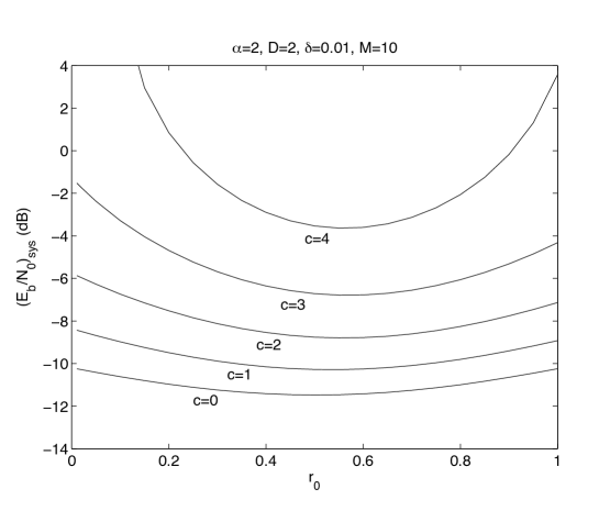
Figure 6: System $E_{b}/N_{0}$ versus $r_{0}$ for the delay-limited system in the partial reuse transmission scheme for $K=\infty$. The channel parameters are the path loss exponent $\alpha=2$, the cell size $D=2$, the forbidden region $\delta=0.01$, and $M=10$.

Fig. 6 depicts $(E_{b}/N_{0})_{\rm sys}^{\rm MC-Partial}$ in (31) versus $r_{0}$ for the partial reuse transmission system. There is an optimal $r_{0}\in(\delta,1]$ that minimizes $(E_{b}/N_{0})_{\rm sys}^{\rm MC-Partial}$ for given C. At $\textsf{C}=4$, the $(E_{b}/N_{0})_{\rm sys}$ difference between the full transmission and the optimal partial reuse transmission is about 7 dB, that is quite significant. This shows that large gains can be realized by careful optimization of the partial reuse factor.

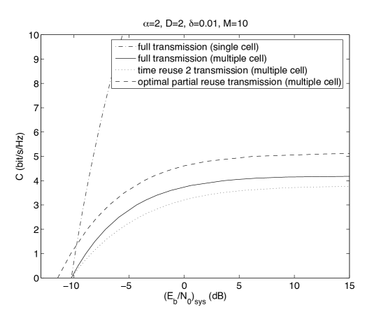
Figure 7: Spectral efficiency versus system $E_{b}/N_{0}$ for the delay-limited system in the optimal partial reuse transmission scheme for $K=\infty$. The channel parameters are the path loss exponent $\alpha=2$, the cell size $D=2$, the forbidden region $\delta=0.01$, and $M=10$.

Fig. 7 shows the optimal partial reuse transmission scheme compared with the full transmission schemes in the single and multiple cell cases and reuse 2 scheme in the multiple cell case. We notice here that the gain due to partial reuse comes at the expenses of relaxing slightly the HF constraint: users in the outer zone of each cell is half of their requested rate, since they are served with duty cycle 0.5. For this reason, in the regime of small C the multicell system with partial reuse outperforms the single-cell HF system.

IV Performance of Delay-Tolerant Systems

A delay-tolerant system can achieve high spectral efficiency at the cost of loose delay requirement. In a distance-dependent path-loss scenario as considered here, it can be shown that PFS serves user at the peak of its own small-scale fading, i.e., the path-loss takes no role in the channel allocation [9]. In this section, we investigate the performance of PFS in our multi-cell setting.

IV-A Spectral Efficiency Bounds

According to Theorem 1 in [9], in the case of the single cell, the spectral efficiency C as a function of $\left(\frac{E_{b}}{N_{0}}\right)_{\rm sys}$ is given implicitly by

$$\textsf{C}=\mbox{\bb E}\left[\log_{2}(1+\rho s\max_{k}f_{k})\right]$$

$$\left(\frac{E_{b}}{N_{0}}\right)_{\rm sys}^{\rm SC-PFS}=\frac{\rho}{\textsf{C}}~{}~{}~{}~{}~{}~{}~{}~{}~{}~{}~{}~{}~{}~{}~{}~{}~{}~{}~{}~{}~{}~{}~{}~{}~{}~{}~{}$$ (34)

where $s\sim F_{s}(x)$ given by (2) and $f_{k}$ is distributed as the frequency selective block fading of user $k$. Similarly, we have:

Theorem 4

For any given $K$, the spectral efficiency and the system $E_{b}/N_{0}$ achieved by the PFS are given by

$$\textsf{C}=\mbox{\bb E}\left[\log_{2}\left(1+\frac{\rho s\max_{k=1,2,\cdots,K}f_{k}}{1+\rho\sum_{j\neq n}g_{\hat{k}(j)}(n,j)}\right)\right]$$

$$\left(\frac{E_{b}}{N_{0}}\right)_{\rm sys}^{\rm MC-PFS}=\frac{\rho}{\textsf{C}}~{}~{}~{}~{}~{}~{}~{}~{}~{}~{}~{}~{}~{}~{}~{}~{}~{}~{}~{}~{}~{}~{}~{}~{}~{}~{}~{}~{}~{}~{}~{}~{}~{}~{}~{}~{}~{}~{}~{}~{}~{}~{}~{}~{}~{}$$ (35)

where $\hat{k}(j)$ is the index of the user selected for transmission in cell $j$.

Proof:

Because of the symmetry of the small-scale fading distribution, the average throughput for each subchannel is identical. So, it is sufficient to focus on a single subchannel and we drop the subchannel index $m$. Since each user in the same cell gets the same interference $I=\sum_{j\neq n}g_{\hat{k}(j)}(n,j)$ in (11), the PFS scheduling decision in the multiple cell is the same with that in the single cell if the noise is replaced with $1+\rho I$. From Theorem 1 in [9], the result follows straightforwardly. ∎

From (3), $g_{\hat{k}(j)}(n,j)$ can be expressed as

$$g_{\hat{k}(j)}(n,j)\sim\left(\theta(|n-j|D-U)^{-\alpha}+(1-\theta)(|n-j|D+U)^{-\alpha}\right)f(n,j),$$ (36)

where $U$ is a uniform random variable ranging from $\delta$ to $r$, $\theta$ is a binary random variable taking 0 or 1 with equal probability, and $f(n,j)$ is unit-mean exponentially distributed.

We can derive some bounds for the spectral efficiency as shown in Appendix E. The lower bound follows from Jensen’s inequality and is given by

$$\textsf{C}\geq\mbox{\bb E}\left[\log_{2}\left(1+\frac{\rho s\max_{k}f_{k}}{1+\rho I_{0}}\right)\right],$$ (37)

where the average interference is given by

$$I_{0}=\mbox{\bb E}\left[\sum_{j\neq n}g_{\hat{k}(j)}(n,j)\right]~{}~{}~{}~{}~{}~{}~{}~{}~{}~{}~{}~{}~{}~{}~{}~{}~{}~{}~{}~{}~{}~{}~{}~{}~{}~{}~{}~{}~{}~{}~{}~{}~{}~{}~{}~{}~{}~{}~{}~{}~{}~{}~{}~{}~{}~{}~{}~{}~{}~{}~{}~{}~{}~{}~{}~{}~{}~{}~{}~{}~{}~{}~{}~{}~{}$$

$$=\left\{\begin{array}[]{ll}\frac{1}{D(D/2-\delta)}\left(2-\frac{D}{\delta}+\pi\cot\left(\frac{\pi\delta}{D}\right)\right),&\mbox{if }\alpha=2\\ \frac{D^{-\alpha+1}}{(\alpha-1)(D/2-\delta)}\left(2^{\alpha-1}+\zeta\left(\alpha-1,1+\frac{\delta}{D}\right)-\zeta\left(\alpha-1,1-\frac{\delta}{D}\right)\right),&\mbox{if }\alpha\neq 2.\end{array}\right.$$ (40)

A simple upper bound is derived by considering the interference only from the two nearest cells

C $$\leq \mbox{\bb E}\left[\log_{2}\left(1+\rho s\max_{k}f_{k}+\rho I_{0}^{(2)}\right)\right]$$ (41)

$$-\mbox{\bb E}\left[\log_{2}\left(1+\rho(g_{\hat{k}(n-1)}(n,n-1)+g_{\hat{k}(n+1)}(n,n+1))\right)\right].$$

where the average interference is given by

$$I_{0}^{(2)}=\frac{D^{-\alpha+1}}{(\alpha-1)(D/2-\delta)}\left(2^{\alpha-1}-\left(\frac{2}{3}\right)^{\alpha-1}+\left(1+\frac{\delta}{D}\right)^{-\alpha+1}-\left(1-\frac{\delta}{D}\right)^{-\alpha+1}\right).$$ (42)

The proportional fairness system is also interference limited for any given finite $K$, because, as SNR increases, the spectral efficiency converges to a finite value

$$\textsf{C}_{0}=\lim_{\rho\rightarrow\infty}\textsf{C}=\mbox{\bb E}\left[\log_{2}\left(\frac{s\max_{k}f_{k}}{\sum_{j\neq n}g_{\hat{k}(j)}(n,j)}\right)\right].$$ (43)

However, under mild conditions on $f_{k}$ (e.g., they are independent and identically distributed (i.i.d.) exponential random variables), for $K\rightarrow\infty$ we have [14]

$$\Pr(|\max_{k}f_{k}-\log K|<\log\log K)\geq 1-O\left(\frac{1}{\log K}\right).$$ (44)

Consequently, the spectral efficiency limit $\textsf{C}_{0}$ is order of $O(\log\log K)$. Notice that the spectral efficiency of the delay-limited system converges to a finite value $\textsf{C}_{0}$ in (15) as $E_{b}/N_{0}\rightarrow\infty$, also in the case of $K\rightarrow\infty$. We conclude that the PFS delay-tolerant system has merit in terms of spectral efficiency limit because its spectral efficiency increases without bound as the number of users tends to infinity (another manifestation of the ubiquitous multiuser diversity principle).

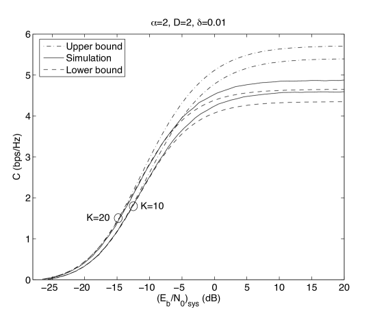
Figure 8: Spectral efficiency lower and upper bounds versus system $E_{b}/N_{0}$ for the proportional fair scheduling for $K=10$ and $K=20$. The channel parameters are path loss exponent $\alpha=2$, the cell size $D=2$, and the forbidden region $\delta=0.01$.

Fig. 8 shows the performance of PFS, the lower bound (37), and the upper bound (41). The lower bound is quite tight and the upper bound is close to the simulation result at low SNR regime. Compared to Fig. 3, we can observe that PFS generally outperforms the delay-limited system with infinite number of users in the regime of low to moderate SNR and yields similar throughput at high SNR.

V Conclusions

We provided a closed-form analysis of the system spectral efficiency vs. the system $E_{b}/N_{0}$ for two types of systems in a multi-cell “Wyner-like” cellular scenario, under the assumption of conventional single-BS processing. On one hand, we have a hard-fairness system where users transmit at fixed instantaneous rates in each slot and the system allocates power and makes use of successive interference cancellation decoding at each BS in order to minimize the required power to accommodate the user rate requests. On the other hand, we have a delay-tolerant system with variable instantaneous rate allocation in order to maximize the long-term system throughput subject to the proportional fairness constraint. Beyond the pleasant analytical details, the main outcomes of this work are: 1) We validated analytically the popular simplified multi-cell model that treats inter-cell interference power as proportional to the total cell power, evaluating the proportionality factor $\beta$ and showing that it is indeed close to a constant almost independent of spectral efficiency; 2) We showed that significant gains can be obtained by optimizing the partial reuse factor, letting users in the outer region of cells to transmit with duty-cycle 0.5; 3) We showed that PFS yields significant gains at low spectral efficiency, while for a finite number of users and high SNR the two systems are quite comparable. Hence, there is no silver bullet associated with PFS, and only a moderate increase in throughput over a hard-fairness system can be expected by exploiting the delay-tolerant nature of data traffic; 4) However, as $K$ increases, PSF yields an unbounded spectral efficiency while the HF system becomes interference limited. This is a manifestation of the multiuser diversity in a multi-cell environment.

Appendix A

Proof of Theorem 1

The proof is based on the proof of Theorem 2 in [9]. Let $R_{k}^{m}(n)=\frac{1}{K}\Gamma\nu_{k}^{m}(n)$, for all $k$ and $m$, be the partial rate allocation. We rewrite (9) for given interference $I^{m}(n)$ to minimize

$$\frac{1}{N_{0}\Gamma}\sum_{k=1}^{K}\sum_{m=1}^{M}\frac{N_{0}+I^{m}(n)}{g_{\pi_{k}^{m}(n)}^{m}(n)}\exp\left(\frac{\Gamma}{K}\sum_{i<k}\nu_{\pi_{i}^{m}(n)}^{m}(n)\right)\left(\exp\left(\frac{\Gamma}{K}\nu_{\pi_{k}^{m}(n)}^{m}(n)\right)-1\right)$$ (45)

subject to $\sum_{m=1}^{M}\nu_{k}^{m}(n)=\nu_{k}(n)$, $k=1,2,\cdots,K$, and to the non-negative constraints $\nu_{k}^{m}(n)\geq 0$ for all $k$ and $m$. Since $\exp(x)=1+x+o(x)$ for small $x$, the objective function for large $K$ can be written as

$$\frac{1}{N_{0}}\frac{1}{K}\sum_{k=1}^{K}\sum_{m=1}^{M}(N_{0}+I^{m}(n))\frac{\nu_{\pi_{k}^{m}(n)}^{m}(n)}{g_{\pi_{k}^{m}(n)}^{m}(n)}\exp\left(\frac{\Gamma}{K}\sum_{i<k}\nu_{\pi_{i}^{m}(n)}^{m}(n)\right)$$ (46)

and its associated Lagrangian function is

$$\mathcal{L}=\frac{1}{N_{0}}\frac{1}{K}\sum_{k=1}^{K}\sum_{m=1}^{M}\frac{\nu_{\pi_{k}^{m}(n)}^{m}(n)}{d_{\pi_{k}^{m}(n)}^{m}(n)}\exp\left(\frac{\Gamma}{K}\sum_{i<k}\nu_{\pi_{i}^{m}(n)}^{m}(n)\right)-\sum_{k=1}^{K}\lambda_{k}^{(K)}\left(\sum_{m=1}^{M}\nu_{k}^{m}-\nu_{k}\right),$$ (47)

where the channel SINR (signal to interference plus noise ratio) $d_{\pi_{k}^{m}(n)}^{m}(n)$ is given by $d_{\pi_{k}^{m}(n)}^{m}(n)\equiv g_{\pi_{k}^{m}(n)}^{m}(n)/(N_{0}+I^{m}(n))$. We have an optimization problem for each $K$ and $\lambda_{k}^{(K)}$ denotes the $k$th Lagrangian multiplier of the problem. By differentiating with respect to $\nu_{k}^{m}$, and by letting $\pi_{i}^{m}=k$, i.e., user $k$ is ranked in the $i$th position on subchannel $m$, the Kuhn-Tucker condition becomes

$$\frac{1}{d_{k}^{m}(n)}\exp\left(\frac{\Gamma}{K}\sum_{l<i}\nu_{\pi_{l}^{m}(n)}^{m}(n)\right)+\frac{\Gamma}{K}\sum_{l>i}\frac{\nu_{\pi_{l}^{m}(n)}^{m}(n)}{d_{\pi_{l}^{m}(n)}^{m}(n)}\exp\left(\frac{\Gamma}{K}\sum_{l^{\prime}<l}\nu_{\pi_{l^{\prime}}^{m}(n)}^{m}(n)\right)\geq\lambda_{k}^{(K)},$$ (48)

where we have multiplied both sides by $KN_{0}$ and have replaced $KN_{0}\lambda_{k}^{(K)}$ by $\lambda_{k}^{(K)}$. At this point, we notice that (48) coincides with the Kuhn-Tucker condition for the single cell case (see proof of Theorem 2 in [9]) provided that SNR [9] is replaced by the SINR $g_{\pi_{k}^{m}(n)}^{m}(n)/(N_{0}+I^{m}(n))$. Consequently, the asymptotically optimal rate allocation for large $K$ is given by [9]

$$\nu_{k}^{m}(n)=\left\{\begin{array}[]{cc}\nu_{k}(n),&\mbox{for}~{}m=m_{k}\\ 0,&\mbox{for}~{}m\neq m_{k}\end{array}\right.$$ (49)

where $m_{k}={\hbox{arg}}\max_{l}\{g_{k}^{l}(n,n)/(N_{0}+I^{m}(n))\}$ denotes the index of the subchannel for which user $k$ has maximum SINR. As a byproduct, we have that allocating each user to its own best SINR channel is asymptotically optimal for large $K$ in the multiple cell case. Since the subchannel distribution is symmetric and users are distributed uniformly in each cell, the interference $I^{m}(n)$ converges to the same non-random limit for all $m$ and $n$ as $K\rightarrow\infty$. If the interference is the same, then the optimal rate allocation for the multiple cell consists of allocating each user on its best SNR channel, i.e., $m_{k}={\hbox{arg}}\max_{l}\{g_{k}^{l}(n,n)\}$.

Now we show that allocating each user on its subchannel with best channel gain makes indeed the interference $I^{m}(n)$ constant with $m$ (constant with the cell index $n$ follows immediately form the symmetry of the system). From (10), for large $K$, the interference power is expressed as

$$I^{m}(n)=\sum_{j\neq n}(N_{0}+I^{m}(j))\frac{\Gamma}{K}\sum_{k=1}^{K}\frac{g_{\pi_{k}^{m}(n)}^{m}(n,j)\nu_{\pi_{k}^{m}(j)}^{m}(j)}{g_{\pi_{k}^{m}(j)}^{m}(j,j)}\exp\left(\frac{\Gamma}{K}\sum_{i<k}\nu_{\pi_{i}^{m}(j)}^{m}(j)\right)+o(1/K).$$ (50)

As we adopt an optimal successive decoding scheme in each BS, $\nu_{k}^{m}(j)$ takes the form in (49). Suppose that $g_{k}^{m}(j,j)$, given by $s_{k}(j,j)=x$ and $f_{k}^{m}(j,j)=y$, is ranked in the $i$th position by the permutation $\pi^{m}(j)$. By using Lemma 1 in Appendix B, we get

$$\exp\left(\frac{\Gamma}{K}\sum_{i<k}\nu_{\pi_{i}^{m}(j)}^{m}(j)\right)\rightarrow\exp\left(\frac{\Gamma}{M}G_{M}(xy)\right)$$ (51)

as $K\rightarrow\infty$. From (3), averaging with respect to $\theta_{k}(n,j)$, we get

$$\mbox{\bb E}\left[s_{k}(n,j)|s_{k}(j,j)\right]=\frac{1}{2}\left(\left(|n-j|D-s_{k}(j,j)^{-\frac{1}{\alpha}}\right)^{-\alpha}+\left(|n-j|D+s_{k}(j,j)^{-\frac{1}{\alpha}}\right)^{-\alpha}\right)$$ (52)

According to Lemma 2 in Appendix B, the asymptotic interference in (50) for large $K$ becomes

$$I^{m}(n)=\sum_{j\neq n}(N_{0}+I^{m}(j))\frac{\Gamma}{M}\iint e^{\frac{\Gamma}{M}G_{M}(xy)}\Phi(x,|n-j|D)\frac{dF_{s}(x)dH_{M}(y)}{xy},~{}$$ (53)

where $\Phi(x,y)\equiv\frac{1}{2}\left(\left(y-x^{-\frac{1}{\alpha}}\right)^{-\alpha}+\left(y+x^{-\frac{1}{\alpha}}\right)^{-\alpha}\right)$. Note that the interference relation in (53) is symmetric with respect to $I^{m}(n)$ for all $m$ and $n$. Therefore, as $K\rightarrow\infty$, the interference at each base station converges to the same value, $I^{m}(n)\rightarrow I_{0}$, for all $m$ and $n$. As $I^{m}(n)\rightarrow I_{0}$, we have

$$I_{0}=(N_{0}+I_{0})\frac{\Gamma}{M}\iint e^{\frac{\Gamma}{M}G_{M}(xy)}\Phi(x)\frac{dF_{s}(x)dH_{M}(y)}{xy},$$ (54)

where $\Phi(x)\equiv 2\sum_{j=1}^{\infty}\Phi(x,jD)$. Solving (54) with respect to $I_{0}$, we obtain the asymptotic interference under the single-cell optimal successive decoding strategy. In addition, by Lemma 1 in Appendix B, allocating each user on its own best channel makes the minimum $(E_{b}/N_{0})_{\rm sys}$ in (46) converges to the following

$$\left(\frac{E_{b}}{N_{0}}\right)_{\rm sys}\rightarrow\frac{N_{0}+I_{0}}{N_{0}}\int_{0}^{\infty}\frac{1}{x}\exp\left(\frac{\Gamma}{M}G_{M}(x)\right)dG_{M}(x)$$ (55)

as $K\rightarrow\infty$ (again, this can be easily shown based on the proof of Theorem 2 in [9]). Inserting the expression of $I_{0}$ from (54) into (55) and expressing $\Gamma$ in bits, we eventually arrive at the desired result.

Appendix B

Lemmas

Lemma 1

[9] Let A be an interval, and $\textsl{A}(m)$ denote the set

$$\textsl{A}(m)=\left\{k|s_{k}(n,n)\max\{f_{k}^{1}(n,n),\cdots,f_{k}^{M}(n,n)\}\in\textsl{A},m_{k}=m\right\},$$ (56)

where $m_{k}\equiv{\hbox{arg}}\max_{l}\{f_{k}^{l}(n,n)\}$. Also, let $g(x)$ denote a continuous measurable function in $x\in A$. Under Assumptions A2, A3, and A4, we get

$$\frac{1}{K}\sum_{k\in\textsl{A}(m)}g(s_{k}(n,n)f_{k}^{m}(n,n))\nu_{k}\rightarrow\frac{1}{M}\int_{x\in\textsl{A}}g(x)dG_{M}(x)$$ (57)

with probability 1, as $K\rightarrow\infty$ and $M$ is fixed.

Lemma 2

Let A be an interval, and $\textsl{A}(m)$ denote the set

$$\textsl{A}(m)=\left\{k|s_{k}(j,j)\max\{f_{k}^{1}(j,j),\cdots,f_{k}^{M}(j,j)\}\in\textsl{A},m_{k}=m\right\},$$ (58)

where $m_{k}\equiv{\hbox{arg}}\max_{l}\{f_{k}^{l}(j,j)\}$. Also, let $g(x,\phi)$ denote a continuous measurable function in $x\in A$ and $\phi\geq 0$. Under Assumptions A2, A3, and A4, we get

$$\frac{1}{K}\sum_{k\in\textsl{A}(m)}\frac{g(s_{k}(j,j),\theta_{k}(n,j))f_{k}^{m}(n,j)\nu_{k}}{s_{k}(j,j)f_{k}^{m}(j,j)}\rightarrow\frac{1}{M}\iint_{xy\in\textsl{A}}\frac{\mbox{\bb E}_{\theta}[g(x,\theta)]}{xy}dF_{s}(x)dH_{M}(y)$$ (59)

with probability 1, as $K\rightarrow\infty$ and $M$ is fixed. In (59), $\mbox{\bb E}_{\theta}[\cdot]$ denotes expectation with respect to $\theta\sim F_{\theta}(\phi)$.

Proof:

It follows from the convergence of the empirical cdfs that, as $K\rightarrow\infty$, we have

$$\frac{1}{K}\sum_{k\in\textsl{A}(m)}\frac{g(s_{k}(j,j),\theta_{k}(n,j))f_{k}^{m}(n,j)\nu_{k}}{s_{k}(j,j)f_{k}^{m}(j,j)}~{}~{}~{}~{}~{}~{}~{}~{}~{}~{}~{}~{}~{}~{}~{}~{}~{}~{}~{}~{}~{}~{}~{}~{}~{}~{}$$

$$=\frac{|\textsl{A}(m)|}{K}\frac{1}{|\textsl{A}(m)|}\sum_{k\in\textsl{A}(m)}\frac{g(s_{k}(j,j),\theta_{k}(n,j))f_{k}^{m}(n,j)\nu_{k}}{s_{k}(j,j)f_{k}^{m}(j,j)}~{}~{}~{}~{}~{}~{}~{}~{}~{}~{}$$

$$\rightarrow\mbox{\bb P}(k\in\textsl{A}(m))\mbox{\bb E}\left[\frac{g(s_{k}(j,j),\theta_{k}(n,j))f_{k}^{m}(n,j)\nu_{k}}{s_{k}(j,j)f_{k}^{m}(j,j)}|k\in\textsl{A}(m)\right].$$ (60)

We have

$$\mbox{\bb P}(k\in\textsl{A}(m)) = \mbox{\bb P}(s_{k}(j,j)\max\{f_{k}^{1}(j,j),\cdots,f_{k}^{M}(j,j)\}\in\textsl{A}|m_{k}=m)\mbox{\bb P}(m_{k}=m)$$ (61)

$$= \frac{1}{M}\int_{\textsl{A}}dG_{M}(x).$$

where $G_{M}(x)$ is the limit empirical cdf of $s_{k}(j,j)\max\{f_{k}^{1}(j,j),\cdots,f_{k}^{M}(j,j)\}$, which exists a.s.. By Assumptions A3 and A4, we also have

$$\mbox{\bb E}\left[\left.\frac{g(s_{k}(j,j),\theta_{k}(n,j))f_{k}^{m}(n,j)\nu_{k}}{s_{k}(j,j)f_{k}^{m}(j,j)}\right|k\in\textsl{A}(m)\right]~{}~{}~{}~{}~{}~{}~{}~{}~{}~{}~{}~{}~{}~{}~{}~{}~{}~{}~{}~{}~{}~{}~{}~{}~{}~{}~{}~{}~{}~{}~{}~{}~{}~{}~{}~{}~{}~{}~{}~{}~{}~{}~{}~{}~{}~{}~{}~{}~{}$$

$$=\mbox{\bb E}\left[\left.\frac{g(s_{k}(j,j),\theta_{k}(n,j))}{s_{k}(j,j)f_{k}^{m}(j,j)}\right|k\in\textsl{A}(m)\right]\mbox{\bb E}\left[f_{k}^{m}(n,j)\nu_{k}|k\in\textsl{A}(m)\right]~{}~{}~{}~{}~{}~{}~{}~{}~{}~{}~{}~{}~{}~{}~{}~{}~{}~{}~{}~{}~{}~{}~{}~{}~{}~{}$$

$$=\mbox{\bb E}\left[\frac{g(s_{k}(j,j),\theta_{k}(n,j))}{s_{k}(j,j)\max\{f_{k}^{1}(j,j),\cdots,f_{k}^{M}(j,j)\}}|s_{k}(j,j)\max\{f_{k}^{1}(j,j),\cdots,f_{k}^{M}(j,j)\}\in\textsl{A}\right]$$

$$=\frac{1}{\int_{\textsl{A}}dG_{M}(x)}\iint_{xy\in\textsl{A}}\frac{\mbox{\bb E}_{\theta}[g(x,\theta)]}{xy}dF_{s}(x)dH_{M}(y)~{}~{}~{}~{}~{}~{}~{}~{}~{}~{}~{}~{}~{}~{}~{}~{}~{}~{}~{}~{}~{}~{}~{}~{}~{}~{}~{}~{}$$ (62)

where $H_{M}(y)$ denotes the limit empirical cdf of $\max\{f_{k}^{1}(j,j),\cdots,f_{k}^{M}(j,j)\}$. By using (61) and (62) the result follows. ∎

Appendix C

Proof of Theorem 2

We can write the minimization of $(E_{b}/N_{0})_{\rm sys}$ for given interference $I^{m}$ as minimize

$$\frac{N_{0}+I^{m}}{N_{0}\Gamma}\sum_{k=1}^{K}\sum_{m=1}^{M}\frac{1}{g_{\pi_{k}^{m}}^{m}}\exp\left(\frac{\Gamma}{K}\sum_{i<k}\nu_{\pi_{i}^{m}}^{m}\right)\left(\exp\left(\frac{\Gamma}{K}\nu_{\pi_{k}^{m}}^{m}\right)-1\right)$$ (63)

subject to $\sum_{m=1}^{M}\nu_{k}^{m}=\nu_{k}$, $k=1,2,\cdots,K$, and to the non-negative constraints $\nu_{k}^{m}\geq 0$ for all $k$. As done in Appendix A, the solution to the problem (63) for given interference level $I^{m}$ is the same with the solution of Theorem 2 in [9]. Consequently, the asymptotically optimal rate allocation for large $K$ is given by (49). In addition, by Lemma 1 in Appendix B, for given $I^{m}$, the minimum $(E_{b}/N_{0})_{\rm sys}$ converges to the following

$$\left(\frac{E_{b}}{N_{0}}\right)_{\rm sys}\rightarrow\frac{N_{0}+I^{m}}{N_{0}}\int\frac{1}{x}\exp\left(\frac{\Gamma}{M}G_{M}(x)\right)dG_{M}(x)$$ (64)

Inserting (18) into (16) and applying Lemma 1 in Appendix B once again, we get

$$I^{m}=\beta(N_{0}+I^{m})\int\frac{1}{x}\exp\left(\frac{\Gamma}{M}G_{M}(x)\right)dG_{M}(x)$$ (65)

as $K\rightarrow\infty$. Since this equation holds for all $m$, $I^{m}$ converges to the same value $I_{0}$ independent of $m$. Consequently, the minimum $(E_{b}/N_{0})_{\rm sys}$ converges to the following

$$\left(\frac{E_{b}}{N_{0}}\right)_{\rm sys}\rightarrow\frac{\int\frac{1}{x}e^{\frac{\Gamma}{M}G_{M}(x)}dG_{M}(x)}{1-\beta\frac{\Gamma}{M}\int\frac{1}{x}e^{\frac{\Gamma}{M}G_{M}(x)}dG_{M}(x)}$$ (66)

as $K\rightarrow\infty$. Expressing $\Gamma$ in bits yields the desired result.

Appendix D

Proof of Theorem 3

The proof is very similar to the proof of Theorem 1. Therefore, we give only a sketch and leave out trivial details for the sake of space limitation. From (29), the numbers of bits transmitted in each even cell and each odd cell are $\Gamma_{0}=\frac{2M\textsf{C}(1-\delta)}{1+r_{0}-2\delta}$ and $\Gamma_{1}=\frac{2M\textsf{C}(r_{0}-\delta)}{1+r_{0}-2\delta}$. From (50), the interference experienced by cell $n$ is given by

$$I^{m}(n)=\sum_{j\neq n,~{}{\rm even}~{}j}(N_{0}+I^{m}(j))\frac{\Gamma_{0}}{K_{0}}\sum_{k=1}^{K_{0}}\frac{g_{\pi_{k}^{m}(n)}^{m}(n,j)\nu_{\pi_{k}^{m}(j)}^{m}(j)}{g_{\pi_{k}^{m}(j)}^{m}(j,j)}\exp\left(\frac{\Gamma_{0}}{K_{0}}\sum_{i<k}\nu_{\pi_{i}^{m}(j)}^{m}(j)\right)~{}~{}~{}~{}~{}~{}~{}~{}$$

$$+\sum_{j\neq n,~{}{\rm odd}~{}j}(N_{0}+I^{m}(j))\frac{\Gamma_{1}}{K_{1}}\sum_{k=1}^{K_{1}}\frac{g_{\pi_{k}^{m}(n)}^{m}(n,j)\nu_{\pi_{k}^{m}(j)}^{m}(j)}{g_{\pi_{k}^{m}(j)}^{m}(j,j)}\exp\left(\frac{\Gamma_{1}}{K_{1}}\sum_{i<k}\nu_{\pi_{i}^{m}(j)}^{m}(j)\right)+o(1/K)$$ (67)

The asymptotically optimal rate allocation is to allocate each user on its best SNR channel as done in Theorem 1. According to Lemma 2 in Appendix B, as $K\rightarrow\infty$, the asymptotic interference converges to

$$I^{m}(n)=\sum_{j\neq n,~{}{\rm even}~{}j}(N_{0}+I^{m}(j))\frac{\Gamma_{0}}{M}\iint e^{\frac{\Gamma_{0}}{M}G_{M}(xy)}\Phi(x,2|n-j|)\frac{dF_{s}(x)dH_{M}(y)}{xy}$$

$$+\sum_{j\neq n,~{}{\rm odd}~{}j}(N_{0}+I^{m}(j))\frac{\Gamma_{1}}{M}\iint e^{\frac{\Gamma_{1}}{M}G_{M}^{(\delta,r_{0})}(xy)}\Phi(x,2|n-j|)\frac{dF_{s}^{(\delta,r_{0})}(x)dH_{M}(y)}{xy},$$ (68)

where $\Phi(x,y)\equiv\frac{1}{2}\left(\left(y-x^{-\frac{1}{\alpha}}\right)^{-\alpha}+\left(y+x^{-\frac{1}{\alpha}}\right)^{-\alpha}\right)$. Due to its symmetry, the interference power at each even cell converges to the same limit $I_{0}$, and the interference power to all odd cells converges to the same limit $I_{1}$. Now we define $\Phi_{0}(x)$ and $\Phi_{1}(x)$ to be $\Phi_{0}(x)\equiv 2\sum_{j=2,4,\cdots}\Phi(x,2j)$ and $\Phi_{1}(x)\equiv 2\sum_{j=1,3,\cdots}\Phi(x,2j)$. Then, we can rearrange (68) to get

$$I_{0} = (N_{0}+I_{0})A_{00}+(N_{0}+I_{1})A_{01}$$

$$I_{1} = (N_{0}+I_{0})A_{10}+(N_{0}+I_{1})A_{11},$$ (69)

where $A_{00},A_{01},A_{10},A_{11}$ are given by (32a) – (32d), respectively. Solving for $I_{0},I_{1}$ in terms of the $A_{i,j}$’s and expressing the limiting total energy in each even and odd cell using Lemma 1 in Appendix B, we finally get the desired result.

Appendix E

Derivation of lower and upper bounds for PFS

We derive the lower bound using Jensen’s inequality. The average interference can be obtained by

$$I_{0}=2\sum_{j=1}^{\infty}\mbox{\bb E}\left[\frac{1}{2}(jD-U)^{-\alpha}+\frac{1}{2}(jD+U)^{-\alpha}\right]~{}~{}~{}~{}~{}~{}~{}~{}~{}~{}~{}~{}~{}~{}~{}~{}~{}~{}~{}~{}~{}~{}~{}~{}~{}~{}~{}~{}~{}~{}~{}~{}~{}~{}~{}~{}~{}~{}~{}$$

$$=\frac{D^{-\alpha+1}}{(\alpha-1)(D/2-\delta)}\left(2^{\alpha-1}+\sum_{j=1}^{\infty}\left(\frac{1}{(j+\delta/D)^{\alpha-1}}-\frac{1}{(j-\delta/D)^{\alpha-1}}\right)\right),~{}~{}~{}~{}~{}$$ (70)

where we used $D=2r$. From the identity [15]

$$\sum_{j=1}^{\infty}\frac{1}{j^{2}-x^{2}}=\frac{1}{2x^{2}}(1-\pi x\cot(\pi x))$$ (71)

for $\alpha=2$, then the average interference is given by (40). Because $\log(1+x/(1+y))$ is convex with respect to $y$, Jensen’s inequality yields the lower bound in (37).

For the upper bound, we only consider the interference from two nearest cells

$$C \leq \mbox{\bb E}\left[\log_{2}\left(1+\frac{\rho s\max_{k}f_{k}}{1+\rho(g_{\hat{k}(n-1)}(n,n-1)+g_{\hat{k}(n+1)}(n,n+1))}\right)\right]$$ (72)

$$\leq \mbox{\bb E}\left[\log_{2}\left(1+\rho s\max_{k}f_{k}+\rho I_{0}^{(2)}\right)\right]$$

$$-\mbox{\bb E}\left[\log_{2}\left(1+\rho(g_{\hat{k}(n-1)}(n,n-1)+g_{\hat{k}(n+1)}(n,n+1))\right)\right],$$

where the last inequality follows from Jensen’s inequality and the average interference from the two nearest cells is given by

$$I_{0}^{(2)}=\mbox{\bb E}[g_{\hat{k}(n-1)}(n,n-1)+g_{\hat{k}(n+1)}(n,n+1))]~{}~{}~{}~{}~{}~{}~{}~{}~{}~{}~{}~{}~{}~{}~{}~{}~{}~{}~{}~{}~{}~{}~{}~{}~{}~{}~{}~{}~{}~{}~{}~{}~{}~{}~{}~{}~{}~{}~{}~{}~{}~{}$$

$$=\frac{D^{-\alpha+1}}{(\alpha-1)(D/2-\delta)}\left(2^{\alpha-1}-\left(\frac{2}{3}\right)^{\alpha-1}+\left(1+\frac{\delta}{D}\right)^{-\alpha+1}-\left(1-\frac{\delta}{D}\right)^{-\alpha+1}\right).$$ (73)

References

- [1] A. D. Wyner, “Shannon-theoretic approach to a Gaussian cellular multiple-access channel,” IEEE Trans. Inf. Theory, vol. 40, pp. 1713–1727, Nov. 1994.
- [2] S. Shamai (Shitz) and A. D. Wyner, “Information-theoretic considerations for symmetric, cellular, multiple-access fading channels - Parts I & II,” IEEE Trans. Inf. Theory, vol. 43, pp. 1877–1911, Nov. 1997.
- [3] O. Somekh and S. Shamai (Shitz), “Shannon-theoretic approach to Gaussian cellular multi-access channel with fading,” IEEE Trans. Inf. Theory, vol. 46, pp. 1401–1425, July 2000.
- [4] A. Sanderovich, O. Somekh and S. Shamai (Shitz), “Uplink macro diversity with limited backhaul capacity,” in Proc. IEEE Int. Symp. Inf. Theory (ISIT2007), June 2007.
- [5] S. Hanly and D. Tse, “Multi-access fading channels: Part II: Delay-limited capacities,” IEEE Trans. Inf. Theory, vol. 44, no. 7, pp. 2816–2831, Nov. 1998.
- [6] P. Bender, P. Black, M. Grob, R. Padovani, N. Sindhushayana, and A. Viterbi, “CDMA/HDR: A bandwidth-efficient high-speed wireless data service for nomadic users,” IEEE Commun. Mag., vol. 38, no. 7, pp. 70–77, Jul. 2000.
- [7] P. Viswanath, D. Tse, and R. Laroia, “Opportunistic beamforming using dumb antennas,” IEEE Trans. Inf. Theory, vol. 48, no. 6, pp. 1277–1294, Jun. 2002.
- [8] D. Tse and S. Hanly, “Multi-access fading channels: Part I: Polymatroid structure, optimal resource allocation and throughput capacities,” IEEE Trans. Inf. Theory, vol. 44, no. 7, pp. 2796–2815, Nov. 1998.
- [9] G. Caire, R. R. Mller, and R. Knopp, “Hard fairness versus proportional fairness in wireless communications: The single-cell case,” IEEE Trans. Inf. Theory, vol. 53, no. 4, pp. 1366–1385, Apr. 2007.
- [10] D. Tse and P. Viswanath, Fundamentals of Wireless Communication. Cambridge University Press, May 2005.
- [11] E. Biglieri, J. Proakis, and S. Shamai (Shitz), “Fading channels: Information. Theoretic and communications aspects,” IEEE Trans. Inf. Theory, vol. 44, no. 6, pp. 2619–2692, Oct. 1998.
- [12] J. G. Proakis, Digital Communications, 4th ed. New York: McGraw-Hill, 2001.
- [13] A. Viterbi, CDMA: Principles of Spread Spectrum Communication. Addison-Wesley Wireless Communications Series, 1995.
- [14] M. Sharif and B. Hassibi, “On the capacity of a MIMO broadcast channel with partial side information,” IEEE Trans. Inf. Theory, vol. 51, no. 2, pp. 506–522, Feb. 2005.
- [15] I. S. Gradshteyn and I. M. Ryzhik, Table of Integrals, Series, and Products. 6th ed. Academic Press, 2000.
(a)
(b)
(a)
(b)