One Special Identity between the complete elliptic integrals

of the first and the third kind

Yu Jia

Institute of High Energy Physics, Chinese Academy of Sciences

Beijing 100049, China

Abstract

I prove an identity between the first kind and the third kind complete elliptic integrals with the following form:

$$\Pi\left({(1+x)(1-3x)\over(1-x)(1+3x)},{(1+x)^{3}(1-3x)\over(1-x)^{3}(1+3x)}\right)-{1+3x\over 6x}\,K\left({(1+x)^{3}(1-3x)\over(1-x)^{3}(1+3x)}\right)$$

$$= \begin{cases}0,\hskip 180.67499pt(0<x<1)\\ -{\pi\over 12}{(x-1)^{3/2}\sqrt{1+3x}\over x}.\hskip 104.79128pt(x<0\;\;{\rm or}\;\;x>1)\end{cases}$$

This relation can be applied to eliminate the complete elliptic integral of the third kind from the analytic solutions of the imaginary part of two-loop sunset diagrams in the equal mass case.

The validity of this relation in the complex domain is also briefly discussed.

Keywords: complete elliptic integrals, ordinary differential equation

Elliptic integrals, as one of the most important classes of nonelementary functions, have found numerous applications in many branches of engineering and physics. Having been comprehensively studied by many eminent mathematicians over centuries, a vast amount of knowledge on the elliptic integrals, as well as their close cousin, elliptic functions, has been accumulated [1, 2, 3, 4].

The simplest and particularly important class of elliptic integrals is the complete elliptic integrals, totally of three kinds. The complete elliptic integral of the third kind, $\Pi$, being the most complicated one, can be expressed in terms of the complete elliptic integral of the first kind, $K$, plus elementary functions and Heuman’s Lambda function or Jacobi’s Zeta function. The last two transcendental functions can in turn be expressible from the incomplete elliptic integrals of the first and second kinds.

The aim of this note is to establish a simple relation between the complete elliptic integrals of the first and the third kind, for some specific texture of arguments of course. That is, in this special case, the complete elliptic integral of the third kind can be transformed to the complete elliptic integral of the first kind, plus elementary function at most, without resort to any other nonelementary function.

There are a variety of conventions adopted in literature in defining the elliptic integrals. In this work I find it convenient to use the same definitions as taken by [2, 4] for the first, second and third kind of complete elliptic integrals:

$$K(m) \equiv \int^{1}_{0}dt{1\over\sqrt{(1-t^{2})(1-mt^{2})}}={\pi\over 2}\,F\left({1\over 2},{1\over 2};1;m\right),$$

$$E(m) \equiv \int^{1}_{0}dt\sqrt{1-mt^{2}\over 1-t^{2}}={\pi\over 2}\,F\left(-{1\over 2},{1\over 2};1;m\right),$$ (1)

$$\Pi(n,m) \equiv \int^{1}_{0}dt{1\over(1-nt^{2})\sqrt{(1-t^{2})(1-mt^{2})}}={\pi\over 2}\,F_{1}\left({1\over 2};1,{1\over 2};1;n,m\right),$$

where $F$ and $F_{1}$ denote Gaussian hypergeometric function, and Appell hypergeometric function of two variables, respectively. In most practical applications, the parameter $m$ and the characteristic $n$ are restricted to be less than 1. However, it is worth emphasizing when these arguments exceed 1 or even are off the real axis, these elliptic integrals are still well defined mathematically, though become complex valued in general.

The main result states as follows. For $\forall\,x\in R$, there exists an identity

$$\Pi\left({(1+x)(1-3x)\over(1-x)(1+3x)},{(1+x)^{3}(1-3x)\over(1-x)^{3}(1+3x)}\right)-{1+3x\over 6x}\,K\left({(1+x)^{3}(1-3x)\over(1-x)^{3}(1+3x}\right)$$ (2)

$$= \begin{cases}0,\hskip 162.6075pt(0<x<1)\\ -{\pi\over 12}{(x-1)^{3/2}\sqrt{1+3x}\over x}.\hskip 86.72377pt(x<0\;\;{\rm or}\;\;x>1)\end{cases}$$

The $K$ and $\Pi$ functions with this specific arrangement of the arguments, odd as it may look, are not unfamiliar to particle physicists. In fact these functions have been encountered in the analytical expressions for the phase space of three equal-mass particles [5, 6, 7]. To be precise, it is worth pointing out that the coefficient of $\Pi$ function accidentally vanishes in this example. Note the 3-body phase space can be obtained from cutting the simplest scalar two-loop sunset diagram. For a general sunset diagram with a nontrivial vertex structure, or if the power of propagators exceeds than 1, the complete elliptic integral of the third kind will inevitably arise in evaluating its imaginary part. Equation (2) can then be invoked to trade the $\Pi$ function for the $K$ function, thus considerably simplifying the answer.

In the aforementioned physical application, simple kinematics enforces $0<x\leq{1\over 3}$, for which both the parameter and characteristic of $K$ and $\Pi$ are positive and less than 1. This restriction is not necessary for general purpose, therefore it will be discarded in the following discussion.

There exist some formulas which transform one $\Pi$ function to another $\Pi$ function plus a $K$ function [1, 2]. However, the relation designated in (2), which links one $\Pi$ function to one $K$ function only, is rather peculiar. To the best of my knowledge, this relation cannot be derived by any known formula, and it also has never been explicitly stated in any published work. For this reason, I feel it may be worthwhile to report it here.

The strategy of the proof is to construct a differential equation satisfied by the left side of equation (2), called $y(x)$ in shorthand. Employing the well-known differential properties of complete elliptic integrals [1, 4]:

$${dK(m)\over dm} = {E-(1-m)K\over 2m(1-m)},$$

$${\partial\Pi(n,m)\over\partial m} = {-E+(1-m)\Pi\over 2(1-m)(n-m)},$$ (3)

$${\partial\Pi(n,m)\over\partial n} = {nE-(n-m)K+(n^{2}-m)\Pi\over 2n(1-n)(n-m)},$$

together with the chain rule, I find that $y$ satisfies the following first-order differential equation:

$$y^{\prime} = y\,{1+2x+3x^{2}\over x(x-1)(1+3x)}.$$ (4)

The magic is that, after the differentiation, the complete elliptic integral of the second kind cancels, and the elliptic integrals of the first and the third kind conspire, in a rather peculiar way, to cluster into the original form.

This is a basic type of linear differential equation, and the corresponding solution is

$$y(x) = C\,{(x-1)^{3/2}\sqrt{1+3x}\over x},$$ (5)

where $C$ is a constant to be determined. Notice the above solution possesses a pole at $x=0$ and two branch points located at $x=1$ and $x=-{1\over 3}$, and in general one should not expect $C$ will assume a universal value in the entire domain of $x$, $R$. I shall attempt to fix the value of $C$ region by region.

First let us consider the case when $x$ belongs to the open interval $I_{0}=(0,1)$. Inspecting Eq.(2), it is easy to see $y(x_{0})=0$ for $x_{0}={1\over 3}\in I_{0}$. This initial value cannot be satisfied unless if $C=0$. Also note the right hand side of (4) is a continuous function of $x$ in this interval. Therefore, by the existence and uniqueness theorem for linear equation (for instance, see theorem 2.1 in Ref. [8]), the differential equation (4) admits the unique solution $y=0$ in this interval.

Next I turn to the solution for $x\in I_{1}=(-\infty,-{1\over 3})$. Examining the left side of Eq.(2), one readily finds $y(x_{1})={\pi\over 3}$ for $x_{1}=-1\in I_{1}$. This initial value can be satisfied only if $C=-{\pi\over 12}$. Thus by the theorem of existence and uniqueness, the function in (5) with this value of $C$ constitutes the unique solution in the interval $I_{1}$.

There still remain two other intervals, $I_{2}=(-{1\over 3},0)$ and $I_{3}=(1,\infty)$ to be investigated. When $x$ resides in $I_{2}$, both $K$ and $\Pi$ functions become complex-valued, and the left side of (2) turns to be purely imaginary; whereas as $x\in I_{3}$, though both $K$ and $\Pi$ become also complex, the left side of (2) nevertheless is real. There are no simple initial values can be inferred in these regions. I performed a numerical check with the aid of the computing package Mathematica [4], and find the solution (5) with $C=-{\pi\over 12}$ in these two regions agree with the left side of Eq.(2) to the 14 decimal place.

Equation (2) can have some interesting consequences. Here I illustrate one example:

$${\Gamma({1\over 4})^{2}\over 4\sqrt{\pi}} = K\left({1\over 2}\right)$$

$$= {3-\sqrt{6\sqrt{3}-9}\over 2}\,\Pi\left({1-\sqrt{2\sqrt{3}-3}\over 2},{1\over 2}\right)$$

$$= {3+\sqrt{6\sqrt{3}-9}\over 2}\,\Pi\left({1+\sqrt{2\sqrt{3}-3}\over 2},{1\over 2}\right)-\pi\sqrt{2+\sqrt{3}+\sqrt{7+{38\sqrt{3}\over 9}}}.$$

The analytic expression for $K({1\over 2})$ in term of $\Gamma$ function is known [3]. However, it is amusing that these strange looking $\Pi$ functions can also be put in closed form.

Lastly, one natural question may be raised– how about the validity of equation (2) when the domain of $x$ is extended from real to complex? It is a curious question owning to the rich analytic structure of elliptic integrals. Through a numerical study using Mathematica, I find this relation still holds in most regions of complex plane. It is most lucid to demonstrate this examination in plots. The left side of equation (2) still vanishes in an oval region internally tangent to a rectangle ($0<{\rm Re}\,z<1$, $|{\rm Im}\,z|<0.33$), which is characterized by the basin and plateau in Figure 1. This can be viewed as a generalization to the first portion of equation (2). The second part of this relation is valid almost everywhere else except in a pear shaped region embedded inside a rectangle ($1<{\rm Re}\,z<6.74$ and $|{\rm Im}\,z|<0.97$), which can be clearly visualized in Figure 2 as the tip of an iceberg surrounded by the flat, boundless sea. At this stage I am unable to provide a rigorous justification for this observation. A thorough understanding of these features will be definitely desirable.

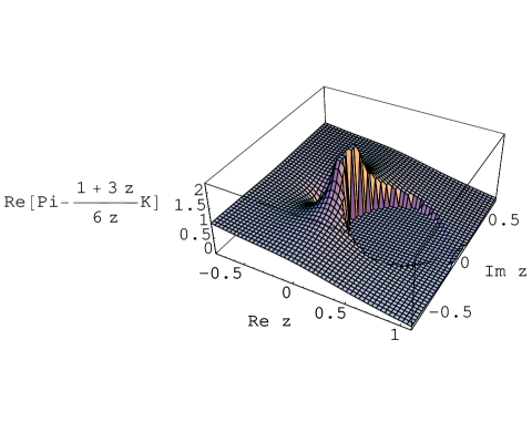
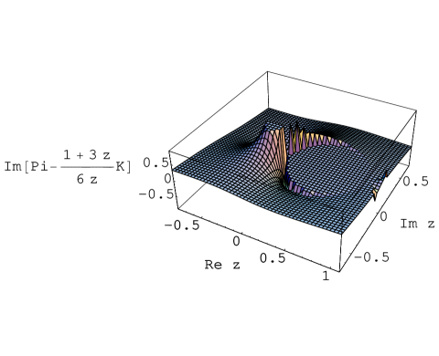
Figure 1: Profile of the left side of Equation (2) as a complex-valued function, with the real variable $x$ promoted to a complex variable $z$.

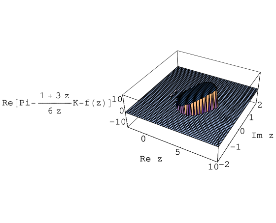
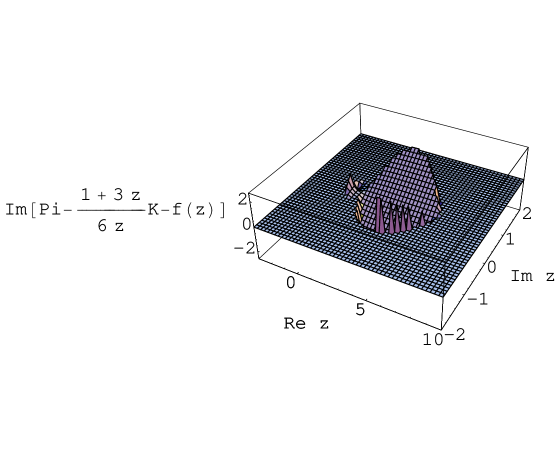
Figure 2: Examination of the validity of second portion of Equation (2) with a complex variable $z$, where $f(z)\equiv-{\pi\over 12}{(z-1)^{3/2}\sqrt{1+3z}\over z}$.

References

- [1] P. F. Byrd and M. D. Friedman, Handbook of Elliptic Integrals for Engineers and Scientists, Springer Verlag, Berlin (1971).
- [2] M. Abramowitz and I. A. Stegun, Handbook of Mathematical Functions, Dover Publications, New York (1972).
- [3] I. S. Gradshteyn and I. M. Ryzhik, Table of Integrals, Series, and Products, Academic Press, San Diego (2000).
- [4] Wolfram Research, Inc., Mathematica Edition: Version 5.0, Wolfram Research, Inc., Champaign, IL (2003).
- [5] B. Almgren, Arkiv för Physik 38, 161 (1968).
- [6] S. Bauberger, F. A. Berends, M. Bohm and M. Buza, Nucl. Phys. B 434, 383 (1995) [arXiv:hep-ph/9409388].
- [7] A. I. Davydychev and R. Delbourgo, J. Phys. A 37, 4871 (2004) [arXiv:hep-th/0311075].
- [8] W. E. Boyce and R. C. DiPrima, Elementary Differential Equations and Boundary Value Problems (2nd Edition), John Wiley & Sons , New York (1969).