Sources of contamination to weak lensing three-point statistics: constraints from N-body simulations

Abstract

We investigate the impact of the observed correlation between a galaxies shape and its surrounding density field on the measurement of third order weak lensing shear statistics. Using numerical simulations, we estimate the systematic error contribution to a measurement of the third order moment of the aperture mass statistic (GGG) from three-point intrinsic ellipticity correlations (III), and the three-point coupling between the weak lensing shear experienced by distant galaxies and the shape of foreground galaxies (GGI and GII). We find that third order weak lensing statistics are typically more strongly contaminated by these physical systematics compared to second order shear measurements, contaminating the measured three-point signal for moderately deep surveys with a median redshift $z_{\rm m}\sim 0.7$ by $\sim 15\%$. It has been shown that accurate photometric redshifts will be crucial to correct for this effect, once a model and the redshift dependence of the effect can be accurately constrained. To this end we provide redshift-dependent fitting functions to our results and propose a new tool for the observational study of intrinsic galaxy alignments. For a shallow survey with $z_{\rm m}\sim 0.4$ we find III to be an order of magnitude larger than the expected cosmological GGG shear signal. Compared to the two-point intrinsic ellipticity correlation which is similar in amplitude to the two-point shear signal at these survey depths, third order statistics therefore offer a promising new way to constrain models of intrinsic galaxy alignments. Early shallow data from the next generation of very wide weak lensing surveys will be optimal for this type of study.

1 Introduction

Weak gravitational lensing represents a powerful tool to investigate the large-scale distribution of matter. The majority of lensing results to date have focused on using two-point shear statistics to constrain the matter density parameter $\Omega_{\rm m}$ and the matter power spectrum normalisation $\sigma_{8}$ [van Waerbeke et al. 2001, Hoekstra et al. 2002, Bacon et al. 2003, Jarvis et al. 2003, Hamana et al. 2003, Rhodes et al. 2004, Heymans et al. 2005, van Waerbeke et al. 2005, Massey et al. 2005, Semboloni et al. 2006, Hoekstra et al. 2006, Massey et al. 2007, Benjamin et al. 2007, Fu et al. 2008]. As these two parameters are strongly degenerate however there is great interest in measuring higher order statistics as their combination with the two-point shear statistics can effectively break the degeneracy between $\Omega_{\rm m}$ and $\sigma_{8}$ [Bernardeau et al. 1999]. To date, there have been few measurements of three-point shear statistics [Bernardeau et al. 2002, Jarvis et al. 2004, Pen et al. 2003]. These results found that the three-point shear statistics were significantly affected by systematics even when the two-point statistics showed a very low systematic level. The aim of this paper is to investigate, by using $\Lambda$CDM N-body simulations, whether the intrinsic alignment of the sources (see for example Heavens et al. 2000) and the correlation between the shear field and the intrinsic ellipticity of the sources [Hirata & Seljak 2004, Heymans et al. 2006, Mandelbaum et al. 2006, Hirata et al. 2007] can explain the presence of some systematics.

In the weak lensing regime the observed ellipticity $e_{\rm o}$ of a source galaxy is related to the original ellipticity $e_{\rm s}$ through:

$$e_{{\rm o}}\simeq e_{\rm s}+\gamma,$$ (1)

where $\gamma=\gamma_{1}+{\rm i}\gamma_{2}$ is the complex shear, and $e$ is the complex ellipticity defined as

$$e=\frac{1-\beta^{2}}{1+\beta^{2}}\frac{{\rm exp}{(2{\rm i}\phi)}}{R},$$ (2)

where $\phi$ is the angle between the semi-major axis and the $x$-axis, $\beta$ is the ratio between the semi-major and semi-minor axis and $R$ is the response of a galaxy to weak lensing shear field. Note that in the commonly used KSB method [Kaiser et al. 1995] the responsivity $R$ is expressed by the polarizability tensor which is computed for each object and relates the measured weighted ellipticity to the shear field. In this analysis where no weight is applied we are able to calculate the average responsivity for our sample finding $R=0.89$ (see Rhodes et al. 2000, Bernstein & Jarvis 2002).

The two- and three-point ellipticity correlation functions between the observed galaxies $a$, $b$ and $c$ are given by :

$$\langle e_{{\rm o}}^{a}e_{{\rm o}}^{b}\rangle=\langle e_{\rm s}^{a}e_{\rm s}^{b}\rangle+{\rm GI}+\langle\gamma^{a}\gamma^{b}\rangle,$$ (3)

$$\langle e_{{\rm o}}^{a}e_{{\rm o}}^{b}e_{{\rm o}}^{c}\rangle=\langle e_{\rm s}^{a}e_{\rm s}^{b}e_{\rm s}^{c}\rangle+{\rm GGI}+{\rm GII}+\langle\gamma^{a}\gamma^{b}\gamma^{c}\rangle,$$ (4)

where the GI, GII and GGI terms are:

$${\rm GI}=\langle e_{\rm s}^{a}\gamma^{b}\rangle+\langle e_{\rm s}^{b}\gamma^{a}\rangle,$$ (5)

$${\rm GII}=\langle\gamma^{a}e_{\rm s}^{b}e_{\rm s}^{c}\rangle+\langle\gamma^{b}e_{\rm s}^{c}e_{\rm s}^{a}\rangle+\langle\gamma^{c}e_{\rm s}^{a}e_{\rm s}^{b}\rangle,$$ (6)

$${\rm GGI}=\langle\gamma^{a}\gamma^{b}e_{\rm s}^{c}\rangle+\langle\gamma^{b}\gamma^{c}e_{\rm s}^{a}\rangle+\langle\gamma^{c}\gamma^{a}e_{\rm s}^{b}\rangle.$$ (7)

One assumes that galaxies are intrinsically randomly oriented so the measurement of the observed ellipticity is an unbiased estimator of the shear. In a similar way one assumes that the measurement of the correlation between ellipticity of pairs and triplets of galaxies is an unbiased estimator of the second and third order moments of the weak lensing shear field. However, this assumption is not correct for galaxies that are physically close as an intrinsic alignment between the galaxies can be induced by a tidal field which acts on cluster scales as has been observed by Brown et al. (2002) and Mandelbaum et al. (2006). These results imply that the first term of Equation (3), hereafter referred as to II, and the first term of Equation (4), hereafter referred as to III, are non-zero and they systematically affect the value of the two- and three-point weak lensing shear statistics estimated through the observed ellipticity alignment. It has been shown (King & Schneider 2002, 2003, Heymans & Heavens 2003, King 2005) that this bias can be removed if close pairs of galaxies are downweighted in the lensing analysis, something which is possible only when the redshift for each individual galaxy can be reliably estimated. For moderately deep surveys such as CFHTLS Wide (Fu et al. 2008), the intrinsic alignment does not significantly affect the estimation of the normalisation of power spectrum $\sigma_{8}$. However, once the redshift information is added it is possible to exploit all the information carried by the shear signal, by using three-dimensional measurements. The measurement of the two-point shear statistics in redshift bins, i.e. tomography (Semboloni et al. 2006) and the 3D-lensing (Heavens et al. 2006, Kitching et al. 2007), are particularly promising to constrain the equation of state of dark energy, but are also more susceptible to stronger contamination by intrinsic alignment (Heymans et al. 2004, King 2005).

A more subtle effect is the correlation between the induced weak lensing shear and the foreground intrinsic ellipticity field, also called “shear-shape” correlation [Hirata & Seljak 2004]. This effect can be explained as follows. Consider a background galaxy with redshift $z^{a}$ whose light is deflected by a foreground over-density at $z^{b}$. Consider now a galaxy at redshift $z^{b}$ stretched by the tidal forces generated by the dark matter over-density. Then the term $\langle\gamma^{a}e_{\rm s}^{b}\rangle\neq 0$. Similarly, for the three-point shear statistics, one can consider two sources with redshift $z^{a}$ and $z^{b}$ whose light is deflected by the same halo hosting a galaxy at redshift $z^{c}<z^{a},z^{b}$: in this case the term $\langle\gamma^{a}\gamma^{b}e_{\rm s}^{c}\rangle\neq 0$. Finally, one can imagine a background galaxy with redshift $z^{a}$ being sheared by an over-density hosting galaxies at redshifts $z^{b}$ and $z^{c}$ with the result $\langle\gamma^{a}e_{s}^{b}e_{s}^{c}\rangle\neq 0$.

The first measurement of the shear-shape systematic effect on the Sloan Digital Sky Survey (SDSS) data by Mandelbaum et al. (2006) has been refined by Hirata et al. (2007), which uses subsamples from the SDSS and 2SLAQ surveys to check the dependence of the shear-shape correlation on the color, morphology and luminosity of galaxies. Hirata et al. (2007) predict that the shear-intrinsic alignment coupling could cause an underestimate of the normalisation of the power spectrum $\sigma_{8}$ of up to ten percent. Heymans et al. 2006 (hereafter H06) provide a simple toy model to investigate this effect using N-body simulations which we describe in more detail in section 3. This simple model also predicts a shear-intrinsic alignment of $10\%$ of the expected weak lensing shear signal, and provides a good fit to the measurements of Hirata et al. (2007). In contrast to the intrinsic alignment systematic that affects the lensing measured in the same tomographic redshift slice, the shear-shape systematic affects galaxies in very different tomographic redshift bins. The shear-shape systematic strongly reduces the precision with which one is able to constrain the dark energy equation of state by tomography, as shown by Bridle & King (2007).

Adopting the same strategy as H06, we analyse a set of $\Lambda$CDM N-body simulations, in order to compare the amplitude of the intrinsic ellipticity and the shear-shape terms to the three-point weak lensing shear statistics.

The paper is organised as follows. In the section 2 we define the quantities and we describe the method used in this work to measure three-point statistics. In section 3 we describe the simulations used in this work. In section 4 we present measurements of the three-point intrinsic alignment, and in section 5 we show the evolution of the three-point coupling between shear and intrinsic ellipticity fields as a function of the redshift distribution of the lenses and sources. We also provide a fitting formula for the three-point shear-ellipticity correlation from different galaxy models. We conclude in section 6.

2 Three point shear statistic measurement

Following the approach of Pen et al. (2003) and Jarvis et al. (2004) we define the complex ‘natural components’ of the three-point shear correlation functions (Schneider & Lombardi 2003) for a triangle of vertex ${\bf X}_{1}$, ${\bf X}_{2}$ and ${\bf X}_{3}$ and separations vectors ${\bf r}_{1}={\bf X}_{3}-{\bf X}_{2}$ ${\bf r}_{2}={\bf X}_{1}-{\bf X}_{3}$, ${\bf r}_{3}={\bf X}_{2}-{\bf X}_{1}$:

$$\Gamma_{0}(r_{1},r_{2},r_{3})=\langle\gamma({\bf r}_{1})\gamma({\bf r}_{2})\gamma({\bf r}_{3}){\rm e}^{[-2{\rm i}(\phi_{1}+\phi_{2}+\phi_{3})]}\rangle,$$ (8)

$$\Gamma_{1}(r_{1},r_{2},r_{3})=\langle\gamma^{\star}({\bf r}_{1})\gamma({\bf r}_{2})\gamma({\bf r}_{3}){\rm e}^{[-2{\rm i}(-\phi_{1}+\phi_{2}+\phi_{3})]}\rangle,$$ (9)

$$\Gamma_{2}(r_{1},r_{2},r_{3})=\langle\gamma({\bf r}_{1})\gamma^{\star}({\bf r}_{2})\gamma({\bf r}_{3}){\rm e}^{[-2{\rm i}(\phi_{1}-\phi_{2}+\phi_{3})]}\rangle,$$ (10)

$$\Gamma_{3}(r_{1},r_{2},r_{3})=\langle\gamma({\bf r}_{1})\gamma({\bf r}_{2})\gamma^{\star}({\bf r}_{3}){\rm e}^{[-2{\rm i}(\phi_{1}+\phi_{2}-\phi_{3})]}\rangle,$$ (11)

where $\gamma$ is the complex shear and we indicate with $\gamma^{\star}$ the complex conjugate of $\gamma$. The choice of the directions $\phi_{i}$ along which one projects the shear are free as long as the value of $\Gamma_{i}$ does not depend on the triangles orientation. Assuming that the Universe is homogeneous and isotropic, the eight real components of the shear correlation function depend on the side-lengths of the triangle, $r_{1}$, $r_{2}$, and $r_{3}$. Thus we prefer to use a derived statistic which is easier to visualize and interpret, namely the third order moment of the aperture mass statistic.

The complex aperture mass is defined as :

$$M_{\vartheta}=M_{\rm ap}+{\rm i}M_{\times}=\int d^{2}\bm{r}Q_{\vartheta}(r)\gamma(\bm{r})e^{(-2{\rm i}\phi)},$$ (12)

where $Q_{\vartheta}(r)$ is a filter of characteristic size $\vartheta$. Using the aperture mass statistics allows one to uniquely separate the E-mode ($M_{\rm ap}$) and B-mode ($M_{\times}$) component of the measured shear (Crittenden et al. 2002), providing a powerful test for systematics. Indeed, weak lensing shear fields are E-type fields; thus the presence of other sources of distortion can be revealed by measuring $M_{\times}$ statistics which are non-zero only for B-mode fields.

In practice, the variance and the third order moment of the aperture mass can be measured as a function of the two- and three-point shear statistics, respectively [Crittenden et al. 2002, Pen et al. 2002]. Estimating the third order moment of the aperture mass through three-point correlation functions is preferred however, as it yields a higher signal-to-noise ratio than the direct measurement of the moments of the integral of Equation (12) [Schneider et al. 2002]. In addition, in the case of real data, where masked regions are present, the estimate of the aperture mass statistic through the measurement of the correlation function is unbiased, whilst the direct measurement of the moments is biased. By choosing the following filter,

$$Q_{\vartheta}(r)=\frac{1}{2\pi\vartheta^{2}}\Big{(}1-\frac{r^{2}}{2\vartheta^{2}}\Big{)}\exp\Big{(}-\frac{r^{2}}{2\vartheta^{2}}\Big{)},$$ (13)

the four components of the third order moment
$\langle M_{\rm ap}^{3}\rangle$, $\langle M_{\rm ap}^{2}M_{\times}\rangle$,$\langle M_{\rm ap}M_{\times}^{2}\rangle$ and $\langle M_{\times}^{3}\rangle$ can be obtained through integration of the three-point shear statistics $\Gamma_{i}$ (see for example equations (45), (50) of Jarvis et al. 2004 and equations (61-71) of Schneider et al. 2005). There are other advantages of using aperture mass statistics defined by using Equation (13). This filter has infinite support but the exponential cutoff allows one to assume a finite support for real calculations. Furthermore, the Fourier transformed filter,

$$I(\eta)=\frac{1}{2\pi}\frac{\eta^{4}}{4}{\rm exp}(-\eta^{2})$$ (14)

were we defined $\eta=s\vartheta$, is a very narrow window filter, probing essentially modes with $s\sim 2/\vartheta$.

We measure the four complex $\Gamma_{i}$ components using a binary tree code built following the model suggested by Pen et al. (2003). We assign to each box an ellipticity $(e_{1},e_{2})$ and a position $(x,y)$ which are the average of the ellipticity and positions of the galaxies contained in the box. To each box we assign also a weight which is the sum of the weights assigned to each galaxy. The characteristic size $l_{i}$ of each box is chosen to be the distance between the centre of the box and the furthest galaxy contained in the box. The correlation between triplets is computed for triangle of sizes $l_{1}$, $l_{2}$, $l_{3}$ satisfying the conditions:

$$\frac{l_{1}+l_{2}}{r_{3}}<0.1,~{}~{}\frac{l_{2}+l_{3}}{r_{1}}<0.1,~{}~{}\frac{l_{3}+l_{1}}{r_{2}}<0.1~{}.$$ (15)

Each triangle is ordered such that $r_{3}\leq r_{2}\leq r_{1}$. We measure $\Gamma_{i}$ for triangles with $r_{3}$ between $5~{}\rm{arcsec}$ and $80~{}\rm{arcmin}$, ranging in logarithmic bins of width $\log(r_{3})=0.1$. With this choice, we can assume that the distance between each pair of galaxies within the boxes that we are correlating has a maximum error of one bin. Finally we integrate $\Gamma_{i}$ using equation (45) and equation (50) of Jarvis et al. (2004). As we already anticipated, the filter defined by Equation (13) for a given size $\vartheta$ has infinite support so we ideally would need to measure $\Gamma_{i}$ at all scales to perform the integral giving the components of the the third-order moment of the aperture mass. However the integral is significant only for triangles up to $r_{3}\simeq 4\vartheta$, implying that our measurement of the third order moment is reliable up to an angular scale $\vartheta\simeq 20~{}\rm{arcmin}$. We tested our algorithm against the direct measurement of the third-order moment of the aperture mass on $\Lambda$CDM simulations in fields of $25~{}{\rm deg^{2}}$ and we found indeed a good agreement between the two methods at these scales.

Throughout the paper we use only the aperture mass statistics and we call the systematic produced by the intrinsic alignments on the second and third order moments of the aperture mass II and III, respectively. Similarly, we call GI the second order moment measured by using the filter defined by the Equation (13) produced by the shear-shape coupling and we call the third order moments GGI and GII. Finally, we call the second and third order moments of aperture mass produced by a weak lensing field GG and GGG.

In order to know the importance of the GGI, GII and III when estimating the third order moment of the aperture mass GGG using the observed ellipticity of galaxies we have to compare those terms with the third order moment of the aperture mass produced by a weak lensing shear field. In the quasi-linear perturbation theory, the perturbation of the density field $\delta$ is considered to be small so that it can be developed in a series $\delta=\delta^{(1)}+\delta^{(2)}+....$, where $\delta^{(1)}$ is the linear evolving density field and $\delta^{(n)}\propto{\mathcal{O}}((\delta^{(1)})^{n})$. In this approximation the $\langle M_{\rm ap}^{3}\rangle_{\vartheta}$ weak lensing signal is (Fry 1984, Schneider et al. 1998) :

$${\rm GGG}\equiv\langle M_{\rm ap}^{3}\rangle_{\vartheta}=\frac{1}{2\pi}\frac{81H_{0}^{6}}{4c^{6}}\Omega_{\rm m}^{3}\int^{w_{H}}_{0}dw\frac{g^{3}(w)}{a^{3}(w)f_{\kappa}(w)}$$ (16)

$$\times\int_{0}^{\infty}d^{2}{\bf s}_{1}P\Big{(}\frac{s_{1}}{f_{\kappa}(w)},w\Big{)}I(s_{1}\vartheta)$$

$$\times\int_{0}^{\infty}d^{2}{\bf s}_{2}P\Big{(}\frac{s_{2}}{f_{\kappa}(w)},w\Big{)}I(s_{2}\vartheta)$$

$$\times I(|{\bf s}_{1}+{\bf s}_{2}|\vartheta)F_{2}({\bf s}_{1},{\bf s}_{2}),$$

with

$$g(w)=\int_{w}^{w_{H}}dw^{\prime}p_{s}(w^{\prime})\frac{f_{\kappa}(w-w^{\prime})}{f_{\kappa}(w^{\prime})}.$$ (17)

$f_{\kappa}(w)$ is the comoving angular diameter distance, $P(s,w)$ is the 3 dimensional power spectrum of matter fluctuations, $p_{s}(w)$ is the comoving distance distribution of the sources, $I(s\vartheta)$ is the Fourier transform of the filter as defined by Equation (14) and $F_{2}({\bf s}_{1},{\bf s}_{2})$ is the coupling between two different modes of density fluctuations characterised by the wave vectors ${\bf s}_{1}$ and ${\bf s}_{2}$. We compute $F_{2}({\bf s}_{1},{\bf s}_{2})$ using the fitting formula suggested by Scoccimarro & Couchman (2001).

3 N-Body simulations and galaxy models

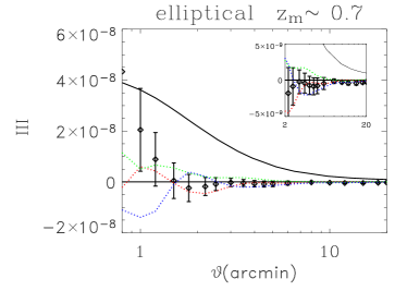
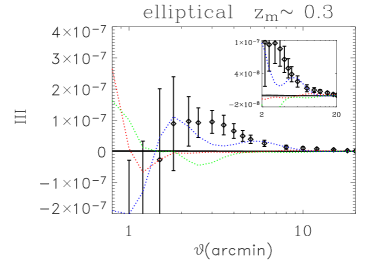
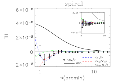
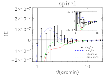
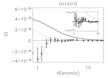
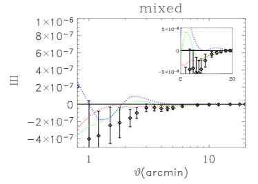
Figure 1: Left panel: $\langle M_{\rm ap}^{3}\rangle$ signal generated by the intrinsic alignments (III) as a function of the angular size $\vartheta$. By comparing the E-modes (black diamond) with the expected shear signal (black solid line) one can determine the level of contamination produced by the existence of intrinsic alignments between galaxies. The shear signal has been computed using Equation (16) for the same redshift distribution used to compute the intrinsic alignment term III. The median redshift of this distribution is $z_{\rm m}\sim 0.7$. The error-bars are the dispersion of the average signal measured in twelve independent realizations. The B-mode signal, $\langle M_{\times}^{3}\rangle$, and the E/B components, $\langle M_{\rm ap}^{2}M_{\times}\rangle$ and $\langle M_{\rm ap}M_{\times}^{2}\rangle$, are shown dashed and for clarity we chose not to plot the error bars. The right panel shows the same results as the left panel for a lower redshift sample of galaxies $0<z<0.4$. For this redshift distribution characterised by $z_{\rm m}\simeq 0.3$, the predicted shear signal GGG $\sim 10^{-9}$ is indistinguishable from zero in this plot.

In this analysis we use the same set of simulations used as in H06. We recall here only the main characteristics and refer the reader to H06 for more detailed information. The N-body simulation is a box of $300h^{-1}{\rm Mpc}$ realized using a $\Lambda$CDM cosmology. The matter density parameter is $\Omega_{\rm m}=0.3$, the cosmological constant is $\Omega_{\Lambda}=0.7$, the normalisation of the power spectrum of matter fluctuations is $\sigma_{8}=0.8$, the reduced Hubble constant is $h=0.7$ and the baryon density parameter is $\Omega_{\rm b}h^{2}=0.2$. The simulation started at redshift $z=60$ and evolved to $z=0$. Twelve lines of sight were built by stacking boxes back along the $z$-axis with random shifts between the boxes in the $x$ and $y$ direction in order to avoid artificial correlations, producing (almost) independent realisations.

The over-densities are identified using a ‘friends of friends’ group finder, which allows one to identify the halos. The particle mass of $1.7\times 10^{10}~{}h^{-1}\rm{M_{\odot}}$ allows us to find bound halos with masses larger than few $10^{11}~{}h^{-1}\rm{M_{\odot}}$. The halos are then populated with galaxies. The luminosity is assigned following the conditional luminosity function (CLF) of Cooray & Milosavljevic (2005) and the ellipticity is assigned using a toy model that has been shown effective at reproducing the observations of Mandelbaum et al. (2006) and Hirata et al. (2007). In this model, elliptical galaxies are given the same ellipticity as their parent halos. Spiral galaxies are modeled as a thick disk oriented almost perpendicular to the angular momentum vector of the halo with a mean random misalignment of $\sim 20~{}\rm{deg}$ (van den Bosch et al. 2002, Heymans et al. 2004). At each identified dark matter halo in the simulations we generate both a spiral and an elliptical galaxy so that we can investigate the results as a function of morphology. We define the ellipticity of the model galaxies using Equation (2). The resulting ellipticity distribution has a zero mean and dispersion of $\sigma_{e}=0.33$.

In the results that follow we present three models: one composed exclusively of spiral galaxies, one composed exclusively of elliptical galaxies and one containing both the morphologies denoted ‘mixed’. The mixed model has been built following Cooray & Milosavljevic (2005) and it contains $\sim 30\%$ elliptical galaxies. The mixed model is the most realistic model out of the three tested; the GI and II components predicted using the mixed model agree with the ones measured using the SDSS data (Mandelbaum et al. 2006, Heymans et al. 2006, Hirata et al. 2007). The number density of the final catalogue, which contains galaxies between $0<z<1$ and is complete up to $r=25.5$, is about 5 per $\rm{arcmin^{2}}$, which is considerably lower than what is expected for such a survey. This is due on one hand to the fact that the low resolution of the simulations implies the loss of low-mass halos (only halos with mass larger than few $10^{11}~{}\rm{M_{\odot}}$ are identified) and that each halo is populated with only one galaxy. The lack of the low-mass halos and satellite galaxies is the main limitation of our model and this point is discussed further in the conclusions.

Finally, these same N-body simulation which have been populated with galaxies are ray-traced to produce twelve projected mass distributions $\kappa$ for a source plane at $z_{\rm s}=0.45$ and for $z_{\rm s}=1.05$. We use these simulated $\kappa$ maps in section 5 to study the shear-shape effect. Each projected mass map covers an area of $5\times 5~{}\rm{deg^{2}}$ in $2048\times 2048$ pixels.

4 Intrinsic ellipticity alignment

In this section we report the third order moment components of the aperture mass given by the intrinsic alignment of the sources. We measure the third order moment of the aperture mass for a survey with maximum depth $z\sim 1$ and compare the measured intrinsic alignment to the expected weak lensing GGG signal from Equation (16). The redshift distribution of the sources $p_{\rm s}(w)$ is computed directly from the catalogues used for the III measurement so that both III and GGG terms have been computed for the same survey.

Figure 1 shows the three-point intrinsic alignment for our three toy models: elliptical (upper panel), spiral (middle panel) and mixed (lower panel) for two survey types; one with a median redshift of $z_{\rm m}\sim 0.7$ (left panels) and the other with $z_{\rm m}\sim 0.3$ (right panels). The error-bars on the measurements have been computed as the dispersion in the average signal measured in the twelve realisations, thus they include statistical and cosmic variance. For the moderately deep survey ($z_{\rm m}\sim 0.7$) the III term is consistent with zero for all the three models. This result is in agreement with H06 who find that the two-point intrinsic ellipticity term II, is consistent with zero for the same survey characteristics. As expected, however, we find that when the redshift depth of the survey decreases the III term becomes significant due to the fact that for lower redshift galaxies, a given angular distance corresponds to a physically closer triplet. Comparing now the results for the three different toy models for this shallow survey we find very different results. Figure 1 shows that the III term is significantly positive for $\vartheta>2$ arcmin for elliptical galaxies (upper right panel) meanwhile it is slightly negative for the spiral model (middle right panel) and significantly negative for the mixed model (lower right panel). The mixed model contains roughly $70\%$ of spiral galaxies and $30\%$ of elliptical galaxies, such that the most frequent triangle in the three-point measurement contains two spiral galaxies and one elliptical galaxy. As this type of correlation does not exist when one considers only elliptical or only spiral morphologies, the mixed result is not a weighted average of the result containing only elliptical or spiral galaxies. We verified that the third order moment of the aperture mass is indeed negative when we correlate triplets containing two spirals and one elliptical. Figure 1 shows that for shallow surveys ($z_{\rm m}\lower 2.15277pt\hbox{$\;\buildrel<\over{\sim}\;$}0.5$) the intrinsic alignment dominates the signal and suggests that also for deeper surveys the intrinsic alignment could affect the measured the three-point weak lensing signal.

In order to quantify the effect of the intrinsic alignment on the weak lensing shear statistics we compare the amplitude of the two- and three-point intrinsic alignment signal II and III with the expected weak lensing signal, respectively GG and GGG, for different shallow surveys. Figure 2 shows the amplitude of the II/GG (left panel) and III/GGG (right panel) ratios for three different surveys depth using the mixed model as an example. We find that for a given survey depth, the ratio between the III term and expected weak lensing third order moment GGG, is generally higher than the ratio between the II term and the variance of the weak lensing aperture mass GG. One can think to reduce significatively the intrinsic ellipticity contamination to the two- and three-point shear statistics by removing very low redshift sources ($z\lower 2.15277pt\hbox{$\;\buildrel<\over{\sim}\;$}0.2$ ) which contribute to the intrinsic alignment signal but not to the weak lensing signal. We checked that the ratio II/GG and III/GGG drops on small scales $\vartheta\lower 2.15277pt\hbox{$\;\buildrel<\over{\sim}\;$}10$ arcmin if galaxies with $z<0.2$ are rejected, but it is almost unchanged at larger scales.

Figure 1 and Figure 2 show that without a technique to correct for the intrinsic alignment it will be impossible have a precise measurement of the three-point shear statistics in shallow surveys ($z_{\rm m}\lower 2.15277pt\hbox{$\;\buildrel<\over{\sim}\;$}0.5$). For moderately deep surveys like the CFHTLS Wide, the ratio III/GGG is consistent with zero as shown by the left panels of Figure 1. However, for larger surveys, where the statistical and cosmic variance are small the intrinsic alignment could still play a role in the precision with which one can constrain the cosmological parameters. This can be seen in Figure 2 where for a relatively deep survey ($z<0.8$) the intrinsic alignment contribution is likely to be non-zero, specially for the third order moment of the aperture mass.

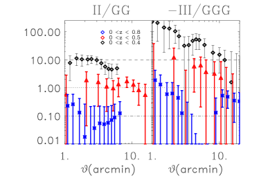
Figure 2: Left side: ratio between the intrinsic alignment (II) and the aperture mass variance (GG) for three surveys. Right side: ratio between III the expected weak lensing signal (GGG) for the same surveys as the left panel. The galaxy model is a mixed model. The expected second and third order aperture mass moment are computed for each survey by using the same source redshift distribution used to measure the III and II terms. These distributions are characterized by: $z_{\rm m}\sim 0.31$ for source distribution between $0<z<0.4$, $z_{\rm m}\sim 0.4$ for source distribution $0<z<0.5$ and source distribution $z_{\rm m}\sim 0.6$ for $0<z<0.8$.

This result strongly supports the need for reliable photometric redshift for weak lensing studies. Moreover, Figure 2 demonstrates that if the redshift is known, one can select sources in order to enhance the II and III signal relative to the contribution of the GG and GGG terms to the measured two and three-point shear statistics. This is an important result since one needs a good intrinsic alignment model to be able to remove this contribution from the two-point (three-point) weak lensing shear statistics (King 2005). The fact that the III/GGG signal is more significant than the II/GG signal implies that it may be easier to study intrinsic alignments using three-point statistics. In this respect Figure 2 shows that large multi-band surveys like SDSS and KIDS or PanSTARRS, represent excellent surveys to investigate and model the intrinsic alignment of elliptical and spiral galaxies.

5 Shear ellipticity alignment

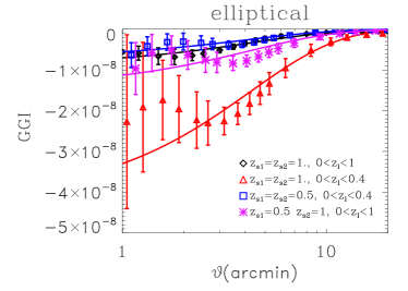
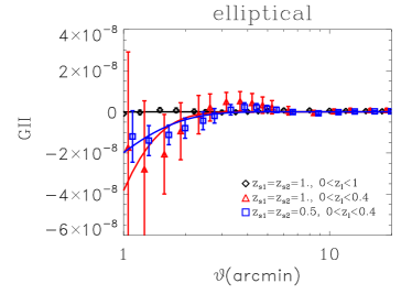
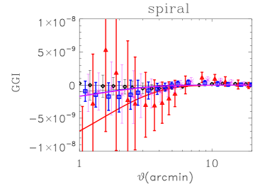
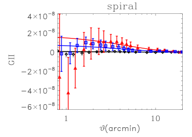
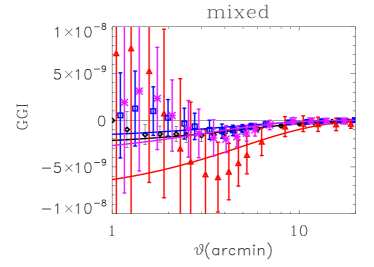
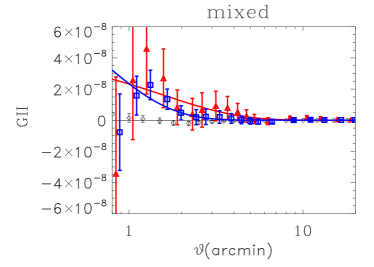
Figure 3: GGI (left panels) and GII (right panels) components for different redshift slices and three galaxy models: elliptical (upper panels), spiral (middle panels) and mixed (lower panel). We show three sets of measurements corresponding to: a lens distribution $0<z_{\rm l}<1$ and a source distribution $z_{\rm s}=1.05$ (black diamonds), $0<z_{\rm l}<0.4$ and $z_{\rm s}=1.05$ (red triangles) and $0<z_{\rm l}<0.4$ and $z_{\rm s}=0.45$ (blue squares). For the GGI component we also include a third model which contains lenses $0<z_{\rm l}<0.4$ and sources in two different planes: one at $z_{\rm s}=0.45$ and the other at $z_{\rm s}=1.05$. Error bars represent the dispersion in the average value between the twelve simulations. For each measurement of the GGI and GII components we show the best-fit model (solid lines) obtained by rescaling the redshift distribution dependence given by equations (19) and (21) with the angular dependence described by Equation (22).

In this section we study the behavior of the three-point shear-shape coupling which, as it has been detailed in equations (6) and (7), can be divided in two terms, namely GGI and GII. One would expect these two terms to have a different behavior as a function of the redshift distribution of the lenses and of the sources. The GII term depends on the intrinsic ellipticity correlation between two pairs of galaxies thus it should be significant only for triplets which contain foreground galaxies closer than the scales on which tidal forces act. The GGI term correlates the shape of lensed background galaxies with the intrinsic shape of a foreground galaxy so it is expected to be significant also when correlating well-separated redshift slices, similarly to what has been found for the GI term (Bridle & King 2007). Using both ray tracing simulations with redshift $z_{\rm s}=0.45$ and $z_{\rm s}=1.05$ and dividing the foreground galaxies into redshift bins, we study the evolution of the GII and GGI terms as a function of the source and lens redshift distribution. Figure 3 shows the amplitude of the GGI (left panels) and GII (right panels) terms for elliptical (upper panels), spiral (middle panels) and the mixed model (lower panels) for different redshift bins. We note that the amplitude of the GGI and GII terms for a given survey depends on the morphology of the galaxies. The elliptical galaxies show a significant negative GGI signal whereas the spiral model shows a GGI signal which is consistent with zero. Finally, the mixed model shows a slightly negative GGI signal.

The GII component for the spiral galaxies show an angular dependence similar to the one of the elliptical galaxies and interestingly the signal at intermediates scales ($2\lower 2.15277pt\hbox{$\;\buildrel<\over{\sim}\;$}\vartheta\lower 2.15277pt\hbox{$\;\buildrel<\over{\sim}\;$}10$ arcmin) is stronger than for the elliptical galaxy model. Similarly to what we previously found for the III term, the mixed model GII term is different from the one obtained using only elliptical or spiral galaxies. This is likely to be a consequence of the fact that for the two morphologies the ellipticity depends differently on the properties of the parent halos, which also could explain the difference in results for the III term. To understand this phenomena would require building a model for the three-point correlation function between weak lensing shear and tidal field, in a similar analysis as that of the two-point correlation function presented in Hirata & Seljak (2004). This however is beyond the scope of this paper.

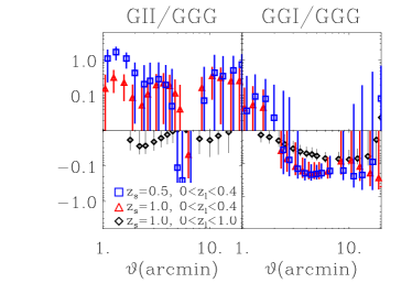
Figure 4: Left side: ratio between the GII term and the expected signal (GGG) for three shallow surveys. Right side: ratio between the GGI term and the GGG signal for the same surveys as the left panel. The galaxy model is a mixed model. We used the same surveys as Figure 3. The GGG signal has been computed by taking $z_{s}=1.05$ (black diamonds and red triangles) and $z_{s}=0.45$ (blue squares).

In order to allow a more quantitative comparison between the weak lensing three-point shear signal and the systematics GII and GGI, we report in Figure 4 the ratio between the terms GII and GGG (left panel) and GGI and GGG (right panel) for the mixed model.

Table 1: Summary table of the best fit parameters of the GGI (first four columns) and GII (last three columns) terms for elliptical (upper lines), spiral (middle lines) and mixed (lower lines) galaxies using Equation (19) and Equation (21). The values the parameters $\vartheta_{0}$ are given in arcmin, the values of the parameter $A$ are given in units of $10^{-7}h~{}{\rm Mpc}^{-1}$. For each model we report the value of the reduced $\chi^{2}$.

			GGI				GII
		$z_{\rm s}=1$	$z_{\rm s}=1$	$z_{\rm s}=0.5$	$z_{{\rm s}}=1;0.5$	$z_{\rm s}=1$	$z_{\rm s}=1$	$z_{\rm s}=0.5$
		$z_{\rm l}<1$	$z_{\rm l}<0.4$	$z_{\rm l}<0.4$	$z_{\rm l}<0.4$	$z_{\rm l}<1$	$z_{\rm l}<0.4$	$z_{\rm l}<0.4$
	$\vartheta_{0}$	$4.39\pm 0.38$	$4.23\pm 0.33$	$4.06\pm 0.45$	$4.25\pm 0.42$	$0.37\pm 2.02$	$0.38\pm 0.34$	$0.60\pm 0.23$
elliptical	$A$	$-0.88\pm 0.09$	$-1.02\pm 0.11$	$-0.47\pm 0.07$	$-0.62\pm 0.08$	$-0.04\pm 0.30$	$-2.56\pm 6.77$	$-1.14\pm 1.34$
	$\chi^{2}$	$1.11$	$0.59$	$0.31$	$0.52$	$4.34$	$0.62$	$0.73$
	$\vartheta_{0}$	$5.12\pm 0.92$	$4.84\pm 1.75$	$3.24\pm 1.73$	$0.38\pm 1.73$	$0.38\pm 0.66$	$1.58\pm 0.70$	$0.62\pm 0.28$
spiral	$A$	$-0.26\pm 0.05$	$-0.19\pm 0.09$	$-0.27\pm 0.07$	$-0.16\pm 0.12$	$0.03\pm 0.11$	$0.22\pm 0.19$	$1.28\pm 1.37$
	$\chi^{2}$	$0.14$	$0.36$	$0.23$	$0.24$	$0.74$	$0.48$	$0.30$
	$\vartheta_{0}$	$2.36\pm 1.40$	$1.46\pm 1.24$	$1.27\pm 0.83$	$1.36\pm 1.52$	$1.94\pm 1.88$	$4.83\pm 0.90$	$4.46\pm 0.92$
mixed	$A$	$-0.15\pm 0.11$	$-0.33\pm 0.38$	$-0.24\pm 0.21$	$-0.15\pm 0.22$	$0.05\pm 0.07$	$0.09\pm 0.02$	$0.09\pm 0.03$
	$\chi^{2}$	$0.55$	$0.51$	$0.30$	$0.49$	$0.29$	$0.55$	$0.40$

To aid future comparisons we provide fits to our results. We make the assumption that for a given triplet the GGI and GII terms can be factorized in two functions: one depending on the comoving distances of lenses and sources modeled as in King (2005) and the other depending on the angular scale. We rewrite the GGI term as:

$${\rm GGI}(w_{\rm s_{1}},w_{\rm s_{2}},w_{\rm L},\vartheta)={\rm E_{GGI}}(w_{\rm s_{1}},w_{\rm s_{2}},w_{\rm L})F(\vartheta),$$ (18)

with:

$${\rm E_{GGI}}(w_{{\rm s}_{1}},w_{{\rm s}_{2}},w_{\rm L})=\int_{0}^{w_{\rm L}}dw_{\rm l}\frac{f_{k}(w_{{\rm s}_{1}}-w_{\rm l})}{f_{k}(w_{{\rm s}_{1}})}$$ (19)

$$\times\frac{f_{k}(w_{{\rm s}_{2}}-w_{\rm l})}{f_{k}(w_{{\rm s}_{2}})}p_{\rm l}(w_{\rm l}),$$

where $w_{\rm L}$ is the maximal comoving distance of the lenses with the condition $w_{\rm L}<{\rm min}(w_{{\rm s}_{1}},w_{{\rm s}_{2}})$, $f_{k}(w)$ is the angular diameter distance, $p_{\rm l}(w_{\rm l})$ is the radial lens distribution and $F(\vartheta)$ is a generic function of the angular scale.

Similarly we factorize GII with the assumption that the intrinsic alignment acts only for pairs of galaxies with the same redshift. Thus we write:

$${\rm GII}(w_{\rm s},w_{L},\vartheta)={\rm E_{GII}}(w_{\rm s},w_{\rm L})F(\vartheta),$$ (20)

with:

$${\rm E_{GII}}(w_{\rm s},w_{\rm L})=\int_{0}^{w_{\rm L}}dw_{\rm l}\frac{f_{k}(w_{{\rm s}}-w_{\rm l})}{f_{k}(w_{{\rm s}})}p_{\rm l}(w_{\rm l})^{2},$$ (21)

with the condition $w_{\rm L}<w_{{\rm s}}$. For a broad source distribution one should integrate Equation (19) and Equation (21) over the source distribution to obtain the average effect. However in our case the ray-tracing, source planes follow a Dirac distribution centered at $z_{\rm s}=0.45$ or $z_{\rm s}=1.05$. The lens distribution $p_{\rm l}(w_{\rm l})$ is measured directly from the galaxy catalogues. We find that these scaling factors provide a good description of the redshift dependence both for the GII and GGI term. With this redshift dependence model we try to model the behavior of the GII and GGI terms as a function of the angular scale. We use a two parameter function $F(\vartheta)$:

$$F(\vartheta)=A~{}\exp(-\vartheta/\vartheta_{0})$$ (22)

where $A$ and $\vartheta_{0}$ are free parameters.

In order to avoid bias from the limiting resolution of the simulations we chose to perform the fit using only angular scales $\vartheta>1$ arcmin. In Figure 3 we compare the measurements of the GGI and GII terms with the best-fit model (solid lines) obtained by using the redshift rescaling defined by the equations (19) and (21) and an angular scale dependence defined by Equation (22) for the elliptical, spiral and mixed galaxies. Figure 5 shows the best fit parameters $A$ and $\vartheta_{0}$ for the GGI (left panel) and the GII (right panel) terms for several redshift slices, for elliptical, spiral and mixed model. These values are also summarized in the table 1 which includes also the reduced $\chi^{2}$ of the fit for both the GGI and GII terms. The small values of the $\chi^{2}$ show that the model we suggest is a good fit to the measured GGI component. However, for the elliptical model the dispersion of the best-fit $A$ parameter between the four redshift slices (see left panel of Figure 5) is larger than the error bars. This suggests that the redshift-dependent rescaling described by the Equation (19) could require some modification. The GII component is generally more noisy than the GGI component, and for this reason it is hard to establish whether the model defined by equations (21) and (22) is a good one. However, for the mixed model, which is our most realistic model, the GII term can be fairly well described by our fitting function. Increasing the size of simulations in future analyses will allow us to improve upon these models.

Because of the different dependence on the morphology of galaxies and on the redshift distribution of the sources and lenses for the III, GGI and GII terms, one may be interested in knowing the total effect of the intrinsic alignments and of the shear-coupling on the three-point shear for realistic surveys. Figure 6, shows the ratio between the sum of GGI, GII and III terms and the expected weak lensing signal for several redshift distributions for both the elliptical (left panel) and mixed (right panel) model.

For shallow surveys ($z_{\rm l}\lower 2.15277pt\hbox{$\;\buildrel<\over{\sim}\;$}0.5$), the ratio is largely dominated by the III term. This is true both for elliptical and mixed model with the difference that for the elliptical galaxies the intrinsic alignment enhances the weak lensing shear signal whereas for the mixed model it suppresses the weak lensing signal. For a deep survey $z_{\rm m}\simeq 0.7$ the ratio is dominated by the GGI term, whose amplitude is $10\%$ of the GGG signal for elliptical galaxies and few percent for mixed model.

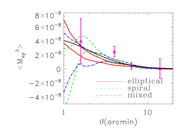
Figure 7: Third order moment of the aperture mass $\langle M_{\rm ap}^{3}\rangle_{\vartheta}$ measured by Jarvis et al. (2004) on the CTIO data (pink triangles) compared with the expected measured third order aperture mass statistics, i.e. GGG+III+GII+GGI, for the three models of galaxies used in this paper. For each model we show a lower and upper value of the total third order moment given by the average $\pm 1\sigma$ error bars. This error is computed as a quadratic sum of the error affecting each term. The GGG weak lensing signal is the same used in Jarvis et al. (2004), i.e. the one for a single source redshift at $z_{\rm s}=0.66$. The III signal has been computed using a galaxy redshift distribution with $z_{\rm l}<0.8$ which is characterized by the similar median redshift $z_{\rm m}\sim 0.66$ used to compute the GGG signal. The GII and GGI terms have been rescaled by using the equations (19) and (21) for a survey with $z_{\rm s}=0.66$ and $z_{\rm l}<0.66$. For comparison we plot the expected weak lensing $\langle M_{\rm ap}^{3}\rangle_{\vartheta}$ (black solid line).

In order to compare our results to observations we present in in Figure 7 the $\langle M_{\rm ap}^{3}\rangle$ results by Jarvis et al. (2004) and the $\langle M_{\rm ap}^{3}\rangle$ that we would expect for this same survey from weak gravitational lensing and the III, GGI and GII terms. For this comparison we have used all of the three galaxy models. We compute the GGG signal using a redshift plane at $z_{\rm s}=0.66$ as done by Jarvis et al. (2004). We add the III model using galaxies with $z<0.8$ so that the redshift distribution is characterized by the a median redshift similar to the one of the CTIO galaxy catalogue. We use Equation (19) and Equation (21) to rescale the GII and GGI to a survey with $z_{\rm s}=0.66$ and $z_{\rm l}<0.66$. For this survey we find that the dominant contribution is given by the GGI which slightly decreases the estimated the weak lensing signal. We find that all three galaxy models are consistent with the Jarvis et al. (2004) results.

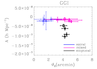
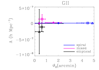
Figure 5: Left panel: best-fit values for the parameters $\vartheta_{0}$ and $A$ of Equation (22) used to fit the angular dependence of GGI for the four redshift distributions; we chose to indicate each source/redshift distribution using the same symbols as Figure 3. Right panel: shows the same parameters as left panel but now for the GII component.

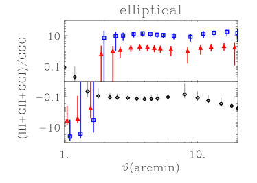
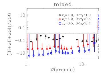
Figure 6: Ratio between the sum of the terms GII, GGI and III and the weak lensing third order moment signal GGG, for the elliptical (left panel) and mixed model (right panel). Three cases are shown: $z_{\rm s}=1$, $0<z_{\rm l}<1$ (black diamonds), $z_{\rm s}=1$, $0<z_{\rm l}<0.4$ (red triangles) and $z_{\rm s}=0.5$, $0<z_{\rm l}<0.4$ (blue squares). For the first and second case the GGG component is computed assuming $z_{\rm s}=1.05$. For the third case $z_{\rm s}=0.45$.

6 Conclusion

Using a set of realistic N-body $\Lambda$CDM simulations we have explored the effect of intrinsic galaxy alignments and the coupling between weak lensing and the foreground ellipticity field on the third order moment of the aperture mass. We find that the intrinsic alignment dominates the three-point shear signal for shallow surveys. For deeper surveys the intrinsic alignment is less significant, as a result of projection effects. Nevertheless, if not taken into account properly, it will still limit the accuracy of tomography measurement and affect the predictions of cosmological values for the next generation of very large surveys, where the signal to noise ratio is high.

We found that for a given survey depth intrinsic alignments affect the three-point weak lensing statistics more strongly than the two-point shear statistics. In other words, in order to achieve the same level of accuracy in the three-point shear statistics measurement as the two-point weak lensing shear statistics one needs deeper surveys.

Overall, this result shows once more the importance of the knowledge of redshift for each individual galaxy for high-precision cosmology. Knowing the redshift of each source allows one to remove the bias from intrinsic galaxy alignments by discarding physically close triplets (pairs) when computing the three-point (two-point) shear statistics. Moreover the knowledge of redshift allows one to model the intrinsic alignment and remove its effect on the two-point weak lensing shear statistics (Joachimi & Schneider, in prep.).

In this perspective, the measurement of the three-point shear statistics from a shallow survey offers a particularly effective way to test intrinsic alignment models. As we showed in this work, the three-point shear statistics in low redshift bins are dominated by the intrinsic alignment term, permitting accurate measurements on intrinsic alignment models. As future dark energy surveys will rely heavily on the good modeling of these effects so they can be marginalised out, this result provides an important new route to constrain and model this physical systematic effect. It is indeed possible to choose low-redshift bins in order to enhance the intrinsic alignment signal so that the shear signal becomes negligible; for example, by selecting galaxies at $z<0.4$. In this case the III/GGG ratio is around fifty, allowing one to study the intrinsic alignment, essentially without contamination from the weak lensing shear.

Using projected mass maps we have studied the shear-shape coupling effect which is also likely to bias the measurement of the third order moment of weak lensing shear. We showed that this systematic can be described by two terms, GGI and GII, which affects the third order moment measurement in a non-trivial way and is dependent on the distance between the lenses and sources and on the morphology of galaxies. Even for a moderately deep survey like the CFHTLS Wide the amplitude of the third order moment of the shear estimation could be underestimated by $\sim 5-10\%$. For shallower surveys such as KIDS or PanSTARRS-1 the bias is expected to be higher. Our results show that it will not be possible to carry out precise three-point cosmic shear measurements with these surveys without modeling the coupling between weak lensing shear and intrinsic alignment. Also for the next generation of deep large surveys, such as SNAP, DUNE or LSST the precision one can achieve on the cosmological constraints relies in the ability to model and marginalize out the shear-shape and intrinsic correlations.

It is possible to use simple models to describe both the angular and redshift dependence of the GGI and GII terms. These models can be used to correct the effect of the coupling between shear and intrinsic alignment on the third order moment of the aperture mass.

Unfortunately, the sample available for this work is not big enough to give a definitive answer; more precisely, the parametric models we used to fit the GGI and GII components are marginally constrained, due to the large statistical and sampling variance affecting our sample. A more detailed study of the redshift dependence of the shear-ellipticity correlation will be required. Such a study should use a larger sample of simulations in order to better constrain our models. Furthermore, we still need to develop a method to include satellite galaxies and account for environmental effects when determining the ellipticity of galaxies in a single parent halo. In addition, an improved mixed galaxy population as a function of redshift evolution would also play an important role in establishing the correct average effects, as we have shown in this paper the net effect depends on the morphology of the galaxy population. We also think that a comparison between results from simulations with results from real data is the best way to validate our results. Concerning this point, the agreement between simulations and real data shown in the study of the II (H06) and GI (Hirata et al. 2007) components is a good indication of the fact that the simulation used in this work, even if it represents a simplified model, shows the correct dependence of the intrinsic alignment effect on morphology of the galaxies, luminosity and redshift.

Like other previous works on intrinsic alignment and shear-shape coupling, this paper demonstrates the great importance of reliable redshifts for future and current galaxies surveys, which could be used, in parallel with simulated catalogues, to study and correct for intrinsic alignment and shear-shape coupling on the two- and three-point weak lensing statistics.

7 Acknowledgments

We thank Alan Heavens and Ismael Tereno for helpful suggestions on this project and Asantha Cooray for making code based on the CLF publicly available. We also would like to thank Martin White for generating the N-body simulations used for this work. These simulations were performed on the IBM-SP at NERSC. ES is supported by the Humboldt Foundation. CH is supported by the European Commission Programme in the framework of a Marie Curie Fellowship under contract MOIF-CT-2006-21891. LW acknowledges support from NSERC and CIAR. This work has been supported by the RTN Network DUEL and the DFG through the TR33 ‘The Dark Universe’ and the project SCHN 342/6–1.

References

- [ Bacon et al. 2003] Bacon D., Refregier A., Ellis R., 2003, MNRAS, 344, 673
- [ Benjamin et al. 2007] Benjamin J., Heymans C., Semboloni E., van Waerbeke L., Hoekstra H., Erben T., Gladders M., Hetterscheidt M., 2007, MNRAS, 381, 702
- [Bernardeau et al. 1999] Bernardeau F., van Waerbeke L., Mellier Y., 1997, A&A, 322, 1
- [Bernardeau et al. 2002] Bernardeau F., Mellier Y., van Waerbeke L., 2002, A&A, 389, 28
- [Bernstein & Jarvis 2002] Bernstein G., Jarvis M., 2002, ApJ, 123,583
- [Bridle & King 2007] Bridle S., King L., 2007, NJPh, 9, 444
- [Brown et al. 2002] Brown M., Taylor A., Hambly N., Dye S., 2002, MNRAS, 333, 501
- [ Brown et al. 2003] Brown M., Taylor A., Bacon D., Gray M., Dye S., Meisenheimer K., Wolf C., 2003, MNRAS, 341, 100
- [Cooray 2006] Cooray A., 2006, MNRAS, 365, 842
- [Cooray & Milosavljevic 2005] Cooray A., Milosavljevic M., 2005, ApJl, 627, L89
- [Crittenden et al. 2001] Crittenden R., Robert G., Natarajan P., Pen U. L., Theuns T., 2001, ApJ, 559, 552
- [Crittenden et al. 2002] Crittenden R., Robert, G., Natarajan P., Pen U. L., Theuns T., 2002, ApJ, 568, 20
- [Fry 1984] Fry J. N., 1984, ApJ, 279, 499
- [Fu et al. 2008] Fu L., Semboloni E., Hoekstra H., Kilbinger M., van Waerbeke L., Tereno I. et al., 2008, A&A, 479, 9
- [Hamana et al. 2003] Hamana T., Miyazaki S., Shimasaku K. et al., 2003, ApJ, 597, 98
- [Heavens et al. 2000] Heavens A., Réfrégier A., Heymans C., 2000, MNRAS, 319, 649
- [Heavens et al. 2007] Heavens A., Kitching T., Taylor A.N., 2006, MNRAS, 373, 105
- [Heymans & Heavens 2003] Heymans C., Heavens A., 2003, MNRAS, 339, 711
- [Heymans et al. 2004] Heymans C., Brown M., Heavens A., Meisenheimer K., Taylor A., 2004, MNRAS, 347, 895
- [Heymans et al. 2005] Heymans C., Brown M., Barden M., Caldwell J., Jahnke K., Rix H., Taylor A., Beckwith S., Bell E., Borch A., Hüsler B., Jogee S., McIntosh D., Meisenheimer K., Peng C., Sanchez S., Somerville R., Wisotzki L., Wolf C., 2005, MNRAS, 160
- [Heymans et al. 2006] Heymans C., White M., Heavens A., Vale C., van Waerbeke L., 2006, MNRAS, 371, 750
- [Hirata & Seljak 2004] Hirata C., Seljak U., 2004, Phys Rev D, 70
- [Hirata et al. 2007] Hirata C., Mandelbaum R., Ishak M., Seljak U., Nichol R., Pimbblet K., Ross N., Wake D., 2007, MNRAS, 38, 1197
- [Hoekstra et al. 2006] Hoekstra H., Mellier Y., van Waerbeke L., Semboloni E., Fu L., Hudson M., Parker L., Tereno I., Benebed K., 2006, ApJ, 347, 116
- [Hoekstra et al. 2002] Hoekstra H., Yee H., Gladders M., 2002, ApJ, 577, 595
- [Jarvis et al. 2003] Jarvis M., Bernstein G., Jain B., Fischer P., Smith D., Tyson J., Wittman D., 2003, ApJ, 552, L21
- [Jarvis et al. 2004] Jarvis M., Bernstein G., Jain B., 2004, MNRAS, 352,338
- [Kaiser et al. 1995] Kaiser N., Squires G., Broadhurst T., 1995, ApJ, 449, 460
- [King & Schneider 2002] King L., Schneider P., 2002, A&A, 396, 411
- [King & Schneider 2003] King L., Schneider P., 2003, A&A, 398, 23
- [King 2005] King L., 2005, A&A, 441, 47
- [ Mandelbaum et al. 2006] Mandelbaum R., Hirata C., Ishak M., Seljak U., Brinkmann J., 2006, MNRAS, 367, 611
- [Kitching et al 2007] Kitching T., Heavens A., Taylor A., Brown M., Meisenheimer K., Wolf C., Gray M., Bacon D., 2007, 376,771
- [Massey et al. 2007] Massey R., Rhodes J., Leauthaud A., Capak P., Ellis R., Koekemoer A., Réfrégier A., Scoville N., Taylor J.E., Albert J., Bergé J., Heymans C., Johnston D., Kneib J.P., Mellier Y., Mobasher B., Semboloni E., Shopbell P., Tasca L., van Waerbeke L., 2007, ApJS, 172, 239
- [Massey et al. 2005] Massey R., Réfrégier A., Bacon D., Ellis R., Brown M., 2005, MNRAS, 359, 1277
- [Pen et al. 2003] Pen U., Zhang T., van Waerbeke L., Mellier Y., Zhang P., Dubinski J., 2003, ApJ, 592, 873
- [Pen et al. 2002] Pen U., van Waerbeke L., Mellier L, 2002, ApJ, 567, 31
- [ Rhodes et al. 2004] Rhodes J., Réfrégier A., Collins N., Gardner J., Groth E., Hill R., 2004, ApJ, 605, 29
- [Rhodes et al. 2000] Rhodes J., Réfrégier A., Groth E., 2000, ApJ, 536, 79
- [ Semboloni et al. 2006] Semboloni E., Mellier Y., van Waerbeke L., Hoekstra H., Tereno I., Benabed K., Gwyn S., Fu L., Hudson M., Maoli R., Parker L., 2006, A&A, 452, 51
- [Schneider et al. 2005] Schneider P., Kilbinger M., Lombardi M., 2005, A&A, 431, 9
- [Schneider & Lombardi 2003] Schneider P., Lombardi M., 2003, A&A, 408, 829
- [Schneider et al. 2002] Schneider P., van Waerbeke L., Kilbinger M., Mellier Y., 2002, A&A , 396,1
- [Scoccimarro & Couchman 2001] Scoccimarro R., Couchman H.M.P., 2001, MNRAS, 325, 1312
- [van den Bosch et al. 2002] van den Bosch F. C., Abel T., Croft R. A. C., Hernquist L., White S. D. M., 2002, ApJ, 576, 699
- [Schneider et al. 1998] Schneider P., van Waerbeke L., Jain B., Kruse G., 1998, MNRAS, 296,873
- [van Waerbeke et al. 2005] van Waerbeke L., Mellier Y., Hoekstra H., 2005, A&A, 429, 75
- [van Waerbeke et al. 2001] van Waerbeke L., Mellier Y., Radovich M., Bertin E., Dantel-Fort M., McCracken H., Le Fèvre O., Foucaud S., Cuillandre J., Erben T., Jain B., Schneider P., Bernardeau F., Fort B., 2001, A&A, 347, 757
- [Zhang & Pen 2004] Zhang L., Pen U., 2005, New Astronomy, 10, 569