CERN-PH-TH/2008-041

ITP–UH–04/08

LMP-TPU–01/08

N=4 mechanics, WDVV equations and roots
$\textrm{\Large Anton Galajinsky\ }^{a},\quad\textrm{\Large Olaf Lechtenfeld\ }^{b\ c},\quad\textrm{\Large Kirill Polovnikov\ }^{a}$
^a Laboratory of Mathematical Physics, Tomsk Polytechnic University,
634050 Tomsk, Lenin Ave. 30, Russian Federation

Emails: galajin, kir @mph.phtd.tpu.edu.ru
^b Theory Division, Physics Department, CERN,
1211 Geneva 23, Switzerland

Email: olaf.lechtenfeld@cern.ch
^c Institut für Theoretische Physik, Leibniz Universität Hannover,
Appelstrasse 2, D-30167 Hannover, Germany

Email: lechtenf@itp.uni-hannover.de

${\cal N}{=}4$ superconformal multi-particle quantum mechanics on the real line is governed by two prepotentials, $U$ and $F$, which obey a system of partial differential equations linear in $U$ and generalizing the Witten-Dijkgraaf-Verlinde-Verlinde (WDVV) equation for $F$. Putting $U{\equiv}0$ yields a class of models (with zero central charge) which are encoded by the finite Coxeter root systems. We extend these WDVV solutions $F$ in two ways: the $A_{n}$ system is deformed $n$-parametrically to the edge set of a general orthocentric $n$-simplex, and the $BCF$-type systems form one-parameter families. A classification strategy is proposed. A nonzero central charge requires turning on $U$ in a given $F$ background, which we show is outside the reach of the standard root-system ansatz for indecomposable systems of more than three particles. In the three-body case, however, this ansatz can be generalized to establish a series of nontrivial models based on the dihedral groups $I_{2}(p)$, which are permutation symmetric if 3 divides $p$. We explicitly present their full prepotentials.

1 Introduction

It has been known for a long time that integrable quantum systems are intimately related to Lie algebras (see, for instance, [1]). Therefore, it is natural to expect their appearance also in supersymmetric extensions of integrable multi-particle quantum mechanics models. In this paper, we revisit such systems with ${\cal N}{=}4$ superconformal symmetry in one space dimension and, within a canonical ansatz, investigate them for the superconformal algebra $su(1,1|2)$ with central charge $C$. Despite physical interest in these models [2], their explicit construction has remained an open problem until now.

${\cal N}{=}4$ superconformal many-body quantum systems on the real line are very rigid. Their existence is governed by a system of nonlinear partial differential equations for two prepotentials, $U$ and $F$, for which few solutions are known when $C{\neq}0$ [3, 4, 5, 6]. The determination of $F$ is decoupled from $U$ and requires solving ‘only’ the well-known (generalized) Witten-Dijkgraaf-Verlinde-Verlinde (WDVV) equation [7, 8], which arises in topological and Seiberg-Witten field theory. The WDVV solutions known so far are all based – again – on the root systems of simple Lie algebras [9, 10].

If $C{=}0$ any WDVV solution $F$, together with $U{\equiv}0$, will provide a valid multi-particle quantum model. For nonzero central charge, however, one is to solve a second partial differential equation for $U$ in the presence of $F$. To this so-called ‘flatness conditon’ only particular solutions for at most four particles are in the literature [3, 6].

All considerations up to now have employed a natural ansatz for $F$ and $U$ in terms of a set $\{\alpha\}$ of covectors. We find, however, that for systems of less than four particles this ansatz must be generalized in order to capture all solutions. In these cases, the WDVV equation is trivially satisfied, and we can (and do) construct new three-body models for any dihedral $I_{2}(p)$ root system, starting with a Calogero-type $A_{2}$ model. For more than three particles, where the WDVV equation is effective, we show that even our generalized ansatz is insufficient to produce irreducible $U{\neq}0$ solutions in the root-system context. A model is reducible if, after removing the center-of-mass degree of freedom, it can be decomposed into decoupled subsystems. As for the WDVV equation alone, we generalize the solutions of [9, 10] and give a geometric interpretation of certain $A_{n}$ deformations [11] in terms of orthocentric simplices.

The paper is organized as follows. In Section 2 we recall the formulation of conformal mechanics of $n{+}1$ identical particles on the real line in terms of $so(1,2)$ generators including the Hamiltonian. In this description, an ${\cal N}{=}4$ supersymmetric extension with central charge $C$ is straightforward to construct as we demonstrate in Section 3. The closure of the superconformal algebra poses constraints on the interaction, which in Section 4 lead to what we call the ‘structure equations’ on the prepotentials $U$ and $F$. The analysis of these structure equations in Section 5 suggests constructing the prepotentials in terms of a system of covectors, which reduces the differential equations to nonlinear algebraic equations. Sections 6 and 7 derive families of $F$ solutions with $U{\equiv}0$, based on certain deformations of the root systems of the finite reflection groups. Turning on $U$ for these $F$ backgrounds is analyzed in Sections 8 and 9, with negative results for more than three particles, but with a positive classification and the full construction of the prepotentials for three particles via the dihedral groups $I_{2}(p)$, including five explicit examples. Section 10 concludes.

2 Conformal quantum mechanics

Let us consider a system of $n{+}1$ identical particles with unit mass, moving on the real line according to a Hamiltonian of the generic form ($I=1,\ldots,n{+}1$)

$$H\ =\ {\textstyle\frac{1}{2}}p_{I}p_{I}\ +\ V_{B}(x^{1},\dots,x^{n+1})\ .$$ (2.1)

Throughout the paper a summation over repeated indices is understood. After separating the center-of-mass motion we will work with the $n$ degrees of freedom of relative particle motion in later sections. Also, the bosonic potential $V_{B}$ will get supersymmetrically extended to a potential $V$ including $V_{B}$.

For conformally invariant models the Hamiltonian $H$ is a part of the $so(1,2)$ conformal algebra

$$[D,H]\ =\ -{\rm i}H\ ,\quad[H,K]\ =\ 2{\rm i}D\ ,\quad[D,K]\ =\ {\rm i}K\ ,$$ (2.2)

where $D$ and $K$ are the dilatation and conformal boost generators, respectively. Their realization in term of coordinates and momenta, subject to

$$[x^{I},p_{J}]\ =\ {\rm i}{\delta_{J}}^{I}\ ,$$ (2.3)

reads

$$D\ =\ -{\textstyle\frac{1}{4}}(x^{I}p_{I}+p_{I}x^{I})\qquad\textrm{and}\qquad K\ =\ {\textstyle\frac{1}{2}}x^{I}x^{I}\ .$$ (2.4)

The first relation in (2.2) restricts the potential via

$$(x^{I}\partial_{I}+2)\,V_{B}\ =\ 0\ ,$$ (2.5)

meaning that $V_{B}$ must be homogeneous of degree $-2$ for the model to be conformally invariant. Imposing translation and permutation invariance and allowing only two-body interactions, we arrive at the Calogero model of $n{+}1$ particles interacting through an inverse-square pair potential,

$$V_{B}\ =\ \sum_{I<J}{\textstyle\frac{g^{2}}{(x^{I}-x^{J})^{2}}}\qquad\longrightarrow\qquad H\ =\ H_{0}\ +\ V_{B}\ .$$ (2.6)

3 N=4 superconformal extension

Let us extend the bosonic conformal mechanics of the previous section to an ${\cal N}{=}4$ superconformal one,  with a single central extension [13]. The bosonic sector of the ${\cal N}{=}4$ superconformal algebra $su(1,1|2)$ includes two subalgebras. Along with $so(1,2)$ considered in the previous section one also finds the $su(2)$ R-symmetry subalgebra generated by $J_{a}$ with $a=1,2,3$. The fermionic sector is exhausted by the SU(2) doublet supersymmetry generators $Q_{\alpha}$ and ${\bar{Q}}^{\alpha}$ as well as their superconformal partners $S_{\alpha}$ and ${\bar{S}}^{\alpha}$, with $\alpha=1,2$, subject to the hermiticity relations

$${(Q_{\alpha})}^{\dagger}\ =\ {\bar{Q}}^{\alpha}\qquad\textrm{and}\qquad{(S_{\alpha})}^{\dagger}\ =\ {\bar{S}}^{\alpha}\ .$$ (3.1)

The bosonic generators are hermitian. The non-vanishing (anti)commutation relations in our superconformal algebra read

$$[D,H]\ =\ -{\rm i}\,H\ , [H,K]\ =\ 2{\rm i}\,D\ ,$$

$$[D,K]\ =\ +{\rm i}\,K\ , [J_{a},J_{b}]\ =\ {\rm i}\,\epsilon_{abc}J_{c}\ ,$$

$$\{Q_{\alpha},\bar{Q}^{\beta}\}\ =\ 2\,H{\delta_{\alpha}}^{\beta}\ , \{Q_{\alpha},\bar{S}^{\beta}\}\ =\ +2{\rm i}\,{{(\sigma_{a})}_{\alpha}}^{\beta}J_{a}-2\,D{\delta_{\alpha}}^{\beta}-{\rm i}\,C{\delta_{\alpha}}^{\beta}\ ,$$

$$\{S_{\alpha}\,,\,\bar{S}^{\beta}\}\ =\ 2\,K{\delta_{\alpha}}^{\beta}\ , \{\bar{Q}^{\alpha},S_{\beta}\}\ =\ -2{\rm i}\,{{(\sigma_{a})}_{\beta}}^{\alpha}J_{a}-2\,D{\delta_{\beta}}^{\alpha}+{\rm i}\,C{\delta_{\beta}}^{\alpha}\ ,$$

$$[D,Q_{\alpha}]\ =\ -{\textstyle\frac{1}{2}}{\rm i}\,Q_{\alpha}\ , [D,S_{\alpha}]\ =\ +{\textstyle\frac{1}{2}}{\rm i}\,S_{\alpha}\ ,$$

$$[K,Q_{\alpha}]\ =\ +{\rm i}\,S_{\alpha}\ , [H,S_{\alpha}]\ =\ -{\rm i}\,Q_{\alpha}\ ,$$

$$[J_{a},Q_{\alpha}]\ =\ -{\textstyle\frac{1}{2}}\,{{(\sigma_{a})}_{\alpha}}^{\beta}Q_{\beta}\ , [J_{a},S_{\alpha}]\ =\ -{\textstyle\frac{1}{2}}\,{{(\sigma_{a})}_{\alpha}}^{\beta}S_{\beta}\ ,$$

$$[D,\bar{Q}^{\alpha}]\ =\ -{\textstyle\frac{1}{2}}{\rm i}\,\bar{Q}^{\alpha}\ , [D,\bar{S}^{\alpha}]\ =\ +{\textstyle\frac{1}{2}}{\rm i}\,\bar{S}^{\alpha}\ ,$$

$$[K,\bar{Q}^{\alpha}]\ =\ +{\rm i}\,\bar{S}^{\alpha}\ , [H,\bar{S}^{\alpha}]\ =\ -{\rm i}\,\bar{Q}^{\alpha}\ ,$$

$$[J_{a},\bar{Q}^{\alpha}]\ =\ {\textstyle\frac{1}{2}}\,\bar{Q}^{\beta}{{(\sigma_{a})}_{\beta}}^{\alpha}\ , [J_{a},\bar{S}^{\alpha}]\ =\ {\textstyle\frac{1}{2}}\,\bar{S}^{\beta}{{(\sigma_{a})}_{\beta}}^{\alpha}\ .$$ (3.2)

Here $\epsilon_{123}=1$, and $C$ stands for the central charge.

For a mechanical realization of the $su(1,1|2)$ superalgebra, one introduces fermionic degrees of freedom represented by the operators $\psi^{I}_{\alpha}$ and $\bar{\psi}^{I\alpha}$, with $I=1,\dots,n{+}1$ and $\alpha=1,2$, which are hermitian conjugates of each other and obey the anti-commutation relations

$$\{\psi^{I}_{\alpha},\psi^{J}_{\beta}\}\ =\ 0\ ,\qquad\{{\bar{\psi}}^{I\alpha},{\bar{\psi}}^{J\beta}\}\ =\ 0\ ,\qquad\{\psi^{I}_{\alpha},{\bar{\psi}}^{J\beta}\}\ =\ \,{\delta_{\alpha}}^{\beta}\delta^{IJ}\ .$$ (3.3)

In the extended space it is easy to construct the free fermionic generators associated with the free Hamiltonian $H_{0}=\frac{1}{2}p_{I}p_{I}$, namely

$${Q_{0}}_{\alpha}\ =\ p_{I}\psi^{I}_{\alpha}\ ,\qquad\bar{Q}_{0}^{\alpha}\ =\ p_{I}\bar{\psi}^{I\alpha}\qquad\textrm{and}\qquad{S_{0}}_{\alpha}\ =\ x^{I}\psi^{I}_{\alpha}\ ,\qquad\bar{S}_{0}^{\alpha}\ =\ x^{I}\bar{\psi}^{I\alpha}\ ,$$ (3.4)

as well as $su(2)$ generators

$${J_{0}}_{a}\ =\ {\textstyle\frac{1}{2}}\bar{\psi}^{I\alpha}{{(\sigma_{a})}_{\alpha}}^{\beta}\psi^{I}_{\beta}\ .$$ (3.5)

Notice that these are automatically Weyl-ordered. The free dilatation and conformal boost operators maintain their bosonic form

$$D_{0}\ =\ -{\textstyle\frac{1}{4}}(x^{I}p_{I}+p_{I}x^{I})\qquad\textrm{and}\qquad K_{0}\ =\ {\textstyle\frac{1}{2}}x^{I}x^{I}\ .$$ (3.6)

In contrast to the ${\cal N}{\leq}2$ cases, the free generators fail to satisfy the full algebra (3). Even for $C{=}0$, the $\{Q,\bar{S}\}$ and $\{\bar{Q},S\}$ anticommutators require corrections to the fermionic generators, which are cubic in the fermions and can be restricted to $Q$ and $\bar{Q}$ via

$$Q_{\alpha}\ =\ Q_{0\alpha}-{\rm i}\,[S_{0\alpha},V]\qquad\textrm{and}\qquad\bar{Q}^{\alpha}\ =\ \bar{Q}^{\alpha}_{0}-{\rm i}\,[\bar{S}^{\alpha}_{0},V]\qquad\textrm{where}\quad H\ =\ H_{0}+V$$ (3.7)

and $V\neq 0$. Hence, there does not exist a free mechanical representation of the algebra (3). It follows further that $V$ contains terms quadratic and quartic in the fermions, thus can be written as [3, 5, 6]

$$V\ =\ V_{B}(x)\ -\ U_{IJ}(x)\langle\psi^{I}_{\alpha}{\bar{\psi}}^{J\alpha}\rangle\ +\ {\textstyle\frac{1}{4}}F_{IJKL}(x)\langle\psi^{I}_{\alpha}\psi^{J\alpha}\bar{\psi}^{K\beta}\bar{\psi}^{L}_{\beta}\rangle\ ,$$ (3.8)

with completely symmetric unknown functions $U_{IJ}$ and $F_{IJKL}$ homogeneous of degree $-2$ in $x\equiv\{x^{1},\ldots,x^{n+1}\}$. Here, the symbol $\langle\dots\rangle$ stands for symmetric (or Weyl) ordering. The ordering ambiguity present in the fermionic sector affects the bosonic potential $V_{B}$. In contrast to the ${\cal N}{=}2$ superconformal extensions [14, 15], the quartic term is needed, and so we get

$$Q_{\alpha} \ =\ \bigl{(}p_{J}-{\rm i}\,x^{I}\,U_{IJ}(x)\bigr{)}\,\psi_{\alpha}^{J}\ \,-{\textstyle\frac{{\rm i}}{2}}\,x^{I}\,F_{IJKL}(x)\,\langle\psi^{J}_{\beta}\,\psi^{K\beta}\bar{\psi}^{L}_{\alpha}\rangle\ ,$$ (3.9)

$$\bar{Q}^{\alpha} \ =\ \bigl{(}p_{J}+{\rm i}\,x^{I}\,U_{IJ}(x)\bigr{)}\,\bar{\psi}^{J\alpha}\,-{\textstyle\frac{{\rm i}}{2}}\,x^{I}\,F_{IJKL}(x)\,\langle\psi^{J\alpha}\bar{\psi}^{K\beta}\bar{\psi}^{L}_{\beta}\rangle\ .$$

To summarize, in order to close the algebra (3), the $D$, $K$, $J_{a}$, $S_{\alpha}$ and $\bar{S}^{\alpha}$ generators remain free, while $Q_{\alpha}$ and $\bar{Q}^{\alpha}$ as well as $H$ acquire corrections as above.

4 The structure equations

Inserting the form (3.4)–(3.8) into the algebra (3), one produces a fairly long list of constraints on the potential $V$. One of the consequences is that [3, 5, 6]

$$U_{IJ}\ =\ \partial_{I}\partial_{J}U\qquad\textrm{and}\qquad F_{IJKL}\ =\ \partial_{I}\partial_{J}\partial_{K}\partial_{L}F\ ,$$ (4.1)

which introduces two scalar prepotentials. The constraints then turn into the following system of nonlinear partial differential equations [5, 6],

$$(\partial_{I}\partial_{K}\partial_{P}F)(\partial_{J}\partial_{L}\partial_{P}F)\ =\ (\partial_{J}\partial_{K}\partial_{P}F)(\partial_{I}\partial_{L}\partial_{P}F)\quad,\qquad x^{I}\partial_{I}\partial_{J}\partial_{K}F\ =\ -\delta_{JK}\ ,$$ (4.2)

$$\partial_{I}\partial_{J}U-(\partial_{I}\partial_{J}\partial_{K}F)\,\partial_{K}U\ =\ 0\quad,\qquad\qquad\qquad\qquad\qquad x^{I}\partial_{I}U\ =\ -C\ ,\qquad\quad{}$$ (4.3)

which we refer to as the ‘structure equations’. Notice that these equations are quadratic in $F$ but only linear in $U$. They are invariant under SO($n{+}1$) coordinate transformations. The first of (4.2) is a kind of zero-curvature condition for a connection $\partial^{3}F$. It coincides with the (generalized) WDVV equation known from topological field theory [7, 8]. The first of (4.3) is a kind of covariant constancy for $\partial U$ in the $\partial^{3}F$ background. Since its integrability implies the WDVV equation projected onto $\partial U$, we call it the ‘flatness condition’.

The right equations in (4.2) and (4.3) represent homogeneity conditions for $U$ and $F$. They are inhomogeneous with constants $\delta_{jk}$ and $C$ (the central charge) on the right-hand side and display an explicit coordinate dependence. Furthermore, the second equation in (4.2) can be integrated twice to obtain

$$x^{I}\partial_{I}F-2F+{\textstyle\frac{1}{2}}x^{I}x^{I}\ =\ 0\ ,$$ (4.4)

where we used the freedom in the definition of $F$ to put the integration constants – a linear function on the right-hand side – to zero. It is important to realize that the inhomogeneous term in this integrated equation excludes the trivial solution $F=0$ equivalent to a homogeneous quadratic polynomial. This effect is absent in ${\cal N}{=}2$ superconformal models, where the four-fermion potential term is not required and, hence, $F$ need not appear [15]. This issue is also discussed in [3].

To simplify the analysis of the structure equations, it is convenient to separate the center-of-mass and the relative motion of the particles. This is achieved by a rotation of the coordinate frame,

$$\{\,x^{I}\,\}\ \longrightarrow\ \{\,x^{i}\,,\,X\,\}\qquad\textrm{with}\qquad i=1,\ldots,n\qquad\textrm{and}\qquad X\ =\ {\textstyle\frac{1}{\sqrt{n+1}}}\,{\textstyle\sum}_{I=1}^{n+1}\,x^{I}\ ,$$ (4.5)

which introduces relative-motion coordinates $x^{i}$ for the hyperplane orthogonal to the center-of-mass direction. The structure equations then hold for both sets of coordinates independently, with an accompanying split of the prepotentials and the central charge,

$$F\ =\ F_{\text{com}}(X)+F_{\text{rel}}(x)\ ,\qquad U\ =\ U_{\text{com}}(X)+U_{\text{rel}}(x)\qquad\textrm{and}\qquad C\ =\ C_{\text{com}}+C_{\text{rel}}\ ,$$ (4.6)

where now $x\equiv\{x^{i}\}$. For the center-of-mass coordinate, the solution is trivial:

$$F_{\text{com}}\ =\ -{\textstyle\frac{1}{2}}\,X^{2}\,\ln|X|\qquad\textrm{and}\qquad U_{\text{com}}\ =\ -C_{\text{com}}\,\ln|X|\ .$$ (4.7)

For the relative coordinates, we simply replace $I,J,\ldots$ by $i,j,\ldots$ and $C\to C_{\text{rel}}$ in the structure equations. In the following, we shall investigate the construction of $F_{\text{rel}}$ and $U_{\text{rel}}$ only and therefore drop the label ‘rel’ from now on. However, since these coordinates often obscure a permutation invariance for identical particles, it can be useful to go back to the original $x^{I}$ by embedding $\mathbb{R}^{n}$ into $\mathbb{R}^{n+1}$ as the hyperplane orthogonal to the vector $\rho={\textstyle\frac{1}{\sqrt{n+1}}}(1,1,\ldots,1)$ for achieving a manifestly permutation-symmetric description of the $(n{+}1)$-particle system. Furthermore, the center-of-mass case is still covered in our analysis by just taking $n{=}1$.

There are some dependencies among the equations (4.2) and (4.3), now reduced to the relative coordinates. The contraction of two left equations with $x^{i}$ is a consequence of the two right equations, and therefore only the components orthogonal to $x$ are independent, effectively reducing the dimension to $n{-}1$. This means that only ${\textstyle\frac{1}{12}}n(n{-}1)^{2}(n{-}2)$ WDVV equations need to be solved and only ${\textstyle\frac{1}{2}}n(n{-}1)$ flatness conditions have to be checked. For $n{=}2$ in particular, the single WDVV equation follows from the homogeneity condition in (4.2), and the three flatness conditions are all equivalent. Hence, the nonlinearity of the structure equations becomes relevant only for $n{\geq}3$.

The scalars $U$ and $F$ govern the ${\cal N}{=}4$ superconformal extension. Note, however, that $F$ is defined modulo a quadratic polynomial while $U$ is defined up to a constant. Together, they determine $V_{B}$ as

$$V_{B}\ =\ {\textstyle\frac{1}{2}}\,(\partial_{i}U)(\partial_{i}U)\ +\ {\textstyle\frac{\hbar^{2}}{8}}\,(\partial_{i}\partial_{j}\partial_{k}F)(\partial_{i}\partial_{j}\partial_{k}F)\ .$$ (4.8)

We note that $U{\equiv}0$ still yields nontrivial quantum models, whose potential only vanishes classically. Finally, from the two right equations in (4.2) and (4.3) it follows that

$$x^{i}\,F_{ijkl}\ =\ -\partial_{j}\partial_{k}\partial_{l}F\qquad\textrm{and}\qquad x^{i}\,U_{ij}\ =\ -\partial_{j}U\ ,$$ (4.9)

which is relevant for (3.9).

5 Prepotential ansatz and consequences

Our attack on (4.2) and (4.3) begins with the homogeneity conditions

$$(x^{i}\partial_{i}-2)F\ =\ -{\textstyle\frac{1}{2}}\,x^{i}x^{i}\qquad\textrm{and}\qquad x^{i}\partial_{i}U\ =\ -C\ .$$ (5.1)

The general solution to (5.1) may be written as

$$F\ =\ -{\textstyle\frac{1}{4}}\sum_{s}f_{s}\ Q_{s}(x)\,\ln|Q_{s}(x)|\ +\ F_{\rm hom}\qquad\textrm{and}\qquad U\ =\ -{\textstyle\frac{1}{2}}\sum_{s}g_{s}\,\ln|Q_{s}(x)|\ +\ U_{\rm hom}$$ (5.2)

with quadratic forms $Q_{s}(x)$, real coefficients $f_{s}$ and $g_{s}$, as well as homogeneous functions $F_{\rm hom}$ and $U_{\rm hom}$ of degree two and zero, respectively. The conditions (5.1) are obeyed if

$$Q_{s}(x)=\sum_{i,j}q^{s}_{ij}\,x^{i}x^{j}\qquad\textrm{satisfies}\qquad\sum_{s}f_{s}\,Q_{s}(x)=x^{i}x^{i}\quad\textrm{and}\quad\sum_{s}g_{s}=C\ .$$ (5.3)

Unfortunately, it is hard to analyze the WDVV equation (4.2) and the flatness condition (4.3) in this generality. Therefore, we take the simplifying ansatz that the quadratic forms are either of rank one or proportional to the identity form,

$$Q_{\alpha}(x)\ =\ \alpha_{i}\alpha_{j}\,x^{i}x^{j}\ =:\ (\alpha{\cdot}x)^{2}\qquad\textrm{and}\qquad Q_{R}(x)\ =\ x^{i}x^{i}\ =:\ R^{2}\ ,$$ (5.4)

which defines a set $\{\alpha\}$ of $p$ covectors

$$\alpha\ =\ (\alpha_{1},\alpha_{2},\ldots,\alpha_{n})\qquad\textrm{with values}\qquad\alpha(x)\ =\ \alpha{\cdot}x\ =\ \alpha_{i}x^{i}\ .$$ (5.5)

Replacing the label ‘$s$’ by the covector name ‘$\alpha$’ or by ‘$R$’, the prepotentials (5.2) read

$$F \ =\ -{\textstyle\frac{1}{2}}\sum_{\alpha}f_{\alpha}\ (\alpha{\cdot}x)^{2}\,\ln|\alpha{\cdot}x|\ -\ {\textstyle\frac{1}{2}}f_{R}\,R^{2}\,\ln R\ +\ F_{\rm hom}(x)\ ,$$ (5.6)

$$U \ =\ -\sum_{\alpha}g_{\alpha}\,\ln|\alpha{\cdot}x|\ -\ g_{R}\,\ln R\ +\ U_{\rm hom}(x)\ .$$

The covector part of this ansatz is well known [3, 6, 9, 10], but the ‘radial’ terms (labelled ‘$R$’) are new and will be important for admitting nontrivial solutions $U$.

The expressions above are invariant under individual sign flips $\alpha\to-\alpha$ for each covector, and so we exclude $-\alpha$ from the set. For identical particles our relative configuration space carries an $n$-dimensional representation of the permutation group ${\cal S}_{n+1}$, whose action must leave the set $\{\pm\alpha\}$ invariant. Furthermore, the $f_{\alpha}$ and $g_{\alpha}$ couplings have to be constant along each ${\cal S}_{n+1}$ orbit. Finally, a rescaling of $\alpha{\cdot}x$ may be absorbed into a renormalization of $f_{\alpha}$. Therefore, only the rays $\mathbb{R}_{+}\alpha$ are invariant data. We cannot, however, change the sign of $f_{\alpha}$ in this manner.

Compatibility of (5.6) with the conditions (5.1) directly yields

$$\sum_{\alpha}f_{\alpha}\,\alpha_{i}\alpha_{j}\ +\ f_{R}\,\delta_{ij}\ =\ \delta_{ij}\qquad\textrm{and}\qquad\sum_{\alpha}g_{\alpha}\ +\ g_{R}\ =\ C\ .$$ (5.7)

The second relation fixes the central charge, and the $g_{\alpha}$ are independent free couplings if not forced to zero. The first relation amounts to a decomposition of $(1{-}f_{R})\delta_{ij}$ into (usually non-orthogonal) rank-one projectors and imposes ${\textstyle\frac{1}{2}}n(n{+}1)$ relations on the coefficients $\{f_{\alpha},f_{R}\}$ for a given set $\{\alpha\}$.

All known solutions to the WDVV equations can be cast into the form (5.6) with $F_{\rm hom}\equiv 0$, so from now on we drop this term. From (5.6) we then derive

$$\partial_{i}\partial_{j}\partial_{k}F \ =\ -\sum_{\alpha}f_{\alpha}\,\frac{\alpha_{i}\alpha_{j}\alpha_{k}}{\alpha{\cdot}x}\ -\ f_{R}\,\Bigl{\{}\frac{x_{i}\delta_{jk}+x_{j}\delta_{ki}+x_{k}\delta_{ij}}{R^{2}}-2\frac{x_{i}x_{j}x_{k}}{R^{4}}\Bigr{\}}\ ,$$ (5.8)

$$\partial_{i}U \ =\ -\sum_{\alpha}g_{\alpha}\,\frac{\alpha_{i}}{\alpha{\cdot}x}\ -\ g_{R}\,\frac{x_{i}}{R^{2}}\ +\ \partial_{i}U_{\rm hom}\ ,$$

and so the bosonic part of the potential takes the form

$$V_{B}\ = {\textstyle\frac{1}{2}}\sum_{\alpha,\beta}\frac{\alpha{\cdot}\beta}{\alpha{\cdot}x\;\beta{\cdot}x}\,\Bigl{(}g_{\alpha}g_{\beta}+{\textstyle\frac{\hbar^{2}}{4}}f_{\alpha}f_{\beta}\,(\alpha{\cdot}\beta)^{2}\Bigr{)}\ -\ \sum_{\alpha}g_{\alpha}\,\frac{\alpha_{i}}{\alpha{\cdot}x}\,\partial_{i}U_{\rm hom}$$ (5.9)

$$+\ {\textstyle\frac{1}{2}}\,\frac{1}{R^{2}}\Bigl{(}g_{R}(2C{-}g_{R})+{\textstyle\frac{\hbar^{2}}{4}}(3n{-}2)f_{R}(2{-}f_{R})\Bigr{)}\ +\ {\textstyle\frac{1}{2}}(\partial_{i}U_{\rm hom})(\partial_{i}U_{\rm hom})\ .$$

The WDVV equation in (4.2) becomes

$${\textstyle\frac{1}{2}}\sum_{\alpha,\beta}f_{\alpha}f_{\beta}\,\frac{\alpha{\cdot}\beta}{\alpha{\cdot}x\,\beta{\cdot}x}\,(\alpha\wedge\beta)^{\otimes 2}\ +\ f_{R}\,(2{-}f_{R})\,\frac{T}{R^{2}}\ =\ 0$$ (5.10)

$$\textrm{with}\qquad(\alpha\wedge\beta)^{\otimes 2}_{ijkl}\ =\ (\alpha_{i}\beta_{j}-\alpha_{j}\beta_{i})(\alpha_{k}\beta_{l}-\alpha_{l}\beta_{k})\qquad\textrm{and}\qquad$$ (5.11)

$$T_{ijkl}\ =\ \delta_{ik}\delta_{jl}-\delta_{il}\delta_{jk}-\delta_{ik}\hat{x}_{j}\hat{x}_{l}+\delta_{il}\hat{x}_{j}\hat{x}_{k}-\delta_{jl}\hat{x}_{i}\hat{x}_{k}+\delta_{jk}\hat{x}_{i}\hat{x}_{l}\quad\textrm{where}\quad\hat{x}_{i}\equiv{\textstyle\frac{x_{i}}{R}}\ .$$

The different singular loci of the various terms in (5.10) allow one to separate them, thus

$$\smash{\sum_{\alpha,\beta\atop(\alpha\neq\beta)}}\!f_{\alpha}f_{\beta}\,\frac{\alpha{\cdot}\beta}{\alpha{\cdot}x\,\beta{\cdot}x}\,(\alpha\wedge\beta)^{\otimes 2}\ =\ 0\qquad\textrm{and}\qquad f_{R}\,(2{-}f_{R})\ =\ 0\ .$$ (5.12)

The two admissible choices for $f_{R}$,

$$f_{R}=0\quad{\buildrel(\ref{hcond})\over{\longrightarrow}}\quad\sum_{\alpha}f_{\alpha}\alpha{\otimes}\alpha=\mathbbm{1}\qquad\textrm{or}\qquad f_{R}=2\quad{\buildrel(\ref{hcond})\over{\longrightarrow}}\quad\sum_{\alpha}f_{\alpha}\alpha{\otimes}\alpha=-\mathbbm{1}\ ,$$ (5.13)

are related by flipping the signs of all coefficients $f_{\alpha}$, i.e. $f_{\alpha}\to-f_{\alpha}$. Note, however, that the $n{=}2$ case is special, since then $T{\equiv}0$ and (5.10) is identically satisfied, so no restrictions on $f_{R}$ arise.

The flatness condition in (4.3), on the other hand, is already nontrivial at $n{=}2$ and reads

$$\partial_{i}\partial_{j}U\ +\ \sum_{\alpha}f_{\alpha}\frac{\alpha_{i}\alpha_{j}}{\alpha{\cdot}x}\,\alpha{\cdot}\partial U\ +\ f_{R}\,\Bigl{\{}\frac{x_{i}\partial_{j}U+x_{j}\partial_{i}U-\delta_{ij}C}{R^{2}}+\frac{2x_{i}x_{j}C}{R^{4}}\Bigr{\}}\ =\ 0\ .$$ (5.14)

In particular, its trace,

$$\partial{\cdot}\partial\,U\ +\ \sum_{\alpha}f_{\alpha}\frac{\alpha{\cdot}\alpha}{\alpha{\cdot}x}\alpha{\cdot}\partial U\ =\ C\,f_{R}\,\frac{n}{R^{2}}\ ,$$ (5.15)

and its projection onto some covector $\beta$,

$$(\beta{\cdot}\partial)^{2}U\ +\ \sum_{\alpha}f_{\alpha}\frac{(\alpha{\cdot}\beta)^{2}}{\alpha{\cdot}x}\alpha{\cdot}\partial U\ +\ 2f_{R}\frac{\beta{\cdot}x}{R^{2}}\,\beta{\cdot}\partial U\ =\ C\,f_{R}\Bigl{(}\frac{\beta{\cdot}\beta}{R^{2}}-\frac{2(\beta{\cdot}x)^{2}}{R^{4}}\Bigr{)}\ ,$$ (5.16)

prove to be useful. They are potentially singular at $R{=}0$ and on the hyperplanes $\alpha{\cdot}x{=}0$. For example, near $\beta{\cdot}x{=}0$ (but away from $R{=}0$) we may approximate (5.16) by

$$(\beta{\cdot}\partial)^{2}U\ +\ \frac{f_{\beta}\,\beta{\cdot}\beta}{\beta{\cdot}x}\,\beta{\cdot}\partial U\ \approx\ 0\qquad{\buildrel f_{\beta}\geq-1\over{\longrightarrow}}\qquad U\ \sim\ (\beta{\cdot}x)^{1-f_{\beta}}\quad\textrm{for}\quad\beta{\cdot}x\sim 0\ ,$$ (5.17)

which displays the leading singularity structure of $U$ (and thus of $V_{B}$) on the $\beta{\cdot}x{=}0$ hyperplane provided that $f_{\beta}$ is sufficiently large.

Of course, there is always the trivial $C{=}0$ solution, which puts $g_{R}=g_{\alpha}=0\ \ \forall\alpha$. As long as we keep $U_{\rm hom}$ to be nonzero, it is not too illuminating to insert the covector expression (5.8) into the above equations. So let us, for a moment, ponder the consequences of putting $U_{\rm hom}\equiv 0$ in (5.6). In such a case for $n{>}2$, (5.14) together with (5.8) implies

$$g_{\alpha}\,(1{-}\alpha{\cdot}\alpha f_{\alpha})\ =\ 0\ ,\quad\smash{\sum_{\alpha,\beta\atop(\alpha\neq\beta)}}\!g_{\alpha}f_{\beta}\,\frac{\alpha{\cdot}\beta\ \beta_{i}\beta_{j}}{\alpha{\cdot}x\ \beta{\cdot}x}\ =\ 0\ ,\quad g_{\alpha}\,f_{R}\ =\ C\,f_{R}\ =\ g_{R}\ =\ 0\ ,$$ (5.18)

which essentially kills all radial terms and fixes $f_{\alpha}={\textstyle\frac{1}{\alpha{\cdot}\alpha}}$ unless $g_{\alpha}=0$. Turning on all $g_{\alpha}$ would then saturate the first option in (5.13),

$$\sum_{\alpha}\frac{\alpha{\otimes}\alpha}{\alpha{\cdot}\alpha}\ =\ \mathbbm{1}\qquad\longrightarrow\qquad\alpha{\cdot}\beta=0\ \ \forall\alpha,\beta\ ,$$ (5.19)

because this partition of unity is an orthonormal one and the number $p$ of covectors $\alpha$ must be equal to $n$. Clearly, such a system is reducible: If a set of covectors decomposes into mutually orthogonal subsets, (5.10) and (5.14) – at $f_{R}{=}0{=}g_{R}$ – hold for each subset individually. Then, the partial prepotentials just add up to the total $F$ or $U$. In fact, we have already encountered such a decomposition when separating the center-of-mass degree of freedom. Here, however, it is the relative motion of the particles which can be factored into independent parts. Since the irreducible relative-particle systems are the building blocks for all models, the case of $p=n$ is just a collection of $n{=}1$ systems and does not provide an interesting solution. We learn that $U_{\rm hom}{\equiv}0$ is not an option for $n{>}2$.

Let us finally take a look at the special case of $n{=}2$, i.e relative motion in a three-particle system. First, as already mentioned, the $n{=}2$ WDVV equation is empty; it follows from (5.7), which can be fulfilled for any set of more than one covector. Hence, $f_{R}$ is unrestricted. Second, at $n{=}2$ the content of (5.14) is fully captured by its trace (5.15), which in this case allows nontrivial solutions even with $U_{\rm hom}\equiv 0$. Namely, inserting the second line of (5.8) with $U_{\rm hom}\equiv 0$ into (5.15) one obtains

$$\sum_{\alpha}g_{\alpha}\,(1{-}\alpha{\cdot}\alpha f_{\alpha})\,\frac{\alpha{\cdot}\alpha}{(\alpha{\cdot}x)^{2}}\ -\ \smash{\sum_{\alpha,\beta\atop(\alpha\neq\beta)}}\!g_{\alpha}f_{\beta}\,\frac{\alpha{\cdot}\beta\ \beta{\cdot}\beta}{\alpha{\cdot}x\ \beta{\cdot}x}\ -\ \frac{1}{R^{2}}\Bigl{(}2(n{-}1)g_{R}+n(C{-}g_{R})f_{R}\Bigr{)}\ =\ 0\ ,$$ (5.20)

which splits into

$$g_{\alpha}\,(1{-}\alpha{\cdot}\alpha f_{\alpha})\ =\ 0\ ,\qquad\smash{\sum_{\alpha,\beta\atop(\alpha\neq\beta)}}\!g_{\alpha}f_{\beta}\,\frac{\alpha{\cdot}\beta\ \beta{\cdot}\beta}{\alpha{\cdot}x\ \beta{\cdot}x}\ =\ 0\ ,\qquad g_{R}\ =\ {\textstyle\frac{f_{R}}{f_{R}-2+2/n}}\,C\ .$$ (5.21)

If all couplings $g_{\alpha}$ are nonzero, then

$$f_{\alpha}\ =\ {\textstyle\frac{1}{\alpha{\cdot}\alpha}}\ >0\qquad{\buildrel(\ref{hcond})\over{\longrightarrow}}\qquad f_{R}\ =\ 1-{\textstyle\frac{p}{n}}\qquad\textrm{and}\qquad g_{R}\ =\ {\textstyle\frac{p-n}{p+n-2}}\,C\quad{}$$ (5.22)

$$\textrm{besides}\qquad\sum_{\alpha}\frac{\alpha{\otimes}\alpha}{\alpha{\cdot}\alpha}\ =\ {\textstyle\frac{p}{n}}\,\mathbbm{1}\qquad\textrm{and}\qquad\smash{\sum_{\alpha,\beta\atop(\alpha\neq\beta)}}\!g_{\alpha}\;\frac{\alpha{\cdot}\beta}{\alpha{\cdot}x\ \beta{\cdot}x}\ =\ 0\ .$$ (5.23)

These equations will be analyzed in Section 8. We already see that the radial terms are essential for having $p>n$. Of course, we are to put $n{=}2$ in the equations above, but we have displayed the general formulae to make explicit the conflict between (5.22) and (5.12) for $n{\geq}3$ and $p{>}n$, which essentially rules out $U_{\rm hom}{\equiv}0$ solutions beyond $n{=}2$.

6 $U{=}0$ solutions: root systems

The obvious strategy for solving the structure equations is to first construct a prepotential $F$ satisfying (4.2), i.e. find covectors $\alpha$ (and coefficients $f_{\alpha}$) subject to (5.13) and (5.12). Without loss of generality we restrict ourselves to the first of the two cases in (5.13) and put $f_{R}{=}0$. The structure equations are linear in the prepotential $U$, and so a solution to the WDVV equation trivially extends to a full solution $(F,U{\equiv}0)$ for $C{=}0$.

In 1999, Martini and Gragert [9] discovered that, in (5.6) with $f_{R}{=}0{=}g_{R}$, taking $\{\alpha\}$ to be a (positive) root system of any simple Lie algebra yields a valid prepotential $F$. Shortly thereafter, it was proved [10] that certain deformations of root systems are also allowed, as well as the root systems of any finite reflection group, thus adding the non-crystallographic Coxeter groups to the list. In the following, we shall rederive these results and generalize them.

Let us begin with the simply-laced root systems. Here, any two positive roots $\alpha$ and $\beta$ are either orthogonal, or else add or subtract to another positive root, then giving rise to an equilateral triangle

$$\alpha+\beta+\gamma\ =\ 0\qquad\longrightarrow\qquad\alpha\wedge\beta\ =\ \beta\wedge\gamma\ =\ \gamma\wedge\alpha\qquad\textrm{and}\qquad\alpha{\cdot}\beta\ =\ \beta{\cdot}\gamma\ =\ \gamma{\cdot}\alpha\ .$$ (6.1)

The contribution of the pairs $(\alpha,\beta)$, $(\beta,\gamma)$ and $(\gamma,\alpha)$ to (5.12) is thus proportional to

$$\frac{f_{\alpha}\,f_{\beta}}{\alpha{\cdot}x\;\beta{\cdot}x}\ +\ \frac{f_{\beta}\,f_{\gamma}}{\beta{\cdot}x\;\gamma{\cdot}x}\ +\ \frac{f_{\gamma}\,f_{\alpha}}{\gamma{\cdot}x\;\alpha{\cdot}x}\ ,$$ (6.2)

which vanishes precisely when $f_{\alpha}=f_{\beta}=f_{\gamma}$. We recognize the triple $(\alpha,\beta,-\gamma)$ as the positive roots of $A_{2}$.

It is not hard to see that in (5.12) the sum over all non-orthogonal pairs $(\alpha,\beta)$ of positive $ADE$ roots can be decomposed into partial sums over the three pairs of a triple. Two triples may share a single root but not a pair. Since all triples are connected in this way, all $f_{\alpha}$ are equal, and their value is fixed by the homogeneity condition (5.13), which implies that our root system must be of rank $n$. To find $f$, recall that, for any Lie algebra and with $\alpha{\cdot}\alpha{=}2$ for the long roots, one has

$$\sum_{\alpha\in\Phi^{+}}\alpha\otimes\alpha\ =\ h^{\vee}\,\mathbbm{1}\qquad\textrm{and}\qquad\sum_{\alpha\in\Phi^{+}}2\,\frac{\alpha\otimes\alpha}{\alpha\cdot\alpha}\ =\ h\,\mathbbm{1}\ ,$$ (6.3)

where $\Phi^{+}$ is the set of positive roots, and $h$ and $h^{\vee}$ denote the Coxeter and dual Coxeter numbers, respectively. Thus, $f=1/h^{\vee}$ in the $ADE$ case, where $h{=}h^{\vee}$.

$\Phi^{+}$	$A_{n}$	$B_{n}$	$C_{n}$	$D_{n}$	$E_{6}$	$E_{7}$	$E_{8}$	$F_{4}$	$G_{2}$	$H_{3}$	$H_{4}$	$I_{2}(p)$
$h$	$n{+}1$	$2n$	$2n$	$2n{-}2$	12	18	30	12	6	10	30	$p$
$h^{\vee}$	$n{+}1$	$2n{-}1$	$n{+}1$	$2n{-}2$	12	18	30	9	4	–	–	–

In essence, the root systems of all $ADE$ Lie algebras provide us with prepotentials [9]

$$F_{ADE}\ =\ -{\textstyle\frac{1}{2h^{\vee}}}\sum_{\alpha\in\Phi^{+}}(\alpha{\cdot}x)^{2}\,\ln|\alpha{\cdot}x|\ .$$ (6.4)

What about the other root systems? There, we have long roots, with length${}^{2}=2$, and short roots, with length${}^{2}=2/r$, where $r=2$ or $3$. Any two non-orthogonal short roots add or subtract to another short root, and the same is true for the long roots. Hence, for the short/short or long/long pairs in our double sum we can again employ (6.2)=0, which identifies the $f$ coefficients in each triple. However, we also encounter long/short pairs in (5.12). The key is to realize that the $ADE$ triple $(\alpha,\beta,\alpha{+}\beta)$ represents the $\beta$-string of roots through $\alpha$. The root string concept works for any pair of roots and in general groups together $r{+}2$ coplanar roots $(\alpha,\beta,\alpha{+}\beta,\alpha{+}2\beta,\ldots,\alpha{+}r\beta)$, with $\alpha$ being long, $\beta$ short and $\alpha\cdot\beta=-1$.

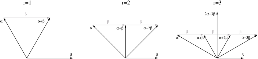
Figure 1: Short-root strings through a long root, for length² ratios $r=1,2,3$

For the long/short pairs in $B_{n}$, $C_{n}$ and $F_{4}$ ($r{=}2$) the role of (6.2)=0 is then taken by a four-root identity based on the quadruple $(\alpha,\beta,\alpha{+}\beta,\alpha{+}2\beta)$. With scalar products

$\cdot$	$\ \beta$	$\alpha{+}\beta$	$\ \alpha$	$\alpha{+}2\beta$
$\beta$	1	0	-1	1
$\alpha{+}\beta$	0	1	1	1
$\alpha$	-1	1	2	0
$\alpha{+}2\beta$	1	1	0	2

and the relevant wedge products all equal modulo sign, the equal-length pairs drop out, and the quadruple yields just four long/short pairs for the sum in (5.12),

$$-\ \frac{f_{\alpha}\,f_{\beta}}{\alpha{\cdot}x\;\beta{\cdot}x}\ +\ \frac{f_{\alpha}\,f_{\alpha+\beta}}{\alpha{\cdot}x\;(\alpha{+}\beta){\cdot}x}\ +\ \frac{f_{\alpha+2\beta}\,f_{\beta}}{(\alpha{+}2\beta){\cdot}x\;\beta{\cdot}x}\ +\ \frac{f_{\alpha+2\beta}\,f_{\alpha+\beta}}{(\alpha{+}2\beta){\cdot}x\;(\alpha{+}\beta){\cdot}x}\ .$$ (6.5)

This expression vanishes only when it must, namely for

$$f_{\alpha}\ =\ f_{\alpha+2\beta}\ =:\ f_{\textrm{L}}\qquad\textrm{and}\qquad f_{\beta}\ =\ f_{\alpha+\beta}\ =:\ f_{\textrm{S}}\ .$$ (6.6)

Like in the $ADE$ case, each non-orthogonal pair of roots defines a unique plane, which carries either a triple or a quadruple. Hence, the sum in (5.12) again splits into sums over the pairs of a triple or a quadruple, which yield zero individually. Since each plane shares its roots with other planes and all are connected unless the system is decomposable, all long roots come with the same coefficient $f_{\textrm{L}}$, and all short roots with $f_{\textrm{S}}$. The normalization in (5.13) then reads

$$f_{\textrm{L}}\sum_{\alpha\in\Phi^{+}_{\textrm{L}}}\alpha\otimes\alpha\ +\ f_{\textrm{S}}\sum_{\alpha\in\Phi^{+}_{\textrm{S}}}\alpha\otimes\alpha\ =\ \mathbbm{1}\ ,$$ (6.7)

where $\Phi^{+}_{\textrm{L}}$ and $\Phi^{+}_{\textrm{S}}$ stand for the positive long and short roots, respectively. Using

$$\sum_{\alpha\in\Phi^{+}_{\textrm{L}}}\alpha\otimes\alpha\ =\ \frac{rh^{\vee}{-}h}{r{-}1}\,\mathbbm{1}\qquad\textrm{and}\qquad\sum_{\alpha\in\Phi^{+}_{\textrm{S}}}\alpha\otimes\alpha\ =\ \frac{h{-}h^{\vee}}{r{-}1}\,\mathbbm{1}\ ,$$ (6.8)

the solution to (6.7) is a one-parameter family,

$$f_{\textrm{L}} \ =\ {\textstyle\frac{1}{h^{\vee}}}+(h{-}h^{\vee})t\ \ =\ {\textstyle\frac{1}{h}}+(h{-}h^{\vee})t^{\prime}\ ,$$ (6.9)

$$f_{\textrm{S}} \ =\ {\textstyle\frac{1}{h^{\vee}}}+(h{-}rh^{\vee})t\ =\ r\,\bigl{\{}{\textstyle\frac{1}{h}}+({\textstyle\frac{h}{r}}{-}h^{\vee})t^{\prime}\bigr{\}}\ ,$$

with $t=t^{\prime}-\frac{1}{hh^{\vee}}\in\mathbb{R}$. Therefore, we arrive at a family of prepotentials

$$F\ =\ -{\textstyle\frac{1}{2}}f_{\textrm{L}}\sum_{\alpha\in\Phi^{+}_{\textrm{L}}}(\alpha{\cdot}x)^{2}\,\ln|\alpha{\cdot}x|\ -\ {\textstyle\frac{1}{2}}f_{\textrm{S}}\sum_{\alpha\in\Phi^{+}_{\textrm{S}}}(\alpha{\cdot}x)^{2}\,\ln|\alpha{\cdot}x|\ .$$ (6.10)

Incidentally, the formulae (6.9) and (6.10) hold for all root systems, including the $ADE$ ($r{=}1$) and $G_{2}$ ($r{=3}$) cases. The only $r{=}3$ example, $G_{2}$, is trivial since of rank two, but let us anyway also prove the assertion for this case. The six positive roots of $G_{2}$ contribute 3 short/short, 3 long/long and 6 long/short pairs to the sum in (5.12). As argued before, the contributions of the equal-length pairs vanish by virtue of (6.2)=0, provided $f_{\alpha}{=}f_{\textrm{S}}$ for the short roots and $f_{\alpha}{=}f_{\textrm{L}}$ for the long ones. The mixed pairs yield

$${\textstyle\frac{-1}{\alpha{\cdot}x\,\beta{\cdot}x}}+{\textstyle\frac{1}{\alpha{\cdot}x\,(\alpha{+}\beta){\cdot}x}}+{\textstyle\frac{1}{(\alpha{+}3\beta){\cdot}x\,\beta{\cdot}x}}+{\textstyle\frac{1}{(\alpha{+}3\beta){\cdot}x\,(\alpha{+}2\beta){\cdot}x}}+{\textstyle\frac{1}{(2\alpha{+}3\beta){\cdot}x\,(\alpha{+}\beta){\cdot}x}}+{\textstyle\frac{1}{(2\alpha{+}3\beta){\cdot}x\,(\alpha{+}2\beta){\cdot}x}}$$ (6.11)

for a long root $\alpha$ and a short root $\beta$, with $\alpha{\cdot}\beta=-1$, which as simple roots generate the $G_{2}$ system. It is quickly verified that the above expression indeed vanishes, which proves our claim. Hence, for all Lie-algebra root systems, we have proved the identity

$$\smash{\sum_{\alpha,\beta\atop(\alpha\neq\beta)}}\!\frac{\alpha{\cdot}\beta}{\alpha{\cdot}x\ \beta{\cdot}x}\ =\ 0\qquad\textrm{for}\qquad(\alpha,\beta)\ \in\ \bigl{(}\Phi^{+}_{\textrm{L}},\Phi^{+}_{\textrm{L}}\bigr{)}\ \textrm{or}\ \bigl{(}\Phi^{+}_{\textrm{S}},\Phi^{+}_{\textrm{S}}\bigr{)}\ \textrm{or}\ \bigl{(}\Phi^{+}_{\textrm{L}},\Phi^{+}_{\textrm{S}}\bigr{)}\ ,$$ (6.12)

which is effectively equivalent to the WDVV equation. Our solution (6.9) for the $f$ coefficients generalizes the one of [9, 10] and reduces to them at $t{=}0$. One might think that the one-parameter freedom is ficticious since $f_{\textrm{L}}$ and $f_{\textrm{S}}$ may be absorbed into the roots. However, this is not so because $f_{\textrm{L}}$ and $f_{\textrm{S}}$ may have opposite signs, which is crucial for constructing $U$ solutions in this $F$ background.

We have also checked the non-crystallographic Coxeter groups $H_{3}$, $H_{4}$ and $I_{2}(p)$ for $p{=}5$ and $p{>}6$. Of these, the dihedral $I_{2}$ series

$$\{\alpha\}\ =\ \{\ \cos(k\pi/p)\,e_{1}+\,\sin(k\pi/p)\,e_{2}\ |\ k=0,1,\ldots,p{-}1\ \}$$ (6.13)

trivially fulfils (5.10), as it is of rank two.

Figure 2: Root systems of the dihedral groups $I_{2}(p)$ for $p=2,3,4,5,6$

7 $U{=}0$ solutions: orthocentric simplices

In order to generalize the root-system solutions found in the previous section, in this section we take a more general look at the $n{=}3$ case. Again, the goal is to solve the WDVV equation (5.12) and the homogeneity condition (5.13) for $f_{R}{=}0$.

Previously we have mentioned that any set of $p{\geq}2$ covectors in $n{=}2$ dimensions solves (4.2), because the WDVV equation is empty and (5.7) only serves to restrict $f_{\alpha}$ and $f_{R}$. We now deliver a simple argument. Let us represent a covector $\alpha\in\mathbb{R}^{2}$ by a complex number $a\in\mathbb{C}$. Then, the traceless and the trace part of the homogeneity condition (5.7) translate to

$$\sum_{a}f_{a}\,a^{2}\ =\ 0\qquad\textrm{and}\qquad\sum_{a}f_{a}\,a\bar{a}\ =\ 2\,(1{-}f_{R})\ ,$$ (7.1)

respectively, where $\bar{a}$ is the complex conjugate of $a$ and $f_{a}\equiv f_{\alpha}\in\mathbb{R}$. Since the length of each covector can be changed by rescaling the corresponding $f$, it is evident that for more than one covector one can always select these coefficients in such a way that the complex numbers $f_{a}\,a^{2}$ form a closed polygonal chain in two dimensions, thus satisfying the first of (7.1). A common rescaling then takes care of the second equation as well, while $f_{R}$ can still be dialed at will. Therefore, by taking the complex square roots of the edge vectors of any closed polygonal chain, we obtain an admissible set of covectors.

Before moving on to three dimensions, it is instructive to work out the $f_{\alpha}$ coefficients from the homogeneity condition (5.13) for $f_{R}{=}0$ and $n{=}2$. For the case of two covectors $\{\alpha,\beta\}$, necessarily $\alpha{\cdot}\beta=0$. For $p{=}3$ coplanar covectors $\{\alpha,\beta,\gamma\}$, the homogeneity condition (5.13) uniquely fixes the $f$ coefficients to

$$f_{\alpha}\ =\ -\frac{\beta\cdot\gamma}{\alpha{\wedge}\beta\ \gamma{\wedge}\alpha}\qquad\textrm{and cyclic}\ ,$$ (7.2)

due to the identity

$$\beta{\wedge}\gamma\ \beta{\cdot}\gamma\ \alpha_{i}\alpha_{j}\ +\ \textrm{cyclic}\ =\ -\alpha{\wedge}\beta\ \beta{\wedge}\gamma\ \gamma{\wedge}\alpha\ \delta_{ij}\ .$$ (7.3)

The traceless part of the homogeneity condition should imply the single WDVV equation (5.12) in two dimensions. Indeed, the choice (7.2) turns the latter into

$$\alpha{\wedge}\beta\ \gamma{\cdot}x\ +\ \beta{\wedge}\gamma\ \alpha{\cdot}x\ +\ \gamma{\wedge}\alpha\ \beta{\cdot}x\ =\ 0$$ (7.4)

which is identically true. Without loss of generality we may assume that $\alpha+\beta+\gamma=0$, i.e. the three covectors form a triangle. In this case we have $\alpha{\wedge}\beta=\beta{\wedge}\gamma=\gamma{\wedge}\alpha=2A$, where the area $A$ of the triangle may still be scaled to ${\textstyle\frac{1}{2}}$, and (7.2) simplifies to

$$f_{\alpha}\ =\ -\frac{\beta\cdot\gamma}{4\,A^{2}}\qquad\textrm{and cyclic}\ .$$ (7.5)

Figure 3: Triangular configuration of covectors

In dimension $n{=}3$, the minimal set of three covectors must form an orthogonal basis, with $f_{\alpha}=1/\alpha{\cdot}\alpha$. Let us skip the cases of four and five covectors and go to the situation of $p{=}6$ covectors because the homogeneity condition (5.13) then precisely determines all $f$ coefficients. However, it is not true that six generic covectors can be scaled to form the edges of a polytope. The space of six rays in $\mathbb{R}^{3}$ modulo rigid SO(3) is nine dimensional, while the space of tetrahedral shapes (modulo size) has only five dimensions. In order to generalize the $n{=}2$ solution above, let us assume that our six covectors can be scaled to form a tetrahedron, with edges $\{\alpha,\beta,\gamma,\alpha^{\prime},\beta^{\prime},\gamma^{\prime}\}$ where $\alpha^{\prime}$ is dual to $\alpha$ and so on.

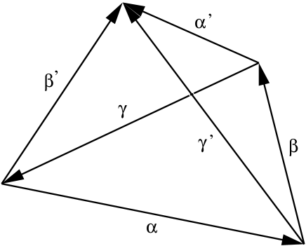
Figure 4: Tetrahedral configuration of covectors

Any such tetrahedron is determined by giving three nonplanar covectors, say $\{\alpha,\beta,\gamma^{\prime}\}$, which up to rigid rotation are fixed by six parameters, corresponding to the shape and size of the tetrahedron.

Let us try employing the triangle result (7.5) to patch together the unique solution to the homogeneity condition (5.13) for the tetrahedron. To satisfy the traceless part of the relation, we take the $f$ coefficients around any face to be proportional to the triangular ones (7.5). Now each edge is shared by two triangular faces, so we should have

$$f_{\alpha}\ =\ -\lambda_{\alpha\beta\gamma}\,\beta{\cdot}\gamma\ =\ -\lambda_{\alpha\beta^{\prime}\gamma^{\prime}}\,\beta^{\prime}{\cdot}\gamma^{\prime}$$ (7.6)

and so forth cyclicly around the triangles $\langle\alpha\beta\gamma\rangle$ and $\langle\alpha\beta^{\prime}\gamma^{\prime}\rangle$, with coefficients $\lambda_{\cdots}$ depending only on the triangle indicated. It is then tempting to put

$$f_{\alpha}\ =\ -\lambda\ \beta{\cdot}\gamma\ \beta^{\prime}{\cdot}\gamma^{\prime}\ ,\qquad f_{\beta}\ =\ -\lambda\ \gamma{\cdot}\alpha\ \gamma^{\prime}{\cdot}\alpha^{\prime}\ ,\qquad f_{\gamma}\ =\ -\lambda\ \alpha{\cdot}\beta\ \alpha^{\prime}{\cdot}\beta^{\prime}$$ (7.7)

and so on using the tetrahedral incidences, with $\lambda$ depending only on the volume $V$ of the tetrahedron. However, comparing the two previous sets of equations we see that this can only work if

$$\beta^{\prime}{\cdot}\gamma^{\prime}\ =\ \gamma^{\prime}{\cdot}\alpha^{\prime}\ =\ \alpha^{\prime}{\cdot}\beta^{\prime}\ =\ {\textstyle\frac{\lambda_{\alpha\beta\gamma}}{\lambda}}$$ (7.8)

and likewise for any three convergent edges dual to some face. These eight relations are non-generic but immediately equivalent to the three conditions

$$\alpha\cdot\alpha^{\prime}\ =\ 0\ ,\qquad\beta\cdot\beta^{\prime}\ =\ 0\ ,\qquad\gamma\cdot\gamma^{\prime}\ =\ 0$$ (7.9)

for the pairs of dual (skew) edges of the tetrahedron. Such tetrahedra, called ‘orthocentric’ [16], are characterized by the fact that all four altitudes are concurrent (in the orthocenter) and their feet are the orthocenters of the faces. The space of orthocentric tetrahedra is of codimension two inside the space of all tetrahedra and represents a three-parameter deformation of the $A_{3}$ root system (ignoring the overall scale).

For orthocentric tetrahedra, our ansatz (7.7) is successful: Due to the identity

$$\beta{\cdot}\gamma\ \beta^{\prime}{\cdot}\gamma^{\prime}\ \alpha_{i}\alpha_{j}\ +\ \beta{\cdot}\gamma^{\prime}\ \beta^{\prime}{\cdot}\gamma\ {\alpha^{\prime}}_{i}{\alpha^{\prime}}_{j}\ +\ \textrm{cyclic}\ =\ -36\,V^{2}\,\delta_{ij}\ ,$$ (7.10)

the homogeneity condition (5.13) is obeyed for

$$f_{\alpha}\ =\ -\frac{\beta{\cdot}\gamma\ \beta^{\prime}{\cdot}\gamma^{\prime}}{36\,V^{2}}\qquad\textrm{and}\qquad f_{\alpha^{\prime}}\ =\ -\frac{\beta{\cdot}\gamma^{\prime}\ \beta^{\prime}{\cdot}\gamma}{36\,V^{2}}$$ (7.11)

plus their cyclic images. What about the WDVV equation in this case? The 15 pairs of edges in the double sum of (5.12) group into four triples corresponding to the tetrahedron’s faces plus the three skew pairs. Using (7.11), the contribution of the $\langle\alpha\beta\gamma\rangle$ face becomes proportional to $\beta^{\prime}{\cdot}\gamma^{\prime}\,\gamma{\cdot}x+\textrm{cyclic}$, which vanishes thanks to (7.8). Repeating this argument for the other faces, we see that the concurrent edge pairs do not contribute to the double sum in (5.12), which leaves us with the three skew pairs. At this point, the orthocentricity again comes to the rescue via (7.9), and the WDVV equation is obeyed. Apparently, any reduction of the WDVV equation to some face already follows from the homogeneity condition, and the only independent projection is associated with the skew edge pairs.

Although we do not know the $f$ coefficients for a general tetrahedron, we can employ a dimensional reduction argument to prove that the WDVV equation already enforces the orthocentricity. Consider the limit $\hat{n}\cdot x\to\infty$ for some fixed covector $\hat{n}$ of unit length. Decomposing

$$\alpha\ =\ \alpha{\cdot}\hat{n}\;\hat{n}+\alpha_{\perp}\qquad\longrightarrow\qquad\alpha{\cdot}x\ =\ \alpha{\cdot}\hat{n}\;\hat{n}{\cdot}x+\alpha_{\perp}{\cdot}x$$ (7.12)

we see that any factor $\frac{1}{\alpha{\cdot}x}$ vanishes in this limit unless $\alpha{\cdot}\hat{n}=0$. Thus, only covectors perpendicular to $\hat{n}$ survive in (5.10), reducing the system to the hyperplane orthogonal to $\hat{n}$. In addition, $\frac{1}{R}\to 0$ as well, killing all radial terms in the process. In a general tetrahedron, take $\hat{n}$ to point in the direction of $\alpha{\wedge}\alpha^{\prime}$. Then, the limit $\hat{n}{\cdot}x\to\infty$ retains only the covectors $\alpha$ and $\alpha^{\prime}$, and the WDVV equation reduces to a single term, which vanishes only for $\alpha{\cdot}\alpha^{\prime}=0$. Equivalently, the plane spanned by $\alpha$ and $\alpha^{\prime}$ contains no further covector, and two covectors in two dimensions must be orthogonal. The same argument applies to $\beta{\cdot}\beta^{\prime}$ and $\gamma{\cdot}\gamma^{\prime}$, completing the proof.

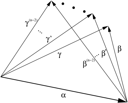
Figure 5: Faces sharing an edge of an $n$-simplex

This scheme may be taken to any dimension $n$. A simplicial configuration of ${\textstyle\frac{1}{2}}n(n{+}1)$ covectors is already determined by $n$ independent covectors, which modulo SO($n$) are given by ${\textstyle\frac{1}{2}}n(n{+}1)$ parameters. The homogeneity condition (5.13) uniquely fixes the $f$ coefficients. Employing an iterated dimensional reduction to any plane spanned by a skew pair of edges and realizing that no other edge lies in such a plane, we see that the WDVV equation always demands such an edge pair to be orthogonal. This condition renders the $n$-simplex orthocentric and reduces the number of degrees of freedom to $n{+}1$ (now including the overall scale given by the $n$-volume $V$). In this situation we can write down the unique solution to both the homogeneity condition and the WDVV equation,

$$f_{\alpha}\ =\ \frac{\beta{\cdot}\gamma\ \beta^{\prime}{\cdot}\gamma^{\prime}\ \beta^{\prime\prime}{\cdot}\gamma^{\prime\prime}\ \cdots\ \beta^{(n-2)}{\cdot}\gamma^{(n-2)}}{(n!\ V)^{2}}\ ,$$ (7.13)

where the edge $\alpha$ is shared by the $n{-}1$ faces $\langle\alpha\beta\gamma\rangle$, $\langle\alpha\beta^{\prime}\gamma^{\prime}\rangle$, $\ldots$, $\langle\alpha\beta^{(n-2)}\gamma^{(n-2)}\rangle$, and we have oriented all edges as pointing away from $\alpha$. This formula works because any sub-simplex, in particular any tetrahedral building block, is itself orthocentric. To summarize, the WDVV solutions for simplicial covector configurations in any dimension are exhausted by an $n$-parameter deformation of the $A_{n}$ root system. The $n$ moduli are relative angles and do not include the ${\textstyle\frac{1}{2}}n(n{+}1)$ trivial covector rescalings, which, apart from the common scale, destroy the tetrahedron. It has to be checked whether our deformation coincides with the $A_{n}$ deformation found in [11] in a different setting.

As a concrete example, the reader is invited to work out the details for the generic (scaled) orthocentric 4-simplex with vertices

$$A:(0,0,0,0)\qquad B:(1,0,0,0)\qquad C:(x,y,0,0)\qquad{}$$ (7.14)

$$D:(x,{\textstyle\frac{x(1-x)}{y}},z,0)\qquad E:(x,{\textstyle\frac{x(1-x)}{y}},{\textstyle\frac{x(1-x)(y^{2}-x(1-x))}{y^{2}\,z}},w)\quad.$$

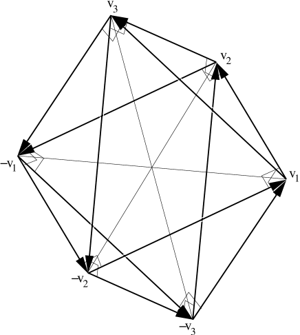
Figure 6: Octahedral configuration of covectors

Orthocentric simplices are not the only generalization of our analysis of six covectors in three dimensions. Recalling that $A_{3}=D_{3}$, we know that the six edges of a regular tetrahedron can be reassembled into one-half of a regular octahedron. Let us relax the regularity and look at a more general octahedron defined by six vertices $\pm v_{1}$, $\pm v_{2}$ and $\pm v_{3}$, which are fixed (up to rigid rotations) by six parameters, just like for the tetrahedron. For the full set of edges we need to include here also the negatives of all positive covectors,

$$\{\pm\alpha\}\ =\ \bigl{\{}\alpha_{(\pm i\pm j)}=\pm v_{i}{\pm}v_{j}\quad\textrm{for}\quad 1\leq i<j\leq 3\bigr{\}}\ .$$ (7.15)

With $f_{-\alpha}=f_{\alpha}$, the homogeneity condition uniquely fixes all $f$ coeficients. For the WDVV equation, let us again consider the dimensional reduction to the plane spanned by any pair of covectors, and restrict to the positive ones. Like for the tetrahedron, it turns out that such a plane contains either a triangular face or just two convergent covectors $\alpha_{(i+j)}$ and $\alpha_{(i-j)}$. The reduced WDVV equation requires a right angle between the latter, which puts $v_{i}{\cdot}v_{i}=v_{j}{\cdot}v_{j}$, and so all three vertices must have the same distance from the origin. We are not aware of a particular name for such octahedra, which admit a circumsphere. In any case, these two conditions and ignoring the overall scale reduce the modular space to a three-dimensional one, which we already identified as the space of orthocentric tetrahedral shapes.

The virtue of this alternative picture is a different generalization: In addition to the simplicial polytopes (related to $A_{n}$) we obtain as well hyperoctahedral polytopes (related to $D_{n}$) for WDVV solutions in any dimension, by letting $i{<}j$ in (7.15) run up to $n$. Such a configuration consists of $n(n{-}1)$ covectors plus their negatives, but is completely determined again by $n$ of these, for which ${\textstyle\frac{1}{2}}n(n{+}1)$ parameters are needed. Beyond $n{=}3$ the homogeneity condition (5.13) no longer fixes the $f$ coefficients. The WDVV equation now demands not only that $v_{i}{\cdot}v_{i}=v_{j}{\cdot}v_{j}$ but also that $\alpha_{(\pm i\pm j)}{\cdot}\alpha_{(\pm k\pm l)}=0$ for all indices mutually different. This is strong enough to enforce $v_{i}{\cdot}v_{j}\propto\delta_{ij}$, i.e. complete regularity for the hyperoctahedron. What remains for $n{>}3$ is just the $D_{n}$ root system (up to scale).

Our findings suggest that covector configurations corresponding to deformations of other roots systems may solve the WDVV equations as well. For verification, we propose to consider the polytopes associated with the weight systems of a given Lie algebra, since their edge sets are built from the root covectors. The idea is then to relax the angles of such polytopes and analyze the constraints from the homogeneity and WDVV equations. The $n$-dimensional hyper-tetrahedra and -octahedra we found emerge simply from the fundamental and vector representations of $A_{n}$ and $D_{n}$, respectively. Extending this strategy to other representations and Lie algebras could lead to many more solutions.

8 $U{\neq}0$ solutions: three-particle systems with $U_{\rm hom}{\equiv}0$

Let us finally try to turn on the other prepotential, $U{\neq}0$, in the background of the $F$ solutions already found. Unfortunately, we have no good strategy to solve (5.14) unless $U_{\rm hom}{\equiv}0$. Hence, in this section let us make the ansatz

$$U\ =\ -\sum_{\alpha}g_{\alpha}\,\ln|\alpha{\cdot}x|\ -\ g_{R}\,\ln R\ ,$$ (8.1)

and face the conditions (5.18) (for $n{>}2$) or (5.21) (for $n{=}2$). In the background of our irreducible root-system solutions, the Weyl group identifies the $f_{\alpha}$ and $g_{\alpha}$ coefficients for all roots of the same length. Hence, besides the $f_{\textrm{L}}$ and $f_{\textrm{S}}$ values in (6.9) we have couplings $g_{\textrm{L}}$ and $g_{\textrm{S}}$ for a number $p_{\textrm{L}}$ and $p_{\textrm{S}}$ of long and short positive roots, respectively. This simplifies the ‘sum rule’

$$\sum_{\alpha}f_{\alpha}\,\alpha{\otimes}\alpha\ =\ (1{-}f_{R})\,\mathbbm{1}\qquad{\buildrel\textrm{trace}\over{\longrightarrow}}\qquad\sum_{\alpha}\alpha{\cdot}\alpha\,f_{\alpha}\ =\ n\,(1{-}f_{R})$$ (8.2)

$$\textrm{to}\qquad 2f_{\textrm{L}}\,p_{\textrm{L}}\ +\ {\textstyle\frac{2}{r}}f_{\textrm{S}}\,p_{\textrm{S}}\ =\ n\,(1{-}f_{R})\qquad\buildrel g_{\textrm{L}},g_{\textrm{S}}\neq 0\over{\longrightarrow}\qquad p\ =\ n\,(1{-}f_{R})\ .$$ (8.3)

We first consider $n{>}2$, hence $g_{R}{=}0$ and $f_{R}{=}0$ for $C{\neq}0$. Since the total number $p$ of positive roots exceeds $n$ (except for $A_{1}^{\oplus n}$), we are forced to put either $g_{\textrm{S}}=0$ or $g_{\textrm{L}}=0$. This fixes all coefficients for $n{\geq}3$ to

either $$g_{\textrm{S}}=0\ ,\quad g_{\textrm{L}}=g\qquad\buildrel(\ref{UF2})(\ref{rootsumrule})\over{\longrightarrow}\qquad f_{\textrm{S}}={\textstyle\frac{r}{2}}{\textstyle\frac{n-p_{\textrm{L}}}{p_{\textrm{S}}}}\ ,\quad f_{\textrm{L}}={\textstyle\frac{1}{2}}$$ (8.4)

or $$g_{\textrm{S}}=g\ ,\quad g_{\textrm{L}}=0\qquad\buildrel(\ref{UF2})(\ref{rootsumrule})\over{\longrightarrow}\qquad f_{\textrm{S}}={\textstyle\frac{r}{2}}\ ,\quad f_{\textrm{L}}={\textstyle\frac{1}{2}}{\textstyle\frac{n-p_{\textrm{S}}}{p_{\textrm{L}}}}\ .$$ (8.5)

All simply-laced (ADEH) systems are immediately excluded because they have $f_{\alpha}={\textstyle\frac{1}{h^{\vee}}}$, as is seen in (6.4). In the non-simply-laced (BCFG) one-parameter family (6.9) with (6.10), however, there is always one member which obeys (8.4) or (8.5) and therefore (8.2). Furthermore, the trace of (5.18) follows from (6.12) because $g_{\alpha}$ and $f_{\beta}$ are constant on $\Phi^{+}_{\textrm{L}}$ and $\Phi^{+}_{\textrm{S}}$. The same consideration simplifies the expression (5.9) for the bosonic potential at $f_{R}{=}0{=}g_{R}$ to

$$V_{B}\ =\ \sum_{\alpha\in\Phi^{+}}\frac{v_{\alpha}}{(\alpha{\cdot}x)^{2}}\ ,\qquad\textrm{where}\qquad v_{\alpha}=\hbar^{2}{\textstyle\frac{f_{\alpha}^{2}}{r_{\alpha}^{3}}}\qquad\textrm{or}\qquad v_{\alpha}={\textstyle\frac{1}{r_{\alpha}}}(g_{\alpha}^{2}{+}{\textstyle\frac{\hbar^{2}}{4}})$$ (8.6)

for any positive root $\alpha$ with length${}^{2}=\frac{2}{r_{\alpha}}$, depending on whether $g_{\alpha}$ vanishes or not. It remains to check the traceless part of (5.18) for the choice (8.4) or (8.5). Unfortunately, this is never fulfilled for $n{>}2$, except in the reducible case of $A_{1}^{\oplus n}$. This failure extends to the deformed root systems, e.g. our orthocentric simplex backgrounds. This rules out $U_{\rm hom}{\equiv}0$ solutions to the flatness condition for all known irreducible WDVV backgrounds at $n{>}2$.

Therefore, in our search for $C{\neq}0$ solutions $(F,U)$ with $U_{\rm hom}{\equiv}0$, we are forced back to two dimensions, i.e. systems of not more than three particles. The plethora of $n{=}2$ WDVV solutions $F$ (parametrized by polygonal chains) may be cut down by invoking physical arguments. If a solution is supposed to describe the relative motion of three identical particles, then permuting their coordinates $x^{I}$ must be equivalent to permuting the covectors (up to sign). After separating the center-of-mass coordinate, the planar set $\{\pm\alpha\}$ should thus be invariant under the irreducible two-dimensional representation of ${\cal S}_{3}$. To visualize the situation, consider the $\mathbb{R}^{3}$ frame rotation by the orthogonal matrix

$$O\ =\ \begin{pmatrix}{\textstyle\frac{1}{\sqrt{2}}}&-{\textstyle\frac{1}{\sqrt{2}}}&0\\[6.0pt] {\textstyle\frac{1}{\sqrt{6}}}&\phantom{-}{\textstyle\frac{1}{\sqrt{6}}}&-{\textstyle\frac{2}{\sqrt{6}}}\\[6.0pt] {\textstyle\frac{1}{\sqrt{3}}}&\phantom{-}{\textstyle\frac{1}{\sqrt{3}}}&\phantom{-}{\textstyle\frac{1}{\sqrt{3}}}\end{pmatrix}\ :\qquad e_{I}\ \buildrel O\over{\longmapsto}\ \sqrt{\frac{2}{3}}\,\begin{pmatrix}\cos\phi_{I}\\[6.0pt] \sin\phi_{I}\\[6.0pt] {\textstyle\frac{1}{\sqrt{2}}}\end{pmatrix}\qquad\textrm{with}\quad\phi_{I}=\frac{2\pi I}{3}-\frac{\pi}{2}\ .$$ (8.7)

In the rotated frame, the 3-direction describes the center-of-mass motion, and the first two entries correspond to the relative-motion plane, on which the ${\cal S}_{3}$ representation acts by reflections and ${\textstyle\frac{2\pi}{3}}$ rotations. Reversely, the relative-motion plane is embedded back into the $\mathbb{R}^{3}$ configuration space of the total motion and rotated to the $x^{I}$ frame via

$$\alpha_{\text{rel}}\ =\ \biggl{(}\begin{matrix}\cos\phi\\[6.0pt] \sin\phi\end{matrix}\biggr{)}\quad\hookrightarrow\quad\alpha_{\text{tot}}\ =\ \Biggl{(}\begin{matrix}\cos\phi\\ \sin\phi\\ 0\end{matrix}\Biggr{)}\quad\buildrel O^{T}\over{\longmapsto}\quad\sqrt{\frac{2}{3}}\,\Biggl{(}\begin{matrix}\sin(\phi{+}\frac{\pi}{3})\\ \sin(\phi{-}\frac{\pi}{3})\\ -\sin\phi\end{matrix}\Biggr{)}\ =\ \Biggl{(}\begin{matrix}\alpha_{1}\\ \alpha_{2}\\ \alpha_{3}\end{matrix}\Biggr{)}\ ,$$ (8.8)

so that the new direction $(0,0,1)$ becomes the center-of-mass covector $\rho={\textstyle\frac{1}{\sqrt{3}}}(1,1,1)$. The ${\cal S}_{3}$ action is generated by $\phi\to\phi{+}{\textstyle\frac{2\pi}{3}}$ and $\phi\to\pi{-}\phi$, which produces all permutations of the $\alpha_{\text{tot}}$ entries and hence permutes the $\{x^{I}\}$ as required. The ${\cal S}_{3}$ orbit of $\alpha_{\text{rel}}$ is given by the angle set

$$\{\,\pm\phi\,,\,\pm\phi{+}{\textstyle\frac{2\pi}{3}}\,,\,\pm\phi{-}{\textstyle\frac{2\pi}{3}}\,\}\qquad{\buildrel\phi\ \textrm{special}\over{\longrightarrow}}\qquad\{\,0\,,\,\pm{\textstyle\frac{2\pi}{3}}\,\}\quad\textrm{or}\quad\{\,\pi\,,\,\pm{\textstyle\frac{\pi}{3}}\,\}\ ,$$ (8.9)

where the shorter orbits occur for $\phi=0$ or $\phi=\pi$, modulo ${\textstyle\frac{2\pi}{3}}$. The upshot is that the two-dimensional covectors must form a reflection-symmetric arrangement of $A_{2}$ systems!

In two dimensions, we take advantage of the radial terms in the structure equations and turn on all $g$ couplings, which yields (cf. (5.22))

$$f_{\alpha}={\textstyle\frac{1}{\alpha{\cdot}\alpha}}\ \forall\alpha\ ,\quad f_{R}=1{-}{\textstyle\frac{p}{2}}\ ,\quad g_{R}={\textstyle\frac{p-2}{p}}\,C\qquad\textrm{and}\qquad\!\sum_{\alpha<\beta}(g_{\alpha}{+}g_{\beta})\,\frac{\alpha{\cdot}\beta}{\alpha{\cdot}x\ \beta{\cdot}x}=0$$ (8.10)

for some ordering of covectors. The bosonic potential (5.9) specializes to

$$V_{B}\ =\ {\textstyle\frac{1}{2}}\sum_{\alpha}\bigl{(}g_{\alpha}^{2}+{\textstyle\frac{\hbar^{2}}{4}}\bigr{)}\frac{\alpha{\cdot}\alpha}{(\alpha{\cdot}x)^{2}}\ +\ {\textstyle\frac{p^{2}{-}4}{2}}\,\bigl{(}{\textstyle\frac{C^{2}}{p^{2}}}-{\textstyle\frac{\hbar^{2}}{4}}\bigr{)}\frac{1}{R^{2}}\qquad\textrm{with}\quad R^{2}=(x^{1})^{2}+(x^{2})^{2}\ .$$ (8.11)

This formula remains correct in the full three-dimensional configuration space, where one may add the center-of-mass contribution $V_{B}^{\text{com}}={\textstyle\frac{1}{2}}X^{-2}(C_{\text{com}}^{2}{+}{\textstyle\frac{\hbar^{2}}{4}})$. Please note, however, that $R$ still refers to the relative-motion subspace,

$$R^{2}\quad\hookrightarrow\quad x^{T}\Bigl{(}\begin{smallmatrix}1&0&0\\ 0&1&0\\ 0&0&0\end{smallmatrix}\Bigr{)}\,x\quad\buildrel O^{T}\over{\longmapsto}\quad{\textstyle\frac{1}{3}}\,x^{T}\Bigl{(}\begin{smallmatrix}\phantom{-}2&-1&-1\\ -1&\phantom{-}2&-1\\ -1&-1&\phantom{-}2\end{smallmatrix}\Bigr{)}\,x\ \neq\ {\textstyle\sum_{I}}(x^{I})^{2}\ .$$ (8.12)

Consider now for $\{\alpha\}$ a collection of $A_{2}$ systems, each with its own $g$ value and oriented at a particular angle in the relative-motion plane. Because each $A_{2}$ system fulfils the flatness condition by itself, we only have to compute the ‘cross terms’ in (8.10). Introducing the polar angles $\phi_{\alpha}$, $\phi_{\beta}$ and $\phi_{x}$ of $\alpha$, $\beta$ and $x$, respectively, the contributions

$$\frac{\alpha{\cdot}\beta}{\alpha{\cdot}x\ \beta{\cdot}x}\ =\ \frac{\cos(\phi_{\alpha}{-}\phi_{\beta})}{\cos(\phi_{x}{-}\phi_{\alpha})\;\cos(\phi_{x}{-}\phi_{\beta})}\ =\ \frac{\tan(\phi_{x}{-}\phi_{\alpha})-\tan(\phi_{x}{-}\phi_{\beta})}{\tan(\phi_{\beta}{-}\phi_{\alpha})}$$ (8.13)

to (8.10) collapse in telescopic sums, if and only if the reflection of any covector on any other one produces again a covector, and the couplings of mirror-image covectors are identified. Therefore, the orientations of the various $A_{2}$ systems must be isotropic, i.e. their collection forms an $I_{2}(p)$ system with $p=3q$. Ordering the positive roots according to their polar angles $\phi_{k}{=}k{\textstyle\frac{\pi}{p}}$ with $k=0,1,\ldots,p{-}1$, we get

$$g_{k}=g\quad\textrm{for $p$ odd}\qquad\textrm{or}\qquad g_{2\ell}=g\quad\textrm{and}\quad g_{2\ell+1}=g^{\prime}\quad\textrm{for $p$ even}\ ,$$ (8.14)

so that $\sum_{\alpha}g_{\alpha}={\textstyle\frac{2}{p}}C=p\,g$ or ${\textstyle\frac{p}{2}}(g{+}g^{\prime})$, respectively. Via (8.8) we further obtain

$$\frac{\alpha{\cdot}x}{\sqrt{\alpha{\cdot}\alpha}}\quad\to\quad\sqrt{{\textstyle\frac{2}{3}}}\,\Bigl{(}\sin(k{\textstyle\frac{\pi}{p}}{+}{\textstyle\frac{\pi}{3}})\cdot x^{1}\ +\ \sin(k{\textstyle\frac{\pi}{p}}{-}{\textstyle\frac{\pi}{3}})\cdot x^{2}\ -\ \sin(k{\textstyle\frac{\pi}{p}})\cdot x^{3}\Bigr{)}\ .$$ (8.15)

To see a few simple examples, let us give explicit results for $p=3$, 6 and 12.

$A_{2}$ model.
The minimal model, $p{=}3$, has $f_{R}{=}{-}{\textstyle\frac{1}{2}}$ and $g_{R}{=}{\textstyle\frac{1}{3}}C$ and a single free coupling $g={\textstyle\frac{2}{9}}C$. The radial terms are essential. In $F$ and $U$ appear the coordinate combinations

$$\frac{\alpha{\cdot}x}{\sqrt{\alpha{\cdot}\alpha}}\ \in\ \Bigl{\{}{\textstyle\frac{1}{\sqrt{2}}}(x^{1}{-}x^{2})\,,\,{\textstyle\frac{1}{\sqrt{2}}}(x^{1}{-}x^{3})\,,\,{\textstyle\frac{1}{\sqrt{2}}}(x^{2}{-}x^{3})\Bigr{\}}\qquad\textrm{and}$$ (8.16)

$$R^{2}\ \equiv\ {\textstyle\frac{1}{3}}\,x^{T}\Bigl{(}\begin{smallmatrix}\phantom{-}2&-1&-1\\ -1&\phantom{-}2&-1\\ -1&-1&\phantom{-}2\end{smallmatrix}\Bigr{)}\,x\ =\ {\textstyle\frac{1}{3}}\,\bigl{(}(x^{1}{-}x^{2})^{2}+(x^{2}{-}x^{3})^{2}+(x^{3}{-}x^{1})^{2}\bigr{)}\ ,$$

so that the bosonic potential becomes

$$V_{B}\ =\ \bigl{(}g^{2}{+}{\textstyle\frac{\hbar^{2}}{4}}\bigr{)}\,\biggl{(}\frac{1}{(x^{1}{-}x^{2})^{2}}+\frac{1}{(x^{2}{-}x^{3})^{2}}+\frac{1}{(x^{3}{-}x^{1})^{2}}\biggr{)}\ +\ {\textstyle\frac{5}{8}}\,\bigl{(}9g^{2}{-}\hbar^{2}\bigr{)}\,\frac{1}{R^{2}}\ .$$ (8.17)

$G_{2}$ model.
At $p{=}6$, two $A_{2}$ systems (with couplings $g$ and $g^{\prime}$) are superposed with a relative angle of $\frac{\pi}{6}$. With $f_{R}{=}{-}2$ and $g_{R}{=}{\textstyle\frac{2}{3}}C$ one has $g{+}g^{\prime}={\textstyle\frac{1}{9}}C$. We read off the combinations

$$\frac{\alpha{\cdot}x}{\sqrt{\alpha{\cdot}\alpha}}\ \ \in \Bigl{\{}{\textstyle\frac{x^{1}{-}x^{2}}{\sqrt{2}}}\,,\,{\textstyle\frac{2x^{1}{-}x^{2}{-}x^{3}}{\sqrt{6}}}\,,\,{\textstyle\frac{x^{1}{-}x^{3}}{\sqrt{2}}}\,,\,{\textstyle\frac{x^{1}{+}x^{2}{-}2x^{3}}{\sqrt{6}}}\,,\,{\textstyle\frac{x^{2}{-}x^{3}}{\sqrt{2}}}\,,\,{\textstyle\frac{-x^{1}{+}2x^{2}{-}x^{3}}{\sqrt{6}}}\Bigr{\}}\qquad\textrm{and}$$ (8.18)

$$R^{2} \ =\ {\textstyle\frac{1}{3}}\,\bigl{(}(x^{1}{-}x^{2})^{2}+\textrm{cyclic}\bigr{)}\ =\ {\textstyle\frac{1}{9}}\,\bigl{(}(2x^{1}{-}x^{2}{-}x^{3})^{2}+\textrm{cyclic}\bigr{)}$$

and obtain

$$V_{B}\ =\ \frac{g^{2}{+}{\textstyle\frac{\hbar^{2}}{4}}}{(x^{1}{-}x^{2})^{2}}\ +\ \frac{3\,({g^{\prime}}^{2}{+}{\textstyle\frac{\hbar^{2}}{4}})}{(2x^{1}{-}x^{2}{-}x^{3})^{2}}\ +\ \textrm{cyclic}\ +\ \frac{36(g{+}g^{\prime})^{2}{-}4\hbar^{2}}{R^{2}}\ .$$ (8.19)

$I_{2}(12)$ model.
Integrable three-particle models based on $A_{2}$ and $G_{2}$ have been discussed in the literature before. Among the infinity of novel models, we take $p{=}12$, which yields $f_{R}{=}{-}5$ and $g_{R}{=}{\textstyle\frac{5}{6}}C$, thus $g{+}g^{\prime}={\textstyle\frac{1}{36}}C$. In addition to the positive roots of the $G_{2}$ model (now all ‘even’ with coupling $g$), we have six ‘odd’ roots (with coupling $g^{\prime}$),

$$\frac{\alpha{\cdot}x}{\sqrt{\alpha{\cdot}\alpha}}\bigg{|}_{\textrm{odd}}\in\ \Bigl{\{}{\textstyle\frac{\tau x^{1}{-}x^{2}{-}\bar{\tau}x^{3}}{\sqrt{3}}}\,,\,{\textstyle\frac{\tau x^{1}{-}\bar{\tau}x^{2}{-}x^{3}}{\sqrt{3}}}\,,\,{\textstyle\frac{x^{1}{+}\bar{\tau}x^{2}{-}\tau x^{3}}{\sqrt{3}}}\,,\,{\textstyle\frac{\bar{\tau}x^{1}{+}x^{2}{-}\tau x^{3}}{\sqrt{3}}}\,,\,{\textstyle\frac{-\bar{\tau}x^{1}{+}\tau x^{2}{-}x^{3}}{\sqrt{3}}}\,,\,{\textstyle\frac{-x^{1}{+}\tau x^{2}{-}\bar{\tau}x^{3}}{\sqrt{3}}}\Bigr{\}}$$ (8.20)

where $\tau={\textstyle\frac{1}{2}}(\sqrt{3}{+}1)$ and $\bar{\tau}={\textstyle\frac{1}{2}}(\sqrt{3}{-}1)$. The bosonic potential reads

$$V_{B} = \frac{g^{2}{+}{\textstyle\frac{\hbar^{2}}{4}}}{(x^{1}{-}x^{2})^{2}}\ +\ \frac{3\,(g^{2}{+}{\textstyle\frac{\hbar^{2}}{4}})}{(2x^{1}{-}x^{2}{-}x^{3})^{2}}\ +\ \frac{\frac{3}{2}\,({g^{\prime}}^{2}{+}{\textstyle\frac{\hbar^{2}}{4}})}{(\tau x^{1}{-}\bar{\tau}x^{2}{-}x^{3})^{2}}\ +\ \frac{\frac{3}{2}\,({g^{\prime}}^{2}{+}{\textstyle\frac{\hbar^{2}}{4}})}{(\tau x^{1}{-}x^{2}{-}\bar{\tau}x^{3})^{2}}\ +\ \textrm{cyclic}$$ (8.21)

$$\ +\ \frac{630(g{+}g^{\prime})^{2}{-}\frac{35}{2}\hbar^{2}}{R^{2}}\ .$$

As has been displayed in (8.16) and (8.18), for permutation symmetric models the radial coordinate $R$ may be expressed via any triple $\Gamma$ of roots related by ${\textstyle\frac{\pi}{3}}$ rotations,

$$\sum_{\alpha\in\Gamma}\frac{\alpha{\otimes}\alpha}{\alpha{\cdot}\alpha}\ =\ {\textstyle\frac{3}{2}}\,\mathbbm{1}\qquad\longrightarrow\qquad R^{2}\ =\ {\textstyle\frac{2}{3}}\sum_{\alpha\in\Gamma}\frac{(\alpha{\cdot}x)^{2}}{\alpha{\cdot}\alpha}\ ,$$ (8.22)

so that, for instance, the radial parts of the prepotentials (5.6) may be rewritten as

$$F_{R}\ =\ -{\textstyle\frac{1}{6}}f_{R}\,\Bigl{(}\sum_{\alpha\in\Gamma}\frac{(\alpha{\cdot}x)^{2}}{\alpha{\cdot}\alpha}\Bigr{)}\,\ln\Bigl{(}\sum_{\alpha\in\Gamma}\frac{(\alpha{\cdot}x)^{2}}{\alpha{\cdot}\alpha}\Bigr{)}\ ,\quad U_{R}\ =\ -{\textstyle\frac{1}{2}}g_{R}\,\ln\Bigl{(}\sum_{\alpha\in\Gamma}\frac{(\alpha{\cdot}x)^{2}}{\alpha{\cdot}\alpha}\Bigr{)}\ .$$ (8.23)

The appearance of sums of roots under the logarithm is new.

We further comment that the radial terms for $I_{2}(3q)$ models with $q$ even can be eliminated in two ways. First, choosing $g{+}g^{\prime}=0$ and the classical limit $\hbar\to 0$, one obtains a conventional model (with covector terms only), but at the expense of putting $C{=}0$. Second, taking $g^{\prime}=0$ we can relax the condition $\alpha{\cdot}\alpha f_{\alpha}{=}1$ for the odd roots and thus put $f_{R}{=}0{=}g_{R}$ in this case, which then yields $\alpha{\cdot}\alpha f_{\alpha}={\textstyle\frac{4-p}{p}}$ for the odd roots and fixes $g={\textstyle\frac{2}{p}}C$. The bosonic potential in this special situation becomes

$$V_{B}\ =\ {\textstyle\frac{1}{2}}\,\bigl{(}g^{2}+{\textstyle\frac{\hbar^{2}}{4}}\bigr{)}\sum_{\alpha\ \textrm{even}}\frac{\alpha{\cdot}\alpha}{(\alpha{\cdot}x)^{2}}\ +\ {\textstyle\frac{\hbar^{2}}{8}}\,{\textstyle\frac{(4{-}p)^{2}}{p^{2}}}\,\sum_{\alpha\ \textrm{odd}}\frac{\alpha{\cdot}\alpha}{(\alpha{\cdot}x)^{2}}\ ,$$ (8.24)

so in the classical limit only half of the roots remain. Please note that this result differs from any limit of the generic case (8.11). Of course, the role of even and odd roots may be interchanged. The results of [3] and [6] describe examples of this kind.

The other dihedral groups may also be used to construct three-particle models, which however lack the permutation symmetry. Again we give a couple of prominent examples:

$A_{1}{\oplus}A_{1}$ model.
This model is reducible from the outset. From $p{=}2$ it follows that $f_{R}{=}0{=}g_{R}$ so that $g{+}g^{\prime}=C$. The two orthogonal positive roots are mapped via (8.15) to

$$\frac{\alpha{\cdot}x}{\sqrt{\alpha{\cdot}\alpha}}\ \in\ \Bigl{\{}{\textstyle\frac{1}{\sqrt{2}}}(x^{1}{-}x^{2})\,,\,{\textstyle\frac{1}{\sqrt{6}}}(x^{1}{+}x^{2}{-}2x^{3})\Bigr{\}}\ ,$$ (8.25)

and one finds

$$V_{B}\ =\ \frac{g^{2}{+}{\textstyle\frac{\hbar^{2}}{4}}}{(x^{1}{-}x^{2})^{2}}\ +\ \frac{3\,({g^{\prime}}^{2}{+}{\textstyle\frac{\hbar^{2}}{4}})}{(x^{1}{+}x^{2}{-}2x^{3})^{2}}\ .$$ (8.26)

Adding the cyclic permutations, one seems to arrive at the $G_{2}$ model but cannot produce the (necessary) radial term in this manner.

$BC_{2}$ model.
The $p{=}4$ case features angles of ${\textstyle\frac{\pi}{4}}$. With $f_{R}{=}{-}1$, $g_{R}{=}{\textstyle\frac{1}{2}}C$ and $g{+}g^{\prime}={\textstyle\frac{1}{4}}C$, the one-forms

$$\frac{\alpha{\cdot}x}{\sqrt{\alpha{\cdot}\alpha}}\in\Bigl{\{}{\textstyle\frac{1}{\sqrt{2}}}(x^{1}{-}x^{2})\,,\,{\textstyle\frac{1}{\sqrt{3}}}(\tau x^{1}{-}\bar{\tau}x^{2}{-}x^{3})\,,\,{\textstyle\frac{1}{\sqrt{6}}}(x^{1}{+}x^{2}{-}2x^{3})\,,\,{\textstyle\frac{1}{\sqrt{3}}}(-\bar{\tau}x^{1}{+}\tau x^{2}{-}x^{3})\Bigr{\}}$$ (8.27)

enter in

$$V_{B}=\frac{g^{2}{+}{\textstyle\frac{\hbar^{2}}{4}}}{(x^{1}{-}x^{2})^{2}}+\frac{3\,(g^{2}{+}{\textstyle\frac{\hbar^{2}}{4}})}{(x^{1}{+}x^{2}{-}2x^{3})^{2}}+\frac{\frac{3}{2}\,({g^{\prime}}^{2}{+}{\textstyle\frac{\hbar^{2}}{4}})}{(\tau x^{1}{-}\bar{\tau}x^{2}{-}x^{3})^{2}}+\frac{\frac{3}{2}\,({g^{\prime}}^{2}{+}{\textstyle\frac{\hbar^{2}}{4}})}{({-}\bar{\tau}x^{1}{+}\tau x^{2}{-}x^{3})^{2}}+\frac{6(g{+}g^{\prime})^{2}{-}\frac{3}{2}\hbar^{2}}{R^{2}}\ .$$ (8.28)

Again, this looks like a truncation of the model with $p\to 3p$. Regarding the explicit form of the above expressions, those are unique only up to rotations around the center-of-mass axis $\rho={\textstyle\frac{1}{\sqrt{3}}}(1,1,\ldots,1)$. Our convention has been to take the first root as $e_{1}\in\mathbb{R}^{2}$, which maps to ${\textstyle\frac{1}{\sqrt{2}}}(e_{1}{-}e_{2})\in\mathbb{R}^{3}$ under $O^{T}$ in (8.8).

The given examples should suffice to illustrate the general pattern of dihedral $n{=}2$ solutions with $U_{\rm hom}{\equiv}0$: The root systems of odd or even order give rise to one- or two-parameter three-particle models, which are permutation invariant only when the order is a multiple of three. Except for the reducible case of $I_{2}(2)$, the radial contributions are needed; they may disappear only when one of the two couplings in the even case vanishes.

9 $U{\neq}0$ solutions: three-particle systems in full

Any solution $U$ (including the trivial $U{\equiv}0$ one) for a given $F$ background can be modified by adding to it a homogeneous function $U_{\rm{hom}}$ satisfying $x^{i}\partial_{i}U_{\rm{hom}}=0$ and (5.14) for $C{=}0$. As we have seen in the previous section, including this freedom is in fact mandatory for finding $n{>}2$ solutions in the first place. In the three-particle case ($n{=}2$), however, we have identified an infinite series of special solutions, for which we now investigate the corresponding extension by $U_{\rm{hom}}$. In effect, this will add one additional coupling parameter to the models of the previous section.

To construct $U_{\rm{hom}}$ for a rank-two system specified by $\{\alpha,f_{\alpha},f_{R}\}$, it suffices to solve (5.15) for $C{=}0$, so that $f_{R}$ drops out. As $U_{\rm{hom}}$ depends only on the ratio $x^{2}/x^{1}$ we change to polar angles $\phi$ and $\phi_{\alpha}$ via

$${\textstyle\frac{x^{2}}{x^{1}}}\ =\ \tan\phi\qquad\textrm{and}\qquad{\textstyle\frac{\alpha\cdot x}{\sqrt{\alpha\cdot\alpha}}}\ =\ R\,\cos(\phi{-}\phi_{\alpha})$$ (9.1)

and arrive at

$$U_{\rm{hom}}^{\prime\prime}(\phi)-h(\phi)\,U_{\rm{hom}}^{\prime}(\phi)\ =\ 0\qquad\textrm{with}\qquad h(\phi)\ =\ \sum_{\alpha}f_{\alpha}\,\alpha{\cdot}\alpha\,\tan(\phi{-}\phi_{\alpha})\ .$$ (9.2)

This is easily integrated (with an integration constant $\lambda$) to

$$U_{\rm{hom}}^{\prime}(\phi)\ =\ \lambda\,\prod_{\alpha}\bigl{[}\cos(\phi{-}\phi_{\alpha})\bigr{]}^{-f_{\alpha}\,\alpha{\cdot}\alpha}\ \propto\ R^{2(1-f_{R})}\,\prod_{\alpha}(\alpha{\cdot}x)^{-f_{\alpha}\,\alpha{\cdot}\alpha}$$ (9.3)

and blows up on the lines orthogonal to the covectors $\alpha$. Generically, the singularities are $\sim(\alpha{\cdot}x)^{-1}$. Only in case some $g_{\alpha}$ vanishes, the corresponding $f_{\alpha}\alpha{\cdot}\alpha$ need not equate to one, thus $U_{\rm{hom}}^{\prime}$ may have a more general singularity structure. For a dihedral configuration with nonvanishing couplings $g_{\alpha}$ we can go further since $\phi_{\alpha}=k{\textstyle\frac{\pi}{p}}$ with $k=0,\ldots,p{-}1$, which yields

$$h(\phi)=\begin{cases}\!\phantom{-}p\,\tan(p\phi)&\textrm{for $p$ odd}\\[4.0pt] \!-p\,\cot(p\phi)&\textrm{for $p$ even}\end{cases}\Biggr{\}}\qquad\longrightarrow\qquad U_{\rm{hom}}^{\prime}=\begin{cases}\lambda\,\bigl{[}\cos(p\phi)\bigr{]}^{-1}&\textrm{for $p$ odd}\\[4.0pt] \lambda\,\bigl{[}\sin(p\phi)\bigr{]}^{-1}&\textrm{for $p$ even}\end{cases}\Biggr{\}}$$ (9.4)

and thus (‘$\simeq$’ means ‘modulo constant terms’)

$$U_{\rm{hom}}(\phi)\ \simeq\ {\textstyle\frac{1}{p}}\lambda\,\ln|\tan({\textstyle\frac{p}{2}}\phi{+}\delta)|\qquad\textrm{with}\qquad\delta\ =\ \Bigl{\{}\begin{matrix}{\textstyle\frac{\pi}{4}}&\textrm{for $p$ odd}\\ 0&\textrm{for $p$ even}\end{matrix}\ .$$ (9.5)

This may be compared with the particular solution (8.1),

$$U_{\rm{part}}\ =\ -\sum_{\alpha}g_{\alpha}\,\ln|\alpha{\cdot}x|-g_{R}\,\ln R\ \simeq\ -\sum_{\alpha}g_{\alpha}\,\ln|\cos(\phi{-}\phi_{\alpha})|-C\,\ln R\ ,$$ (9.6)

which, in the dihedral case, can be simplified to (remember that $\sum_{\alpha}g_{\alpha}{+}g_{R}=C$)

$$U_{\rm{part}}\ \simeq\ -C\,\ln R\ -\ \begin{cases}g\,\ln|\cos(p\phi)|&\textrm{for $p$ odd}\\[4.0pt] g\,\ln|\cos({\textstyle\frac{p}{2}}\phi)|+g^{\prime}\ln|\sin({\textstyle\frac{p}{2}}\phi)|&\textrm{for $p$ even}\ .\end{cases}$$ (9.7)

Combining $U_{\rm{part}}+U_{\rm{hom}}=U$ and lifting to the full configuration space $\mathbb{R}^{3}\ni(x^{I})$, we find

$$\partial_{I}U\ =\ -\sum_{\alpha}g_{\alpha}\,\frac{\alpha_{i}}{\alpha{\cdot}x}\ -\ {\textstyle\frac{p-2}{p}}C\frac{x_{i}}{R}\ +\ \lambda\,\biggl{(}\begin{smallmatrix}x^{2}{-}x^{3}\\ x^{3}{-}x^{1}\\ x^{1}{-}x^{2}\end{smallmatrix}\biggr{)}\,R^{p-2}\,\prod_{\alpha}(\alpha{\cdot}x)^{-1}\ .$$ (9.8)

For the simplest dihedral example, the $A_{2}$ system, with ($x^{ij}:=x^{i}{-}x^{j}$)

$$F\ =\ -{\textstyle\frac{1}{4}}\bigl{[}(x^{12})^{2}\ln|x^{12}|+(x^{23})^{2}\ln|x^{23}|+(x^{31})^{2}\ln|x^{31}|\bigr{]}\ +\ {\textstyle\frac{1}{4}}\,R^{2}\ln R\ ,$$ (9.9)

one gets

$$\partial_{I}U\ =\ [x^{12}x^{23}x^{31}]^{-1}\,\biggl{(}\begin{smallmatrix}[\lambda R-g(x^{31}{-}x^{12})]\,x^{23}\\ [\lambda R-g(x^{12}{-}x^{23})]\,x^{31}\\ [\lambda R-g(x^{23}{-}x^{31})]\,x^{12}\end{smallmatrix}\biggr{)}\ -\ {\textstyle\frac{3}{2}}g\,R^{-2}\,\biggl{(}\begin{smallmatrix}x^{1}\\ x^{2}\\ x^{3}\end{smallmatrix}\biggr{)}\ ,$$ (9.10)

which extends the bosonic potential (8.17) to

$$V_{B}\ = \bigl{(}g^{2}{+}{\textstyle\frac{2}{3}}\lambda^{2}{+}{\textstyle\frac{\hbar^{2}}{4}}\bigr{)}\,\biggl{(}\frac{1}{(x^{12})^{2}}+\frac{1}{(x^{23})^{2}}+\frac{1}{(x^{31})^{2}}\biggr{)}$$ (9.11)

$$+\ {\textstyle\frac{5}{8}}\,\bigl{(}9g^{2}{-}\hbar^{2}\bigr{)}\,\frac{1}{R^{2}}\ +\ \lambda\,g\,R\,\frac{(x^{12}{-}x^{23})(x^{23}{-}x^{31})(x^{31}{-}x^{12})}{(x^{12}x^{23}x^{31})^{2}}\ .$$

10 Conclusion

In this paper we systematically constructed conformal $(n{+}1)$-particle quantum mechanics in one space dimension with ${\cal N}{=}4$ supersymmetry, i.e. $su(1,1|2)$ invariance, and a central charge $C$. To begin with, the closure of the superalgebra produced a set of ‘structure equations’ (4.2) and (4.3) for two scalar prepotentials $U$ and $F$, which determine the potential schematically as $V={\textstyle\frac{1}{2}}U^{\prime}U^{\prime}+{\textstyle\frac{\hbar^{2}}{8}}F^{\prime\prime\prime}F^{\prime\prime\prime}$ plus fermionic terms. The structure equations consist of homogeneity conditions depending on $C$, a (generalized) WDVV equation (for $F$ alone) and a ‘flatness condition’ (for $U$ in the $F$ background).

Separating the center-of-mass degree of freedom reduces the configuration space from $\mathbb{R}^{n+1}$ to $\mathbb{R}^{n}$ for the relative motion. The ansatz (5.6) for the many-body functions $U$ and $F$ turned the structure equations into a decomposition of the identity (5.7) and nonlinear algebraic relations (5.10) and (5.18), for a set $\{\alpha\}$ of covectors in $\mathbb{R}^{n}$ and real coupling coefficients $g_{\alpha}$ (for $U$) and $f_{\alpha}$ (for $F$). The homogeneous part of $U^{\prime}$ is governed by a linear differential equation (5.14) (with $C{=}0$) of Fuchsian type. The case of three particles is special, because the WDVV equation is empty and so anything goes for $F$, but the flatness condition for $U$ is still nontrivial.

To find the prepotential $F$ it suffices to solve the WDVV equation (5.10). It is known that the roots of any finite reflection group provide a solution [9, 10], each giving rise to an interacting quantum mechanics model with $U{\equiv}0$ and thus $C{=}0$. Besides rederiving this result in a new fashion, we were able to generalize it in two ways: First, the $A_{n}$ root system may be deformed to a system of edges for a general orthocentric $n$-simplex, yielding a nontrivial $n$-parameter family of WDVV solutions which might agree with one found in [11]. Second, the relative weights for the long and the short roots contributing to $F$ are undetermined even in sign, so that the $BCF$-type solutions form one-parameter families.

For a nonzero central charge, in any given $F$ background one must turn on the prepotential $U$ by solving (5.14). Within our ansatz (5.6), this requires finding a suitable homogeneous part $U_{\rm{hom}}$ – an unsolved task. Only if in appropriate coordinates the system decomposes into subsystems not larger than rank two, then $U_{\rm{hom}}$ is not needed but can easily be found. Thus for the special case of three particles, i.e. $n{=}2$, the situation is simpler: the flatness condition (5.20) then permits the novel ‘radial terms’ which provided the necessary flexibility in our ansatz (5.6). Again the covectors were forced into a root system, which as of rank two must be dihedral. We explicitly constructed the full prepotentials (including $U_{\rm{hom}}$) for the new infinite dihedral series and displayed several examples lifted back to the original configuration space $\mathbb{R}^{3}\ni(x^{1},x^{2},x^{3})$. When the dihedral group and the central charge are fixed, the model depends on one or two tunable coupling parameters depending on the group order $p$ being odd or even. Permutation symmetry requires $p$ to be a multiple of 3. The previously found models [3, 6] turned out to be either decomposable or peculiar special cases of our dihedral systems, for which the ‘radial terms’ could by omitted. To summarize, we have classified all one-dimensional ${\cal N}{=}4$ superconformal quantum three-particle models based on covectors.

It remains an open problem to construct any irreducible $U{\neq}0$ solutions with more than three particles and to find all $U{\equiv}0$ solutions, i.e. the complete moduli space of the WDVV equation. To complement recent progress in mathematics on this issue [17], we would like to propose another strategy towards this goal: take any simple Lie algebra, select one of its irreducible representations and form the convex hull of its weight system. The edges of this polytope reproduce the roots, with certain multiplicities. Now consider a deformation of this polytope. Generically, the degeneracy of the edge orientations will be lifted, but the deformed collection of covectors still satisfies the incidence relation of the polytope. We suggest to test the WDVV equation on such configurations, generalizing the method successful for the fundamental $A_{n}$ representation. We are confident that this is feasible and will lead to further beautiful mathematical structures.

Note added

After a first version of this work had appeared on the arXiv, several aspects discussed here have been developed further in the three related papers [18]–[20].