Slow decay of concentration variance due to no-slip walls in chaotic mixing

Abstract

Chaotic mixing in a closed vessel is studied experimentally and numerically in different 2-D flow configurations. For a purely hyperbolic phase space, it is well-known that concentration fluctuations converge to an eigenmode of the advection-diffusion operator and decay exponentially with time. We illustrate how the unstable manifold of hyperbolic periodic points dominates the resulting persistent pattern. We show for different physical viscous flows that, in the case of a fully chaotic Poincaré section, parabolic periodic points at the walls lead to slower (algebraic) decay. A persistent pattern, the backbone of which is the unstable manifold of parabolic points, can be observed. However, slow stretching at the wall forbids the rapid propagation of stretched filaments throughout the whole domain, and hence delays the formation of an eigenmode until it is no longer experimentally observable. Inspired by the baker’s map, we introduce a 1-D model with a parabolic point that gives a good account of the slow decay observed in experiments. We derive a universal decay law for such systems parametrized by the rate at which a particle approaches the no-slip wall.

I Introduction

Many industrial applications involve the mixing of viscous fluids. Fields as diverse as chemical engineering, the pharmaceutical and cosmetics industries, and food processing depend on the stirring of initially heterogeneous substances to obtain a product with a sufficient degree of homogeneity. Viscous, confined or fragile fluids are best mixed by non-turbulent flows, which tend to be less effective at mixing than their turbulent counterpart. However, some laminar flows exhibit chaotic advection, meaning that they have chaotic Lagrangian trajectories Aref (1984); Ottino (1989), allowing them to rival turbulent flows in their ability to mix. The framework of chaotic advection and dynamical systems provides a useful characterization of mixers that relies on the nature of the phase space, or the stretching statistics of Lagrangian trajectories. However, an essential issue for the mixing of a diffusive passive scalar is to predict the rate at which the scalar concentration is homogenized by a given stirring protocol.

Various approaches including an eigenmode analysis Pierrehumbert (1994); Fereday et al. (2002); Wonhas and Vassilicos (2002); Sukhatme and Pierrehumbert (2002); Pikovsky and Popovych (2003); Thiffeault and Childress (2003); Fereday and Haynes (2004); Thiffeault (2004); Liu and Haller (2004); Haynes and Vanneste (2005), a large-deviation description of the stretching distribution Antonsen et al. (1995); Antonsen and Ott (1996), and multifractal formalism Ott and Antonsen (1989); Antonsen and Ott (1991) have provided insights into the structure of the mixing pattern and its decay rate. Of particular importance in some of these studies is the idea that for time-periodic flows the spatial mixing pattern becomes persistent, in the sense that it repeats itself in time but with a decreasing overall amplitude of fluctuations. Time-persistent spatial patterns have been observed in numerical simulations Pierrehumbert (1994); Sukhatme and Pierrehumbert (2002); Fereday and Haynes (2004), as well as in dye homogenization experiments in cellular flows Rothstein et al. (1999); Jullien et al. (2000); Voth et al. (2003), and have been related to the slowest decaying eigenmode of the advection-diffusion operator. The term strange eigenmode, originally coined by Pierrehumbert Pierrehumbert (1994), is used to describe these patterns. The eigenmode amplitude decays exponentially with time at a rate determined by its associated eigenvalue, and an exponential decay of concentration variance has indeed been observed in various systems Pierrehumbert (1994); Rothstein et al. (1999); Jullien et al. (2000); Sukhatme and Pierrehumbert (2002); Voth et al. (2003); Thiffeault and Childress (2003); Fereday and Haynes (2004); Haynes and Vanneste (2005).

However, such results were obtained either in idealized systems Pierrehumbert (1994); Fereday et al. (2002); Wonhas and Vassilicos (2002); Sukhatme and Pierrehumbert (2002); Thiffeault and Childress (2003); Fereday and Haynes (2004); Gilbert (2006), or in cellular flows Rothstein et al. (1999); Jullien et al. (2000); Voth et al. (2003). It has been suggested Chertkov and Lebedev (2003); Lebedev and Turitsyn (2004); Schekochihin et al. (2004); Salman and Haynes (2007) that mixing might be slower in large-scale bounded flows, because of slow stretching dynamics in the vicinity of a no-slip wall. The specific form of the velocity field at a no-slip wall was first noticed and exploited by Chertkov and Lebedev Chertkov and Lebedev (2003). The authors calculated concentration statistics by ensemble averaging over different realizations of a flow in a bounded domain with random time-dependence. They obtained a transient algebraic decay of the scalar variance attributed to the influence of the wall, followed by an asymptotic exponential phase. Shortly thereafter, experiments of elastic turbulence in a microchannel Burghelea et al. (2004) showed an anomalous scaling of mixing dynamics with the Péclet number, which the authors related to the predictions of Chertkov and Lebedev Chertkov and Lebedev (2003). Detailed numerical simulations of scalar advection by a short-correlated flow in a bounded domain were recently performed by Salman and Haynes Salman and Haynes (2007), who characterized the scalar decay with a multi-stage scenario that includes a transient algebraic decay. All theoretical and numerical studies Chertkov and Lebedev (2003); Lebedev and Turitsyn (2004); Salman and Haynes (2007) assumed that, in bounded flows, scalar fluctuations are rapidly completely exhausted in the bulk because of efficient stretching therein, while scalar inhomogeneity subsists only in a decreasing pool at the boundary.

In a previous letter Gouillart et al. (2007), we have reported on the first experimental observation of “slow” algebraic mixing dynamics imposed by a no-slip wall in a deterministic 2-D chaotic advection protocol. In the present paper, we explore in more detail the successive stages of mixing of a passive scalar in experiments and simulations of Stokes flow. For several chaotic advection protocols, a blob of dye is released in a closed vessel and homogenized. In contrast with all studies mentioned above, we focus here on the influence of the wall on the concentration field far from the boundary, which we show is contaminated by the algebraic dynamics near the wall. Our approach is based on a Lagrangian description of stretched filaments slowly fed from the wall into the bulk. A simplified one-dimensional model — a generalization of the baker’s map — allows us to describe the various mechanisms at play and to reproduce the main features of the evolution of the concentration probability distribution.

The paper is organized as follows. In Section II we review the main ingredients of chaotic mixing. We discuss the successive stages of mixing and the associated length scales, which are then illustrated on the pedagogical example of the well-studied hyperbolic baker’s map. For this ideal system, we relate the structure of the strange eigenmode to the unstable manifold of the least-unstable periodic point. Section III is the core of the paper. We first report on homogenization experiments conducted with a figure-eight protocol already described in Gouillart et al. (2007), which we complement by numerical simulations of a viscous version of the blinking vortex flow Aref (1984), and a modified version of the baker’s map with a parabolic point at the wall. In all cases, we observe anomalously slow mixing, that is an algebraic — rather than exponential — decay of concentration variance. We argue that this behavior is generic for two-dimensional mixers where the chaotic region extends to fixed no-slip walls. In such systems, poorly stretched fluid escapes the wall at a slow rate (controlled by no-slip hydrodynamics) through the unstable manifold of parabolic points on the wall. These poorly-mixed blobs contaminate the whole mixing pattern, up to the core of the domain where stretching is larger. We show that the modified baker’s map describes the experiments qualitatively and allows an analytic derivation of the observed scalings for the concentration distribution. A discussion on very long times, general initial conditions and hydrodynamical optimization is finally presented in Section V.

II Homogenization mechanisms

II.1 Stages and length scales of mixing

In this section, we describe briefly how the concentration field of a passive scalar (e.g. dye) evolves from an initially segregated state towards homogeneity. For illustrative purposes, we will consider the example shown in Figure 1 of a blob of dye of initial scale $\ell_{\mathrm{blob}}$ smaller than the velocity field scale $\ell_{\mathrm{v}}$, which is of the same order as the domain size $L$. Very viscous fluids typically support only laminar flows. Such flows may still lead to complicated, that is chaotic, Lagrangian trajectories Aref (1984); Ottino (1989).

Three different stages of the mixing process are apparent in Figure 1. An initial blob (Fig. 1(a)) is deformed by the stirring velocity field. At early times, the concentration pattern evolves as finer scales are created, yet the variance (the spatially-integrated squared fluctuations from the mean) is almost unchanged as the spatial scales are still too large for diffusion to be efficient (first stage, Fig. 1(b)). After several stretching and folding events, the width of a filament of dye stretched at a typical rate $\lambda$ stabilizes at the so-called Batchelor length

$$w_{\mathrm{B}}\mathrel{\raisebox{0.29707pt}{:}\!\!=}\sqrt{\kappa/\lambda},$$ (1)

with $\kappa$ the diffusivity, where the effects of compression and diffusion balance. Obviously, in a realistic flow, stretching is not constant, but the width of a filament quickly adapts to the local stretching rate $\lambda(\mathbf{x})$. The length scale $w_{\mathrm{B}}$ is the smallest that can be observed inside the concentration pattern: an initial blob with a scale greater than $w_{\mathrm{B}}$ is stretched and folded into many filaments that are compressed up to the diffusive scale $w_{\mathrm{B}}$. During a second stage (Fig. 1(c)), after a strip has stabilized at the width $w_{\mathrm{B}}$, the amplitude of the concentration profile decreases according to the stretching experienced by the strip, to ensure conservation of dye Balkovsky and Fouxon (1999); Thiffeault (2008). Different gray levels correspond to different stretching histories along the elongated image of the initial blob. Finally, since filaments are stretched but also folded, they are eventually pressed against each other, and their diffusive boundaries interpenetrate (third stage, Fig. 1(d)). Ultimately, homogenization takes place inside a “box” of size $w_{\mathrm{B}}$ through the averaging of many strips that have experienced different stretching histories and have therefore different amplitudes Villermaux and Duplat (2003).

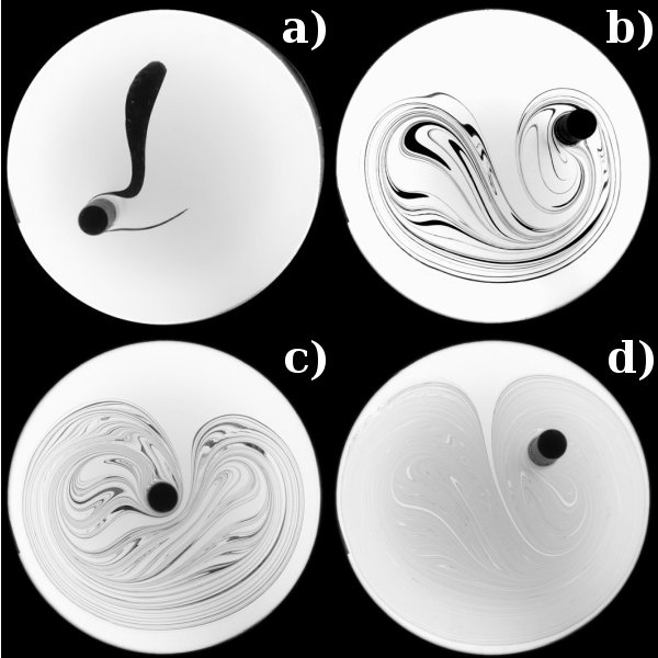
Figure 1: Successive stages of homogenization for a blob of dye stirred by the figure-eight protocol (see section III for details). (a) An initial blob is stretched by gradients in the velocity field. At early times, stretched filaments are still too broad for diffusion to be noticeable, and the concentration variance is constant. (b) As time increases, filaments are stretched and folded repeatedly, while a strip of white fluid coming from the boundary is inserted periodically at the core of the mixing pattern. As a result of this mass injection, the filamentary pattern grows slowly towards the boundary with time, while filaments become thin enough (c) for diffusion to become effective and cause the strips of dye to become more gray. Different gray levels correspond to different stretching histories. (d) Later, different filaments start interpenetrating, and the concentration field results from the averaging of concentration values coming from neighboring strips.

So far, the most satisfying explanation for the decay of inhomogeneity in chaotic mixing has been the strange eigenmode theory, initially proposed by Pierrehumbert in a 1994 paper Pierrehumbert (1994). The strange eigenmode is the second slowest decaying eigenmode of the advection-diffusion operator (the first trivial mode corresponds to a nondecaying uniform concentration). We consider in the following the case of periodic velocity fields, where the periodically-strobed strange eigenmode is an eigenvector of the time-independent Floquet operator. It decays at an exponential rate fixed by the real part of the corresponding eigenvalue. The projection of the initial concentration field on this eigenmode decays slower than the contributions from other eigenmodes, so that one expects the concentration field to converge rapidly to a permanent spatial pattern determined by the strange eigenmode, whose contrast decays exponentially.

A simple physical motivation for the strange eigenmode is as follows. The asymptotic concentration is governed by filaments that are pressed against each other in a box of width $w_{\mathrm{B}}$. But these filaments have explored the whole domain, and hence may possess different stretching histories Pierrehumbert (2000). The decay rate can thus depend on global properties of the flow Fereday and Haynes (2004); Haynes and Vanneste (2005). In particular, it is sensitive to spatial correlations, and cannot be expressed simply in terms of the stretching statistics.

Since the seminal paper of Pierrehumbert, strange eigenmodes have been observed in many numerical studies Fereday et al. (2002); Wonhas and Vassilicos (2002); Sukhatme and Pierrehumbert (2002); Pikovsky and Popovych (2003); Fereday and Haynes (2004). The proposed evidence for strange eigenmode were (i) the onset of permanent spatial concentration patterns and (ii) an exponential decay for the concentration variance, whose rate depended only weakly on the diffusion. Recurrent spatial patterns have also been observed in experiments where a viscous fluid is stirred by an array of magnets Rothstein et al. (1999); Jullien et al. (2000); Voth et al. (2003), yet the concentration decay seemed slower than exponential. In the following section, we briefly show how a strange eigenmode arises in a one-dimensional baker’s map, and relate the spatial structure of the eigenmode to the regions of lowest stretching.

II.2 Tracing out the strange eigenmode in a uniformly hyperbolic model

In this section, we describe how periodic points of a uniformly hyperbolic map affect the concentration field $C(x,t)$ of a low-diffusivity scalar, insofar as they determine the spatial structure of the observed strange eigenmode. We show that the concentration pattern obtained from an initial blob after successive iterations of the map is determined by the least unstable periodic point of the map, and its multifractal unstable manifold. For pedagogical reasons, we use one of the most-studied model of chaotic mixing, the inhomogeneous area-preserving baker’s map Farmer et al. (1983); Ott and Antonsen (1989); Antonsen and Ott (1991); Fereday et al. (2002).

The area-preserving baker’s map is defined on a two-dimensional square region by dividing the region in two strips, stretching, and re-stacking them. It has the property of mapping a $y$-independent distribution to another such distribution Fereday et al. (2002). We thus take our initial blob to be a strip uniform in the $y$-direction, and the baker’s map stretches and folds this strip to create more strips, leaving the concentration independent of $y$. We can thus focus on one-dimensional distributions that depend only on the $x$ coordinate: they represent a ‘cut’ across a striated pattern of strips like the pattern in Fig. 1. Hence, we limit ourselves to a one-dimensional version of the baker’s map which captures the essence of dynamics.

The baker’s map $f$ reads

$$f:x\mapsto f_{1}(x)\cup f_{2}(x)$$ (2a)

where

$$f_{1}(x)=\gamma x\,;\qquad f_{2}(x)=1-(1-\gamma)x$$ (2b)

and the union ($\cup$) symbol in (2a) means that $f$ is one-to-two: every point $x$ has two images given by $f_{1}(x)$ and $f_{2}(x)$. The parameter $\gamma$ satisfies $0<\gamma<1$ and controls the homogeneity of stretching, with $\gamma=1/2$ being the perfectly homogeneous case. The baker’s map is represented in Fig. 2.

Under the action of the baker’s map, the concentration profile evolves as

$$C(x,t+1)=C\bigl{(}f^{-1}(x),t\bigl{)}.$$ (3)

$f$ therefore transforms the concentration profile $C(x,t)$ at time $t$ into two images “compressed” by respective factors $\gamma$ and $1-\gamma$.

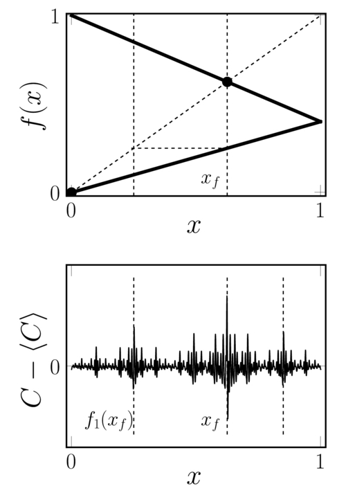
Figure 2: (a) One-dimensional baker’s map $f$, with two fixed points at $x=0$ and $x=1/(2-\gamma)$. For $\gamma<1/2$ the most stable fixed point is $x_{\mathrm{f}}=1/(2-\gamma)$. (b) Concentration profile obtained for an initial blob transformed by 17 iterations of $f$ ($\gamma=0.4,\,\kappa=10^{-5}$). Dominant “spikes” are located at $x_{\mathrm{f}}$ and (with decreasing amplitude) around its iterates (of decreasing stability).

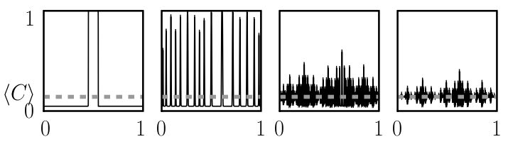
Figure 3: Main stages in the evolution of the concentration profile, from left to right. An initial blob is stretched into many filaments by the map. Once filaments reach the diffusive scale $w_{\mathrm{B}}$, intermediate concentration levels appear. The concentration profile takes the form of a persistent pattern — the strange eigenmode — when all boxes of size $w_{\mathrm{B}}$ contain an image of the initial unit interval.

First, we compute numerically the evolution of an initial blob under the action of $f$. The initial concentration

$$C(x,0)=C_{0}(x)=\begin{cases}1,\quad&x_{a}\leq x\leq x_{b};\\ 0,&\text{otherwise,}\end{cases}$$ (4)

is a strip of constant concentration between $x_{a}$ and $x_{b}$. Diffusion is mimicked by letting the concentration evolve diffusively during a unit time interval Pierrehumbert (2000); Fereday et al. (2002). During that interval, $C$ evolves according to the heat equation with diffusivity $\kappa$. We use periodic boundary conditions.

Figure 2 shows the concentration profile for a typical simulation with $\gamma=0.4$, after $17$ iterations of $f$ alternated with diffusive steps. We see that the system is well mixed, insofar as fluctuations of $C$ around its spatial mean $\langle C\rangle$ (which is conserved by the map) are very weak compared to the initial blob. Angle brackets denote a spatial average. A closer inspection reveals that fluctuations of $C$ have more important values at some points, so that the concentration pattern has distinctive spikes. Remarkably, the spatial pattern visible in Fig. 2(b) is permanent, as can be seen on the two rightmost profiles in Fig. 3: further iteration of the map does not change the form of $C$, only its amplitude. This shows that the concentration field converges very rapidly to an eigenfunction of the advection-diffusion operator, dubbed the strange eigenmode. We measure an exponential decay of the concentration variance, consistent with convergence to an eigenmode. Strange eigenmodes in the baker’s map, and their decay rate, have been studied in detail in Refs. Fereday et al. (2002); Wonhas and Vassilicos (2002); Gilbert (2006). Here we provide a simple and novel way to characterize the spatial structure of the strange eigenmode. More explicitly, we describe below how the strange eigenmode pattern traces out the unstable manifold of the periodic point of the map with weakest stretching. This echoes the description of invariant sets in open flows in terms of the chaotic saddle Tél et al. (2000).

As can be seen in Fig. 2, the map $f$ has two period-1 (fixed) points, one at $x=0$ and another at $x=x_{\mathrm{f}}\mathrel{\raisebox{0.29707pt}{:}\!\!=}1/(2-\gamma)$. Of course, since the 1-D baker’s map is one-to-two, both fixed points map to an additional point, so that the fixed points have iterates other than themselves. For $\gamma<1/2$ ($\gamma=0.4$ in Fig. 2), the second fixed point is less unstable than the first one, as the compression factor at $x_{\mathrm{f}}$ is smaller. We notice in Fig. 2 that the highest spike in the concentration pattern is located at $x=x_{\mathrm{f}}$, whereas spikes of decreasing height are located at iterates of $x_{\mathrm{f}}$: $f_{1}(x_{\mathrm{f}})$, $f_{2}(f_{1}(x_{\mathrm{f}})),\ldots$: the unstable manifold of $x_{\mathrm{f}}$ forms the backbone of the concentration pattern.

Let us examine more closely the iteration of the concentration pattern. After $t$ iterations of $f$, the initial blob has been transformed into $2^{t}$ strips compressed by factors $\gamma^{t},\,\gamma^{t-1}(1-\gamma),\dots,\,(1-\gamma)^{t}$. However, diffusion imposes that the width of an elementary strip saturates at the Batchelor width $w_{\mathrm{B}}$ where diffusion balances stretching. Using the range of possible stretchings in the map, we have

$$\sqrt{\frac{\kappa}{1-\gamma^{2}}}\leq w_{\mathrm{B}}\leq\sqrt{\frac{\kappa}{1-(1-\gamma)^{2}}},$$

where the diffusivity $\kappa$ has been rescaled by the size of the domain $L=1$ and the time-period $T=1$. We therefore approximate $w_{\mathrm{B}}\simeq\sqrt{\kappa/(1-\Gamma^{2})}$, where

$$\log\Gamma=\gamma\log(\gamma)+(1-\gamma)\log(1-\gamma)$$

is the Lyapunov exponent. The concentration profile of Fig. 2 has a typical variation scale of $w_{\mathrm{B}}$. Under repeated compression and diffusion steps, each elementary strip converges to a Gaussian peak of width $w_{\mathrm{B}}$ (see the second picture from left in Fig. 3), centered on iterates of the initial blob centroid $x_{c}\mathrel{\raisebox{0.29707pt}{:}\!\!=}(x_{a}+x_{b})/2$. The amplitude of each Gaussian strip is proportional to $\Lambda/w_{\mathrm{B}}$ to conserve total concentration, where $\Lambda$ is the multiplicative compression experienced by the strip.

The strange eigenmode regime is reached when the initial blob has been stretched enough so that its centroid has an iterate in every box of size $w_{\mathrm{B}}$ – that is, each box contains at least one image of the initial domain. In this regime, the concentration $C(x,t)$ measured at a point $x$ results from the addition of slightly shifted strips, whose centers are all iterates of $x_{c}$ that fit into a “box” of size $w_{\mathrm{B}}$ centered on $x$. The random averaging of such strips has been proposed as the mechanism controlling the homogenization rate Villermaux and Duplat (2003); Venaille and Sommeria (2007). However, due to strong time-correlations of stretching, this averaging is not a random uncorrelated process here. Fluctuations of $C(x)$ around $\langle C\rangle$ are typically inversely proportional to the number of iterates in the box centered on $x$ Villermaux and Duplat (2003). High spikes in the pattern therefore correspond to “boxes” with relatively few contributing iterates — i.e. images of the initial domain that have experienced relatively low compression.

Iterates of the initial profile located around $x_{\mathrm{f}}$ have experienced successive $1-\gamma$ factors during the last steps of the process while converging to the attracting periodic point $x_{\mathrm{f}}$, since they have been transformed by the second branch $f_{2}$ during all recent iterations. On average, these iterates have experienced compressions smaller than the mean compression $\Gamma^{t}$. This explains why the sharpest fluctuations are visible around $x_{\mathrm{f}}$, and with decreasing amplitude around iterates of $x_{\mathrm{f}}$ of decreasing stability. For example, all iterates around $f_{1}(x_{\mathrm{f}})$ have experienced a large number of successive $1-\gamma$ compressions, and an additional $\gamma$ compression during the latest iteration. In contrast, iterates around $x_{\mathrm{f}}$ have experienced only $(1-\gamma)$ compression steps in the last iterations, and fluctuations are greater.

We conclude that regions of low stretching control the structure of the concentration pattern. This behavior has already been illustrated for the case of mixed phase space (with elliptical islands or weakly connected chaotic domains) Pikovsky and Popovych (2003); Popovych et al. (2007), but also holds for purely hyperbolic domains with uneven stretching.

In addition, our description of the coherent structure of the strange eigenmode sheds a new light on why it is so difficult to predict the decay rate of the eigenmode Wonhas and Vassilicos (2002); Thiffeault and Childress (2003); Thiffeault (2004); Gilbert (2006). Fluctuations decrease at a rate determined by the subtle interplay of peaks corresponding to the successive iterates of $x_{\mathrm{f}}$, therefore spatial correlations of stretching histories play an important role in the decay rate, which cannot be related easily to the distribution of stretching in the map. We have provided here an example of concentration patterns dominated by the periodic structures with least stretching.

We now turn to the experimental study of mixing by fully chaotic flows in bounded domains. In such mixers, the dominant periodic structures are parabolic points on a no-slip boundary, and we show that such points impose slower algebraic dynamics.

III Parabolic points at the walls

In this section, we report on dye homogenization experiments conducted in a closed vessel where a single rod stirs fluid with a figure-eight motion. In this physical system, the phase portrait is not purely hyperbolic as it was in the baker’s map: we describe how separatrices (parabolic points) appear on the wall as a consequence of no-slip hydrodynamics. We show that these regions of low stretching slow down mixing and contaminate the whole mixing pattern up to its core, far from the wall. These experimental results were briefly presented in Gouillart et al. (2007). Here, results from a numerical simulation of a counter-rotating viscous blinking vortex protocol Aref (1984); Jana et al. (1994) are also presented. The dye pattern bears a strong resemblance to that of the figure-eight protocol, and we show that parabolic points at the walls are again responsible for algebraic decay. Inspired by the baker’s map studied in Sec. II.2, we introduce a simplified 1-D model that produces comparable algebraic mixing dynamics for this broad class of mixers.

III.1 Algebraic decay in experiments and numerical simulations

We first describe the essential features of the experimental set-up Gouillart et al. (2007). A cylindrical rod periodically driven on a figure-eight path gently stirs viscous sugar syrup inside a closed vessel of inner diameter $20~{}\text{cm}$ (Fig. 4(a)). The fluid viscosity $\nu=5\times 10^{-4}\,\text{m}^{2}\cdot\text{s}^{-1}$ together with rod diameter $\ell=16\,\text{mm}$ and stirring velocity $U=2~{}\text{cm}\cdot\text{s}^{-1}$ yield a Reynolds number $Re=U\ell/\nu\simeq 0.6$, consistent with a Stokes flow regime. A spot of low-diffusivity dye (Indian ink diluted in sugar syrup) is injected at the surface of the fluid (Fig. 1 (a)), and we follow the evolution of the dye concentration field during the mixing process (Fig. 1). The concentration field is measured through the transparent bottom of the vessel using a $12$-bit CCD camera at resolution $2000\times 2000$. This protocol is a good candidate for efficient mixing: we can observe on a Poincaré section (Fig. 4(b)) — computed numerically for the corresponding Stokes flow Finn and Cox (2001) — a large chaotic region spanning the entire domain, including the vicinity of the wall.

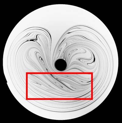
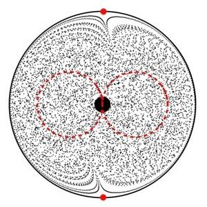
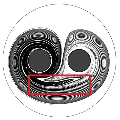
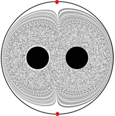
Figure 4: [Color online] Homogenization in closed flows for the experimental realization of the figure-eight protocol (a)–(b) and the numerical simulation of the contra-rotating blinking vortex (c)–(d). The heart-shaped mixing patterns are very similar: an upper cusp corresponds to a parabolic injection point on the boundary, while in the lower part of the pattern filaments are nicely packed in a parallel fashion. Although an annular unmixed region remains in the vicinity of the boundary, the partly-mixed pattern grows towards the boundary with time. This purely chaotic phase portrait is confirmed by the Poincaré section in (b) and (d), where a single trajectory fills the entire domain. In both cases two parabolic points can be inferred from the cusps in the upper and lower parts of the boundary. They correspond to separation points along whose unstable manifold fluid gets injected into the bulk, and to the corresponding reattachment at the opposite boundary. The frame in (a) and (d) indicates where measurements are taken.

We also perform numerical simulations of “dye homogenization” for a different stirring protocol. We consider a viscous version of the blinking vortex flow Aref (1984); Jana et al. (1994), that is, two counter-rotating vortices alternatively switched on and off. Following Jana et al. Jana et al. (1994), we study a realistic version of this protocol consisting of two large fixed rods placed on a diameter of a circular domain (see Fig. 4(c)). To mimic the blinking vortex, the two rods are rotated one after the other through angles $\theta$ and $-\theta$, in a counter-rotating fashion. This stirring protocol resembles the figure-eight, as the counter-rotating movement of the vortices draws fluid from the boundary in some part of the domain (the radial velocity $v_{\perp}$ is positive), whereas it is pushed towards the boundary in the other part ($v_{\perp}<0$). The flow parameters are $\theta=270^{\circ}$ (angular displacement of one rod at each half period), $r=0.7$ (distance between the rods), $r_{\mathrm{inner}}=0.2$ (radius of the rods). Length scale units are irrelevant here, and all distances are scaled by the radius of the cylindrical vessel $r_{\mathrm{outer}}=1$. In the same way, all times are rescaled by the stirring period $T$, so that we can work only with dimensionless quantities in the following. A Poincaré section shows (Fig. 4(d)) that the chaotic region spans the entire domain for this protocol as well. The evolution of a “blob of dye” is mimicked by computing the positions of $10^{6}$ particles — initialized inside a small square in the center of the domain — during 75 periods.

In the experiments, we measure the concentration field inside a large rectangle (see Fig. 4(a)) far from the wall. We plot the resulting variance and probability distributions functions (PDF) of the concentration in Fig. 5. We observe a decay of the concentration variance $\sigma^{2}(C)$ that is much closer to algebraic than exponential. (see Fig. 5(a)). In fact, as we will see in Sec. IV, the decay is well approximated by $\log\left(\tau_{\mathrm{W}}/t\right)/t^{2}$. This behavior persists until the end of the experiment (35 periods), by which time the variance has decayed by more than three orders of magnitude. We also note that PDFs of concentration have a wide shape, with power-law tails on both sides of the maximum (see Fig. 5(c)). Moreover, the PDFs of concentration are highly asymmetrical. A persistent white peak at zero-concentration values slowly transforms into a large shoulder at weak concentration values. This implies that the light-gray wing of the peak, corresponding to concentration values smaller than the most probable value, is more important than the dark-gray wing on the other side of the peak. Finally, the most probable value shifts slowly with time towards lower values.

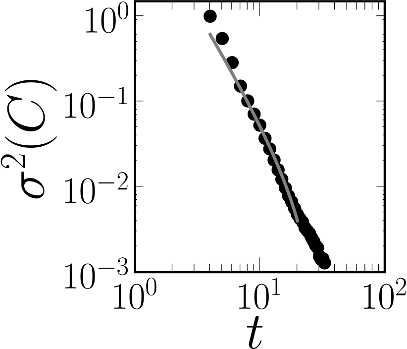
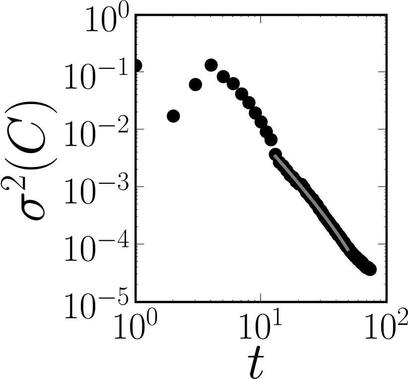
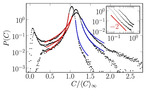
Figure 5: [Color online] Statistical properties of the concentration field measured in a central region (see frames in Fig. 4 (a) and (c)). The concentration variance (black circles) is consistent with the evolution law of Eq. (21) (gray solid line) – which is close to a power law – both in (a) the figure-eight protocol and (b) the blinking vortex. The decay of variance is much slower than an exponential, which would be the signature of a strange eigenmode. (c) Concentration PDFs after 13, 17 and 31 stirring periods in the figure-eight protocol. Both sides of the peak can be fitted by power laws $(C_{\mathrm{max}}-C)^{-2}$ (see solid line fits, and inset). Inset: left (light-gray) tail of the peak, $P(C)$ against $|C_{\mathrm{max}}(t)-C|$. Also note the persistence of a white peak at $C=0$, which transforms into large shoulder for longer times.

For the simulations, we compute a coarse-grained concentration field in a large area far from the boundary (rectangle in Fig. 4(c)). The coarse-graining (0.01 here) scale plays the role of the diffusive cut-off scale $w_{\mathrm{B}}$. Again, we observe an algebraic evolution of the concentration variance (shown in Fig. 5(b)) that is well fitted by the same decay law as in experiments.

III.2 Hydrodynamics near the wall

These experimental and numerical results are not consistent with the exponential evolution of a single eigenmode of the advection-diffusion operator. In order to understand these scalings, we first consider the various mechanisms at play. We will show that the observed slow mixing arises from a subtle combination of hydrodynamics, and the nature of the phase portrait at the wall.

As can be observed on the Poincaré section in Fig. 4(b), the chaotic region of the figure-eight protocol spans the whole domain, and no transport barriers are visible. (Elliptical islands can appear inside both loops of the figure-eight for a smaller rod, but for a large enough rod we did not detect such islands.) In particular, trajectories initialized close to the wall boundary also belong to the chaotic region. They eventually escape from this peripheral region to visit the remainder of the phase space, but only after a long time, as trajectories stick to the no-slip wall. This escape process takes place along the white cusp of the heart-shaped mixing region, as can be seen in Fig. 4. This white cusp is bisected by the unstable manifold of a separation point at the wall (upper red dot in Fig. 4 (b) and (d)). The manifold divides trajectories reinjected from the left and right of the separation point. Since stretching is very weak close to the wall, fluid drawn into the heart of the chaotic region from the wall is poorly mixed at the moment when it is injected, as opposed to fluid that has spent some time there already. Because we inject the initial blob of dye far from the boundary, poorly-stretched fluid injected from the boundary into the heart of the chaotic region consists of zero-concentration white strips that are interweaved into the mixing pattern (see Fig. 1 (b), (c) and (d)).

We can better characterize such white strips in terms of hydrodynamics near the no-slip wall. Consider the velocity field $\mathbf{v}$ near the vessel boundary. The wall can be treated as locally flat, and we define local coordinates $x_{\parallel}$ and $x_{\perp}$ that denote respectively the distance along and perpendicular to the wall. No-slip boundary conditions impose $v_{\parallel}=0$ for $x_{\perp}=0$ (on the wall) and the corresponding first-order linear scaling for small $x_{\perp}$,

$$v_{\parallel}=A(x_{\parallel})\,x_{\perp}+\mathrm{O}(x_{\perp}^{2}),\qquad\text{near the wall}.$$ (5)

Note that we are modeling the net velocity field, as evident in the Poincaré sections in Figs. 4(b) and 4(d), so we ignore the periodic time-dependence. Incompressibility implies

$$\frac{\partial v_{\parallel}}{\partial x_{\parallel}}+\frac{\partial v_{\perp}}{\partial x_{\perp}}=0,$$ (6)

which combined with (5) yields

$$v_{\perp}=-\tfrac{1}{2}A^{\prime}(x_{\parallel})\,x_{\perp}^{2}+\mathrm{O}(x_{\perp}^{3}).$$ (7)

Now from the Poincaré sections Figs. 4(b) and (d) we can see that the only trajectories that consistently approach the wall do so along a separatrix connected to the wall in the lower part of the vessel (the lower dot in each figure). All other trajectories recirculate into the bulk. The separatrix corresponds to a flow re-attachment point on the boundary Jana et al. (1994); Mezić (2001); Haller (2004), which we refer to as parabolic points. (All points on the boundary are parabolic fixed points, but the important ones for us have separatrices emanating from them. We only mean those distinguished points when we refer to parabolic fixed points.)

If we choose $x_{\parallel}=0$ to be the position of the lower separatrix, then the velocity on the separatrix is

$$v_{\parallel}\simeq 0,\qquad v_{\perp}\simeq-\tfrac{1}{2}a\,x_{\perp}^{2}\,,\qquad a\mathrel{\raisebox{0.29707pt}{:}\!\!=}A^{\prime}(0),$$ (8)

since $A(0)=0$ in order that the separatrix and the wall be on the same streamline. Note that the linear part of the flow around the re-attachment point vanishes, hence the name parabolic. The requirement that particles approach the wall along the separatrix implies $a>0$. Integrating $\dot{x}_{\perp}=v_{\perp}$ using Eq. (8), we find

$$x_{\perp}(t)=\frac{x_{0}}{1+atx_{0}},$$ (9)

where $x_{0}$ is the initial $x_{\perp}$ coordinate of the particle. Equation (9) predicts that the distance $d(t)$ between the wall and a particle on the lower separatrix shrinks as

$$d(t)\simeq{1}/{at},\qquad t\gg 1/ax_{0}.$$ (10)

This scaling was already derived in Chertkov and Lebedev (2003), from the same dimensional reasoning. The rate of approach along the separatrix constrains the approach to the wall of the entire mixing pattern. We verified both in the experiment and in the simulation that $d(t)$ is indeed well-approximated by a power-law scaling $d(t)\sim 1/t$. Note also that Eq. (10) implies that particles along the separatrix ‘forget’ their initial condition for long times. This can be seen in Figs. 4(a) and (c): material lines ‘bunch up’ against each other in the lower part of the domain faster than they approach the wall.

To ensure mass conservation, a quantity of unmixed white fluid scaling as ${\dot{d\mkern 8.0mu}\mkern-8.0mu}{}(t)\propto t^{-2}$ is injected periodically in the mixing pattern. As each newly injected white strip has approximately the same length (determined by the extent of the rod path), the width $\Delta(t)$ of a strip injected at time $t$ must also scale as

$$\Delta(t)\mathrel{\raisebox{0.29707pt}{:}\!\!=}\lvert{\dot{d\mkern 8.0mu}\mkern-8.0mu}{}(t)\rvert=1/at^{2},$$ (11)

where time $t$ has been rescaled by the period $T=1$.

The origin of our slow scaling now emerges. Clearly, the mixing pattern is chaotically stretched and folded by the rod at each half-cycle, in the same manner as in a baker’s map. Yet the folds are not stacked directly onto each other but are interweaved with the most recently injected white strip. Since each new white strip has a large width that decreases only algebraically with time, the decay of concentration is slowed down by this injection of unmixed material.

The dominant mechanism for mixing can be summed up as follows: (i) chaotic stretching imposes that the typical width of a filament of dye in the bulk (i.e. far from the wall) shrinks exponentially down to the diffusion or measurement scale; yet (ii) wide strips of unmixed fluid of width $\Delta(t)\propto t^{-2}$ are periodically interweaved with these fine structures. Both protocols have in common a chaotic region that spans the entire domain, which imposes the presence of parabolic separation points on the boundary Jana et al. (1994); Mezić (2001); Haller (2004). In the next section, we generalize the baker’s map model to include such a parabolic point at the boundary, and reproduce the dominant features observed experimentally and numerically.

III.3 A modified baker’s map model

We now wish to derive quantitative predictions to explain the observed algebraic scaling for the concentration variance. In the same spirit as in Section II.2, we simplify the two-dimensional problem by characterizing only one-dimensional concentration profiles $C(x,t)$ perpendicular to the stretching direction along which dye filaments align. The effect of the mixer during a half-period boils down to the action of a one-dimensional map that transforms concentration profiles by interweaving an unmixed strip of fluid with two compressed images of the profile. The width of each decays in time as $\Delta(t)\propto t^{-2}$, owing to the parabolic point on the boundary (Section III.1). We therefore mimic the behavior of our mixer with a one-dimensional map $g$, in the spirit of the baker’s map.

The map $g$ is defined on $[0,1]$ for simplicity. It evolves concentration profiles as in Eq. (3) and satisfies the following: (i) it is a continuous one-to-two function, to account for the stretching and folding process; (ii) the ‘wall’ at $x=0$ is a marginally unstable (i.e. parabolic) point of $g^{-1}$, so that the correct dynamics are reproduced by expanding $g^{-1}(x)\simeq x+ax^{2}+\cdots$ ($a>0$), for small $x$; (iii) because of mass conservation, at each $x$ the local slopes of the two branches, $g_{1}$ and $g_{2}$, of $g$ add up to $1$.

Other details of $g$ are unessential for our discussion. As in Section III.1, diffusion is mimicked by letting the concentration profile diffuse between successive iterations of the map (with no-flux boundary conditions). This model is a modified baker’s map, with a parabolic point at $x=0$, as opposed to the baker’s map in Section III.1, where the dynamics are purely hyperbolic. The expression of $g_{1}$ close to $x=0$ assures that the distance between the origin and successive iterates of a point by $g_{1}$ shrinks as $d(t)\simeq 1/at$, which is the same as Eq. (10) obtained in the experiments with no-slip hydrodynamics.

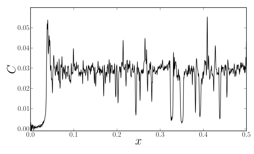
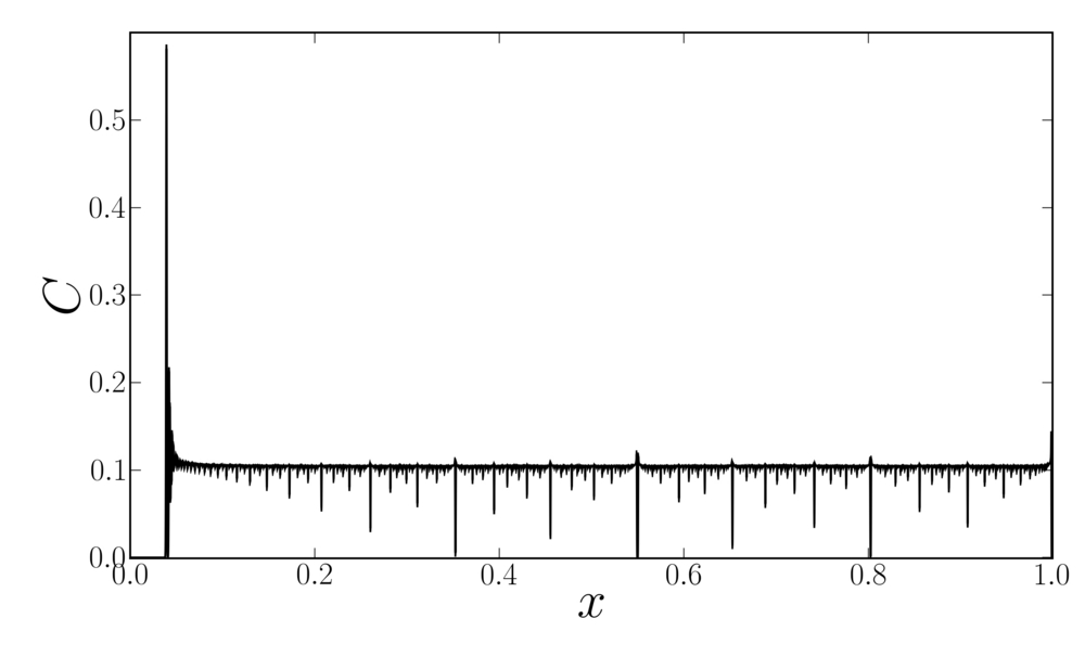
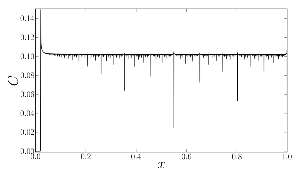
Figure 6: Concentration profiles from (a) the figure-eight experiment after 13 stirring periods, and from the 1-D model after (b) 25 and (c) 50 iterations of the map. Note the presence of “white fluid” ($C=0$) near $x=0$ in all cases.

We numerically evolve concentration profiles for the specific choice for $g$,

$$\left\{\begin{array}[]{cc}g_{1}(x)&=x-ax^{2}+(\gamma-1+a)x^{3},\\ g_{2}(x)&=1-ax^{2}+(\gamma-1+a)x^{3},\end{array}\right.$$ (12)

with $\gamma=0.55$ and $a=0.9$. We fix $\kappa=10^{-7}$. In our map $g_{1}(1)=g_{2}(1)=\gamma$, and as for the baker’s map we approximate by $\gamma$ the mean stretching realized by $g_{1}$, and by $(1-\gamma)$ the mean stretching realized by $g_{2}$ — although stretching is not constant along the two branches. We choose $\gamma\neq 0.5$ for an uneven stretching in the bulk, as in the experiments where fluid particles that stay close to the rod for long times experience more stretching than particles left behind. Our initial condition is of the form (4), with $x_{a}=(1-\delta)/2$ and $x_{b}=(1+\delta)/2$, i.e., a strip of width $\delta$ centered on $x_{c}=1/2$.

Figure 6 shows concentration profiles obtained after several iterations of the map. Strong similarities are observable between concentration profiles obtained in the experiment (Fig. 6(a)) and in the map (Fig. 6(b)–(c)). In both cases a thin layer of “white fluid” ($C=0$) is present near $x=0$. Its width decreases as $1/at$ due to the parabolic point on the boundary. In the experiment, the concentration pattern in the bulk (far from the wall) is characterized by sharp spikes at zero or low concentration values, whereas fluctuations are quite weak elsewhere. The sharp spikes correspond to white strips recently injected from the boundary into the bulk. For the map, the bulk pattern (far from $x=0$) is clearly dominated by a set of thin spikes, which are recently injected white strips. These white strips are images of the boundary region at $x=0$ by $g_{2}$, which are successively iterated by $g_{1}$ or $g_{2}$ after their injection in the bulk.

The suitability of our model is also strengthened by statistical properties of the concentration field, which closely resemble the experiment. Figure 7(a) shows the concentration variance for the map (measured in a central region) superimposed with experimental data: again we find an algebraic evolution. Moreover, there is a strong similarity between the concentration PDFs depicted in Fig. 7(b) and the experimental ones shown in Fig. 5(c). In particular, they both exhibit power-law tails. We will see in Section IV that our modified baker’s map is simple enough for the concentration statistics to be calculated explicitly.

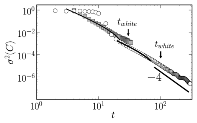
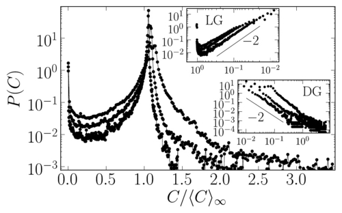
Figure 7: Variance and PDFs of the concentration field measured in a central region for a blob of dye transformed by the modified baker’s map (12). (a) The concentration variance (circles) shows an evolution close to a power-law, comparable to the figure-eight experiment (square symbols). The solid line fit and the $t^{-4}$ slope correspond respectively to the evolution dictated by Eqs. (21) and (28). (b) The concentration PDFs have wide power-law tails on both sides of the peak. The dark-gray tail corresponding to high concentration values decays much faster than the light-gray one (weak concentration values), since the latter is continuously fed by the injection of white fluid from the boundary.

IV Concentration statistics for the modified baker’s map

The simplicity of the model introduced in Section III.3 allows us to calculate the statistical properties of the concentration field. In this section, our interpretation is based mostly on our simplified model, although comparisons with the experiment are also made. We first consider the simple case of an initially-uniform blob, for which we characterize the concentration pattern by counting iterates of injected white strips, since these dominate the concentration pattern. We will treat more general initial conditions in Section V. We focus here on a central region where the concentration profile is at least partly mixed — that is, away from $x=0$, where $x$ is the map coordinate. The concentration PDFs and variance presented above have for example been measured in the range $x\in[0.2,0.9]$ in the map. We have checked that the variance measured in the whole domain evolves trivially as $1/t$, as it is dominated by the remaining white pool at the wall. (The variance in the numerical simulations of Salman and Haynes is measured in the whole domain and displays a $t^{-1}$ evolution during the algebraic phase Salman and Haynes (2007).) Here we are interested in the more complex evolution in the bulk, where stretching is high and the pattern seems “well mixed” after a few periods.

The modified baker’s map of Section III.3 transforms an initial blob of dye of width $s_{0}$ into an increasing number of strips with widths $s_{0}\Lambda_{1}\cdots\Lambda_{t}$, resulting from different stretching histories inside the mixed region, where $\Lambda_{t}$ is the compression experienced at time $t$. White strips also experience this multiplicative compression starting from their injection time. Because of diffusion, a strip of dye or white fluid is only compressed down to the local diffusive Batchelor scale $w_{\mathrm{B}}$, that we approximate by $w_{\mathrm{B}}=\sqrt{{\kappa}/{(1-\Gamma^{2})}}$, where

$$\log\Gamma=-\left\langle\log\left|\frac{\partial g^{-1}(x)}{\partial x}\right|\right\rangle$$ (13)

is the Lyapunov exponent and $\langle\cdots\rangle$ is the spatial mean taken over the region of measurement. For a moderate stretching inhomogeneity in the bulk, we expect $\Gamma$ to be close to $1/2$. In experiments as in simulations, we probe the concentration field on a pixel size, or box size, which is smaller than $w_{\mathrm{B}}$.

As in the baker’s map, different values of $C$ correspond to a different combination of superimposed strips in a box of size $w_{\mathrm{B}}$. We characterize $P(C)$ by considering the different widths of reinjected white strips that one can find in a such a box. We will distinguish between three generic cases corresponding to a partition of the histogram $P(C)$ in three different regions (see Fig. 5(c) and Fig. 7(b)): a white (W) peak at $C=0$ corresponding to recently-injected white strips that are still wider than $w_{\mathrm{B}}$, and light-gray (LG) and dark-gray (DG) tails corresponding to respectively smaller and larger concentrations than the peak (mean) concentration. Once we have quantified the proportion of boxes contributing to these different values of $C$, the variance is readily obtained as

$$\sigma^{2}(C)=\int(C-\langle C\rangle)^{2}P(C)\,{\mathrm{d}}C=\sigma^{2}_{\mathrm{W}}+\sigma^{2}_{\mathrm{LG}}+\sigma^{2}_{\mathrm{DG}}.$$ (14)

We treat each region of the histogram in turn in Sections IV.1–IV.3, and combine the results in Section IV.4.

IV.1 White pixels

Let us start with white (zero) concentration values that come from the stretched images of white strips injected before time $t$. White strips injected at an early time have been stretched and wiped out by diffusion, that is their width has become smaller than $w_{\mathrm{B}}$. A white strip injected at time $t_{0}$ has been compressed to a width $\Delta(t_{0})\Lambda_{t_{0}+1}\cdots\Lambda_{t}$ at time $t$. We neglect the spatial variation of $\Lambda(x)$ in the bulk and approximate $\Lambda_{t_{0}+1}\cdots\Lambda_{t}\simeq\Gamma^{t-t_{0}}$. The oldest white strips that can be observed have been injected at time $t=\tau_{\mathrm{i}}(t)$, where $\tau_{\mathrm{i}}(t)$ is defined by

$$\Delta(\tau_{\mathrm{i}})\,\Gamma^{t-\tau_{\mathrm{i}}}=w_{\mathrm{B}}\,.$$ (15)

Note that $t-\tau_{\mathrm{i}}(t)$ – that is the number of periods needed to compress an injected strip to $w_{\mathrm{B}}$ – is a decreasing function of time. After a time $t=\tau_{\mathrm{W}}$ defined by

$$\Delta(\tau_{\mathrm{W}})=w_{\mathrm{B}}\,,$$ (16)

the injected white strip is smaller than $w_{\mathrm{B}}$ and no white pixels can be observed. For $t<\tau_{\mathrm{W}}$, we can observe all white strips that are images of strips injected between $\tau_{\mathrm{i}}(t)$ and $t$, and the number of white pixels is proportional to

$$n_{\mathrm{W}}=\sum_{n=\tau_{\mathrm{i}}(t)+1}^{t}\Delta(n)=d(t)-d(\tau_{\mathrm{i}}(t)),$$ (17)

where $\Delta(t)=d(t)-d(t+1)$.

We now use the expression for $d(t)$ imposed by dynamics close to the parabolic point, $d(t)\simeq 1/at$, which yields for large $t$

$$n_{\mathrm{W}}\simeq(t-\tau_{\mathrm{i}})(a\tau_{\mathrm{i}}t)^{-1}.$$ (18)

From the definition (15) of the injection time $\tau_{\mathrm{i}}(t)$,

$$t-\tau_{\mathrm{i}}\simeq(\log{at^{2}}+\log{w_{\mathrm{B}}})/\log{\Gamma}$$ (19)

for large $t$, therefore

$$n_{\mathrm{W}}\simeq(\log{at^{2}}+\log{w_{\mathrm{B}}})/(at^{2}\log{\Gamma}).$$ (20)

The fraction of white pixels $n_{\mathrm{W}}$ is plotted versus time in Fig. 8(a). (There are no free parameters.) For later times, we find an excellent agreement between the data and the expression (20) for $n_{\mathrm{W}}$. Note that during the first few iterations $n_{\mathrm{W}}$ is constant: this corresponds to the initial phase when dye strips are still wider than $w_{\mathrm{B}}$ and diffusion is ineffective (i.e. up to $t$ such that $\delta\times\Gamma^{t}=w_{\mathrm{B}}$). The concentration variance is also almost constant during this initial phase, so we discard it. We deduce the contribution of the white pixels to the concentration variance for $t<\tau_{\mathrm{W}}$,

$$\sigma^{2}_{\mathrm{W}}=n_{\mathrm{W}}\langle C\rangle^{2}\simeq\delta^{2}\times\frac{\log{at^{2}}+\log{w_{\mathrm{B}}}}{at^{2}\log{\Gamma}}.$$ (21)

Of course, $\sigma^{2}_{\mathrm{W}}=0$ for $t>\tau_{\mathrm{W}}$, since by then there are no purely-white strips left.

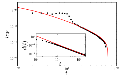
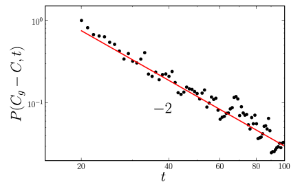
Figure 8: Simulations of dye homogenization by the modified baker’s map: (a) Fraction of white pixels (where $C=0$) $n_{\mathrm{W}}$ as a function of iterate (full circles). At early times diffusion has not yet started to broaden strips of dye, and $n_{\mathrm{W}}$ remains approximately constant. When $n_{\mathrm{W}}$ begins to decay, it closely follows Eq. (20) (solid line) obtained by counting the images of injected white strips that have not yet been compressed down to the diffusion scale $w_{\mathrm{B}}$. Inset: the distance between the dye pattern and the wall (measured by the position of the first peak in Fig. 6) evolves as $d(t)=1/at$ (solid line). (b) Probability of a light-gray concentration level with a given distance to the peak, i.e. probability that $\left|C_{\mathrm{g}}-\mathrm{d}C-C\right|\leq\epsilon$ ($C_{g}\sim 0.1$, $\mathrm{d}C=3\times 10^{-2}$, $\epsilon=10^{-3}$, as a function of time. $P(C_{\mathrm{g}}-C)$ agrees well with the $t^{-2}$ evolution predicted by Eq. (26) with $\Gamma\simeq 1/2$ (solid curve).

IV.2 Light-gray tail

We now focus on the distribution of light-gray values corresponding to white strips that have just been compressed below the cut-off scale $w_{\mathrm{B}}$. A white strip is first injected between images of the mixing pattern where fluctuations are lower (see Fig. 6). Fluctuations measured in a pixel are therefore mostly due to a recently-injected white strip that is superimposed onto a homogeneous distribution. We approximate the measured value $C$ as the average of the largest white strip with width $\ell_{\mathrm{W}}<w_{\mathrm{B}}$, and mixed “gray” fluid whose concentration is close to the most probable concentration $C_{\mathrm{g}}$. A box containing a white strip of scale $\ell_{\mathrm{W}}$ thus carries a concentration

$$C=C_{\mathrm{g}}\times(1-\ell_{\mathrm{W}}/w_{\mathrm{B}}),$$ (22)

and we can relate the concentration PDF $P(C)$ to the distribution $Q(\ell_{\mathrm{W}})$ of widths of images of the injected white strips in the following way:

$$P(C)=Q\big{(}\ell_{\mathrm{W}}\big{)}\left\lvert\frac{d\ell_{\mathrm{W}}}{dC}\right\rvert=\frac{w_{\mathrm{B}}}{C_{\mathrm{g}}}\,Q\big{(}\ell_{\mathrm{W}}\big{)}.$$ (23)

$Q(\ell_{\mathrm{W}})$ is easily retrieved from standard combinatorial arguments. A white strip injected at $t_{0}$ is transformed into $2^{t-t_{0}}$ images with scales $\Delta(t_{0})\Gamma^{t-t_{0}}$ (once again we consider only the mean stretching $\Gamma$, which amounts to matching a given concentration to a unique injection time). In a “quasi-static” approximation, we neglect the algebraic dependence of $\ell_{\mathrm{W}}$ (and hence of $C$ as well) on $t_{0}$ in the factor $\Delta(t_{0})$ compared to the exponential dependence in $\Gamma^{t-t_{0}}$. Therefore

$$Q(\ell_{\mathrm{W}})=(\ell_{\mathrm{W}}/\Delta(t_{0}))^{\log(2)/\log(\Gamma)}\times(1/\ell_{\mathrm{W}}\log{\Gamma}),$$ (24)

resulting in

$$P(C) =[\Delta(t)]^{\,\log{2}/\log{(\Gamma^{-1})}}\frac{w_{\mathrm{B}}}{C_{\mathrm{g}}(t)}\bigg{[}w_{\mathrm{B}}\left(1-\frac{C}{C_{\mathrm{g}}}\right)\bigg{]}^{\frac{\log{2}}{\log{\Gamma}}-1}$$

$$=\tilde{P}(t)\bigl{[}C_{\mathrm{g}}-C\bigr{]}^{(\log{2}/\log{\Gamma})-1}\;.$$ (25)

$P(C)$ thus has a power-law tail in the light-gray levels whose exponent depends on the mean stretching $\Gamma$. We observe satisfactory agreement between this prediction and both experimental data and numerical 1-D simulations (see Figs. 5(c) and 7(b)). Indeed, for the tail in Fig. 5(c) and Fig. 7(b) we measure $P(C)\propto(C-C_{\mathrm{g}})^{-\alpha}$ with $\alpha\lesssim 2$, consistent with $\Gamma\lesssim 1/2$, a fairly homogeneous stretching, as expected for $\gamma=0.55$. Also note that the amplitude of the light-gray tail decreases with time as a power law,

$$\tilde{P}(t)\propto[\Delta(t)]^{\,\log 2/\log(1/\Gamma)}\propto t^{-2(\log 2/\log(1/\Gamma))}.$$ (26)

We have plotted in Fig. 8(b) the probability of a concentration value at fixed distance from the maximum. The observed evolution scales as a power-law $t^{-2}$, as expected from our calculation. We deduce the contribution of light-gray pixels to the concentration variance,

$$\sigma^{2}_{\mathrm{LG}}=\tilde{P}(t)\int_{C_{\mathrm{min}}}^{C_{\mathrm{g}}}(C_{\mathrm{g}}-C)^{2-\alpha(\Gamma)}{\mathrm{d}}C\,,$$ (27)

where $\alpha(\Gamma)=1-\log{2}/\log{\Gamma}$, and $C_{\mathrm{min}}$ is the smallest concentration observed ($C_{\mathrm{min}}=0$ for $t<\tau_{\mathrm{W}}$ and $C_{\mathrm{min}}=C_{\mathrm{g}}(1-\Delta(t)/w_{\mathrm{B}})$ for $t>\tau_{\mathrm{W}}$). For $t<\tau_{\mathrm{W}}$ the integral is constant and $\sigma^{2}_{\mathrm{LG}}\propto\tilde{P}(t)\propto\Delta(t)\propto t^{-2}$. On the other hand, for $t\geq\tau_{\mathrm{W}}$,

$$\sigma^{2}_{\mathrm{LG}}=\frac{\tilde{P}(t)}{2+\alpha(\Gamma)}[C_{\mathrm{g}}-C_{\mathrm{min}}]^{\,3-\alpha(\Gamma)}\propto t^{-\left(6+2\frac{\log 2}{\log\Gamma}\right)}\,.$$ (28)

For $\alpha(\Gamma)\sim 2$ as we observed, the exponent in the above power law is about $-4$.

IV.3 Dark-gray tail

Let us now turn to the dark-gray part of the PDF. In our case, high concentration values correspond to black strips of dye that have experienced little compression, so that they have not been grayed-out by averaging with many other strips. This time, it is not sufficient to consider only the mean stretching $\Gamma$ to characterize such strips as we did in Sections IV.1 and IV.2, since stretching histories far from the mean are involved. Looking at the concentration profiles in Fig. 6, we observe that the highest concentration values come from the reinjection of black strips pushed to the pattern boundary where they have experienced lower stretching than inside the pattern core. Such a positive concentration fluctuation is then mixed with the remainder of the pattern as successive images are compressed by a factor of order $\Gamma$, in the same way as injected white strips. Many images of the initial blob may have aggregated inside a box of size $w_{\mathrm{B}}$. If the decay of this highest-concentration “cliff” is slower than $\Gamma^{t}$ — the decay of an injected fluctuation inside the bulk — we can apply the same method for computing the shape of the dark-gray tail as we did for white strips and the light-gray tail.

In the spirit of Eq. (22), we write

$$C=C_{\mathrm{g}}\times(1-\ell_{\mathrm{black}}/w_{\mathrm{B}})+\ell_{\mathrm{black}}/w_{\mathrm{B}},$$ (29)

and relate the width $\ell_{\mathrm{black}}$ to the injection time $t_{0}$ as in Section IV.2. This leads again to a power-law dependence $(C-C_{\mathrm{g}})^{-2}$, this time for the dark-gray tail. This is in good agreement with the observed scalings for both experimental and numerical PDFs (see Figs. 5(c) and 7(b)).

We now wish to estimate the time decay of the amplitude of this tail. To do so, we evaluate the amplitude of the highest concentration fluctuation, located on the left boundary of the pattern (see Fig. 6(b) and (c)). This will give us the concentration value for which a number of boxes of order 1 contribute to the histogram, and hence provide an approximation of the amplitude of the tail. The contribution of the dark-gray tail is tiny compared to the light-gray one, since, after a few periods, only a few boxes of size $w_{\mathrm{B}}$ on the border of the pattern have an amplitude significantly greater than the mean (see Figs. 6(b) and (c)), whereas the width of the remaining white pool is much larger. Moreover, we show below that this amplitude decays faster than the contribution of white strips.

We have plotted in Fig. 9 the decaying amplitude of the largest fluctuation in the pattern, that is of the leftmost box in the mixing pattern (Figs. 6(b) and (c)). The evolution during 200 periods reveals a first exponential decay, whose rate increases with the diffusivity, followed by a power-law phase with an exponent of about $-3$. A simple analysis explains this evolution. The amplitude of this fluctuation can be estimated as $\Lambda/w_{\mathrm{B}}$, where $\Lambda\simeq\prod_{i=1}^{t}g_{1}^{\prime}(g_{1}^{i}(1))$ is the compression factor experienced after $t$ periods at the boundary of the pattern (i.e. by the leftmost blob image). (This is true as long as the distance between the pattern and the wall is less than the diffusion scale at the boundary. We will discuss this final phase in Section V.1.) For early times dye strips do not yet feel the effect of the wall, and the stretching factor can be approximated by $\gamma^{t}$ (we use $\gamma$ instead of $\Gamma$ for evaluating the compression by repeated iterations of $g_{1}$), and we expect the decay to be exponential with a rate $\log\gamma$. This behavior is indeed observed for large enough diffusivities (Fig. 9(a)). For small diffusivities, few strips of dye are homogenized before the boundary of the mixing pattern reaches the wall region, where the effect of the parabolic point dominates, so we do not observe the first exponential phase.

For long times $g_{1}^{i}(1)\simeq(ai)^{-1}$, $g_{1}^{\prime}(g_{1}^{i}(1))\simeq 1-2/i$. The compression $\Lambda$ can be approximated by

$$\Lambda\simeq\gamma^{n_{0}}\prod_{i=n_{0}+1}^{t}(1-2/i).$$ (30)

The two factors in (30) account for (i) the exponential compression by successive factors of order $\gamma$ inside the bulk, and (ii) a weaker compression by factors converging slowly to $1$ as the boundary of the pattern approaches the wall and experiences a compression determined by the parabolic point at $x=0$ (Section III.2). The product $\prod_{i=n_{0}+1}^{t}(1-2/i)$ converges to a power law $t^{-2}$ for long times. The observed exponent is greater; this might come from a crossover between an exponential phase and the predicted $t^{-2}$ phase.

¿From the above analysis, we see that positive concentration fluctuations decay fast with time, compared to the contribution of the remaining white layer at $x=0$, which shrinks much more slowly. The contribution of the dark-gray tail to the concentration variance is very small compared to the light-gray tail, therefore we neglect it in the following computation of the variance.

It is important to note that the asymmetry of the concentration PDF persists because our mixer “remembers” the initial condition — a small black spot and a big white pool — even after very long times.

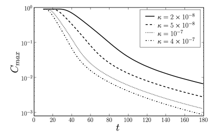
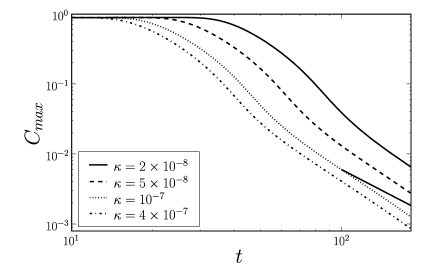
Figure 9: Amplitude $C_{\mathrm{max}}$ of the maximum positive concentration fluctuation, in log-linear (a) and log-log (b) coordinates, for different diffusivities. This corresponds to the amplitude of the leftmost spike of the concentration pattern, which has experienced weaker stretching than images of the initial blob in the core of the pattern. An exponential decay followed by a power-law evolution are evident. A line of slope $-2$ corresponding to the asymptotic evolution expected from Eq. (30) has been drawn for comparison.

In our experiments, additional contributions to the dark-gray tail come from dye particles trapped during some time in folds of the pattern where stretching is weak (notice the dark folds in Fig.1(a)). This 2-D effect is not present in our map. The dark-gray tail therefore consists of contributions from the border of the pattern, but also from these folds. Nevertheless, we have checked that this contribution is small compared to the light-gray tail, and decays rapidly with time.

IV.4 Total concentration variance

We finally sum all contributions from different parts of the PDF to obtain $\sigma^{2}(C)$, as in Eq. (14). From the above discussion, we distinguish two phases, $t<\tau_{\mathrm{W}}$ when the variance is dominated by the contribution of recently injected white strips that have not yet reached $w_{\mathrm{B}}$, and $t>\tau_{\mathrm{W}}$ when the most important fluctuations come from the mixing of white strips and gray fluid.

In the experiment, the crossover time $\tau_{\mathrm{W}}$ is estimated as $30$ periods. However, 3-D effects inside the fluid prevented us from conducting experiments for more than $35$ periods. For this early regime, fitting $\sigma^{2}(C)$ with $\sigma^{2}_{\mathrm{W}}\propto(2\log{t}+\log{w_{\mathrm{B}}})/t^{2}$ (gray line on Fig. 5(a)) gives good results, except close to $\tau_{\mathrm{W}}$ where the contribution of the light-gray tail starts to dominate. On the other hand, in numerical simulations we observe (Fig. 7(b)) both the $(2\log{t}+\log{w_{\mathrm{B}}})/t^{2}$ behavior (black line), which can be interpreted as in the experiment, and the $t^{-4}$ decay after $\tau_{\mathrm{W}}$ ($100$ periods for the case studied) given by $\sigma^{2}_{\mathrm{LG}}$. For long times, the observed power-law arises from the specific way of incorporating white strips whose width scales as $t^{-2}$ inside the mixing pattern.

Having established the origin of the scalings observed for the concentration variance and PDFs in our experiments, we turn in the next section to the analysis of asymptotically long times, different initial conditions, optimization, and offer some concluding remarks.

V Discussion

We have explained in the preceding sections the main features of our experiment. In this section we tie two loose ends: we examine the long-time behavior of the concentration in Section V.1, and look at the effect of initial conditions in Section V.2. Both aspects are more easily investigated in our simple map than in experiments, and our discussion is supported by numerical simulations of the 1-D map. In Section V.3 we address the issue of optimization of the mixing device based on what we learned about the role of walls. Finally, we close the paper with concluding remarks in Section V.4.

V.1 Recovering an eigenmode for long times

We now consider the asymptotic regime, when we can no longer approximate the injected variance by the contribution of a white strip of width $1/at^{2}$. This is because the mixing pattern is close enough to the wall that diffusion blurs the white layer at the boundary. For such large times, the mixing pattern can be described as an inverted half-Gaussian centered on $x=0$ (see Fig. 10(a)) that decays with time as fluid is reinjected in the bulk. At this time, fluctuations are very small in the rest of the pattern, and they are only controlled by the amplitude of the half-Gaussian. In this final regime, where the concentration pattern keeps a self-similar form with time, the concentration profile has eventually converged to an eigenmode of the advection-diffusion operator. The width of the half-Gaussian $w_{0}$ is determined by the point where stretching and diffusion balance,

$$w_{0}=\sqrt{\frac{\kappa}{1-g_{1}^{\prime}(w_{0})}}.$$ (31)

Thus, with $g_{1}^{\prime}(w_{0})=1-2aw_{0}$, we obtain for a small diffusivity

$$w_{0}=\left({\kappa}/{4a}\right)^{1/3}.$$ (32)

We note that for small diffusivities, $w_{0}$ – the Batchelor scale at $x=0$ – is much greater than the Batchelor scale in the bulk $w_{\mathrm{B}}\propto\kappa^{1/2}$.

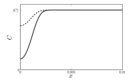
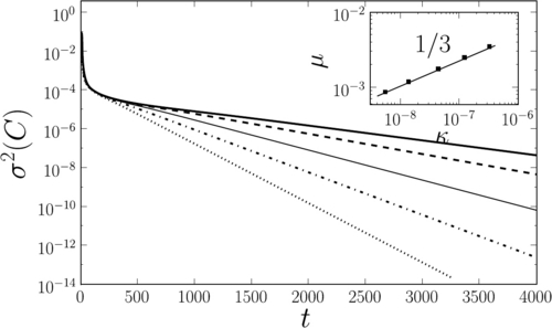
Figure 10: (a) Structure of the eigenmode: an inverted half-Gaussian of width $w_{0}$ decays exponentially at a rate $-\log(g_{1}^{\prime}(w_{0}))=2aw_{0}$. (b) Concentration variance measured in the whole unit interval $[0,1]$ for different diffusivities. (The thick solid, dashed, solid, dot-dashed and dotted lines correspond respectively to the following values of $\kappa$: $5.4\times 10^{-9}$, $1.3\times 10^{-8}$, $4.3\times 10^{-8}$ $1.2\times 10^{-7}$ and $3\times 10^{-7}$.) For long times, the evolution of the variance is exponential, corresponding to the onset of a eigenmode: $\sigma^{2}(C,t)=\sigma^{2}_{0}\exp(-\mu t)$. As expected from Eq. (32), $\mu$ scales as $\kappa^{1/3}$ (inset).

Once the concentration at $x=0$ starts rising, which occurs for $d(t)=1/at\sim w_{0}$ (i.e. $350$ periods for a diffusivity $\kappa=10^{-7}$!), the stabilized half-Gaussian decays exponentially at a rate $-\log(g_{1}^{\prime}(w_{0}))=2aw_{0}$, which scales as $\kappa^{1/3}$. We have verified this scaling in numerical simulations of the model (see Fig. 10(b)). Note that this is one of the very few examples where one can predict analytically the decay of a eigenmode (another noteworthy situation is the torus map considered in Ref. Thiffeault and Childress (2003)). However, this eigenmode regime is not relevant in practice, as we only observe it when fluctuations are completely negligible in the bulk. Its structure is also quite trivial: it consists of the half-Gaussian at $x=0$, and of very small spikes centered on the iterates of $x=0$ in the bulk.

The convergence to the eigenmode can be interpreted as follows. Once the mixing pattern reaches the diffusive layer $w_{0}$ at the boundary, every box with size equal to the local diffusive scale contains an iterate of the initial blob of dye. A global decay of the concentration variance is therefore possible from then on.

V.2 Other initial conditions

For the sake of completeness, we have performed numerical simulations for other initial conditions than a blob of dye. In particular, we have simulated two different situations, a cosine profile, corresponding to an initial condition

$$C(x,t=0)=1+\cos(4\pi x),$$ (33)

and a random profile where we attribute to each pixel a random value between 0 and 1. This rapidly varying profile is quickly smoothed everywhere on the local Batchelor scale. The main difference between the two initial conditions may be assessed as follows. For the cosine profile, the initial scale of variation for the scalar field is much greater than the Batchelor scale at the boundary $w_{0}$, whereas for the random initial condition, the scalar field already varies on the smallest possible scales.

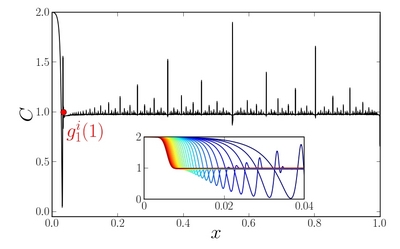
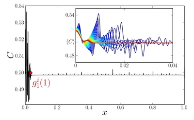
Figure 11: [Color online] Homogenization for two different initial conditions: (a) $C(x,t=0)=1+\cos(4\pi x)$, (b) random initial profile. The scale of variation of the initial profile is much greater than $w_{0}$ in the first case, whereas it is of order $w_{0}$ close to the boundary in the random case. Main axes: concentration profile after 30 iterations of the map. Note that all variance is contained in the leftmost image of the unit interval (always transformed by $g_{1}$), and around the iterates of $x=1$. Inset: zoom on the border region for periods 30 (dark blue) to 180 (red), represented every fifth period.

In the first case, as for the blob of dye, the scale of variation of the profile close to the boundary is large, of order $g^{t}_{1}(1)\sim 1/(at)$ (see inset of Fig. 11(a)). This case is therefore analogous to the blob of dye case. After a short time, most important fluctuations are concentrated in the leftmost image of the initial unit interval, that was iterated only by $g_{1}$. Other iterates have wandered in the bulk where stretching is much more efficient, so that all fluctuations have died out — except for newly-reinjected iterates. The history of newly-reinjected iterates can be coded as a sequence $G\circ g_{1}\circ g_{2}\circ g_{1}^{k}$ where $G$ stands for the last few iterations, which corresponds to the reinjection inside the bulk of fluctuations at the left boundary. Even the leftmost iterate feels the spatial heterogeneity of stretching (see inset in Fig. 11(a)), as fluctuations initially close to $x=1$ have been more compressed, and they have overlapped and averaged. After some time, the profile at the boundary (inset in Fig. 11(a))) has a value significantly different from the mean concentration only at one or two “oscillations”, which is exactly what we observe for the blob of dye case (see Fig. 6). As in the latter case, we observe a power-law decay for the variance evolution, which can be accounted for by the same reasoning.

For the random profile case, the concentration profile at the boundary (inset in Fig. 11(b)) is much less coherent over successive periods. Indeed, the scale of variation of the concentration profile saturates immediately at the local Batchelor scale in the whole domain. The strips reinjected in the bulk result from the averaging of many strips at the boundary, and their amplitude is more difficult to predict. We measured a non-monotonic decay of variance inside the bulk in this case, as the averaging of strips close to the wall depends on the instantaneous height of many neighboring strips (Fig. 11(b)). Yet, the strange eigenmode regime is only reached once fluctuations have died out everywhere, except for the leftmost box of size $w_{0}$ and around the iterates of $x=0$, so that there is a long transient phase also in this case.

However, many features are common to all initial conditions that we checked. The spatial organization of the bulk profile is dominated by the unstable manifold of the parabolic point at $x=0$, where fluctuations persist longer. As stretching is lower close to the boundary, the reinjected fluctuations are similar over successive periods. The same reasoning as for the blob of dye yields concentration PDFs with power-law tails of the form $|C-\langle C\rangle|^{-2}$, which are indeed observed in all cases.

V.3 Hydrodynamical optimization

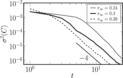
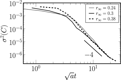
Figure 12: (a) Evolution of the concentration variance in a large central domain for three different versions of the figure-eight protocol, corresponding to $r_{\infty}=0.24,\,0.3$ and $0.38$, obtained by advecting Lagrangian particles in Stokes-flow numerical simulations. (b) Evolution of the concentration variance for the same protocols vs time rescaled by the parameter $\sqrt{a}$ ($r_{\infty}=0.24,\,0.3$ and $0.38$ correspond respectively to $a=0.39,0.72$ and $1.39$). A satisfying collapse of all curves is observed.

We have argued that for a wide class of mixing protocols the decay of the concentration initially obeys a power law. For industrial devices, it is of primary importance to optimize the decay during this initial phase, that is, to tune the prefactor in the power law. Our analysis in Section IV shows that the prefactor is essentially determined by the parameter $a$, which controls the evolution of the distance between the mixing pattern and the wall in Eq. (10). (The exponent of the power law also depends weakly on the mean stretching $\Gamma$.)

We check the validity of the parametrization of the variance by the rate $a$ for the figure-eight protocol. As for the blinking vortex protocol, we follow a large number of particles, in order to record the evolution of a coarse-grained concentration field. We perform numerical simulations of a Stokes-flow version of the figure-eight protocol, for different values of the radius of the figure-eight loops $r_{\infty}$. In all cases, the initial condition is a small square of size $0.1\times 0.1$ located close to the rod and containing $2.25\times 10^{6}$ particles. We calculate the variance of the concentration on a large half-crown of outer radius $0.8$. We show results for the evolution of the variance in Fig. 12 (a). For $r_{\infty}=0.24,\,0.3$ and $0.38$, we observe a power-law evolution with an exponent close to $4$, but slightly greater for the smallest radius $r_{\infty}=0.24$. Numerical simulations do not permit the same spatial resolution as in experiments; we use a coarse-graining scale $w_{\mathrm{B}}=10^{-2}$. Measuring the distance of the mixing pattern to the wall, we deduce the values of $a$ and $\tau_{\mathrm{W}}$. Using this coarse spatial resolution and for each value of $a$, we compute $\tau_{\mathrm{W}}\sim 5$. The evolution of the variance in Fig. 12 is therefore in agreement with the $-4$ exponent of the variance determined in Sec. IV for the regime $t>\tau_{\mathrm{W}}$. The larger exponent for the smallest radius could be attributed to a weaker mean stretching $\Gamma$ in this case, since the rod travels in a smaller region.

In our model, the dependence of the variance on the details of the protocol comes from the factor $\Delta^{2}(t)\simeq(\sqrt{a}t)^{-4}$ in the regime $t>\tau_{\mathrm{W}}$. We have plotted in Fig. 12 (b) the evolution of the variance against the rescaled time $\sqrt{a}t$. We observe a very good collapse of all data on the same curve, supporting the idea that the main ingredient in the evolution of the variance is the parameter $a$.

Increasing the mixing speed therefore amounts to increasing the rate $a$ at which a particle approaches the wall. This can be achieved in a number of ways, such as increasing the rod diameter or by “scraping the bowl”, that is taking the stirrers closer to the wall as in Fig. 12. Determining the value of $a$ as a function of hydrodynamic parameters such as the rod diameter or the size of the rod’s orbit is beyond the scope of this article. However, our results suggest that in comparing different mixing protocols the rate $a$ gives a simple estimate of the variance decay rate and can replace more challenging measurements, such as the concentration field itself.

V.4 Conclusions

The results of this paper can be summarized as follows. Using an approach based on the Lagrangian description of fluid particles stretched into filaments, we have highlighted the role of least-unstable periodic structures in mixing dynamics, first in the well-known baker’s map, and then for a broad class of 2-D closed flows where the chaotic region extends to a no-slip wall. For the latter class of systems, we have proposed a generic scenario for wall-dominated mixing dynamics. No-slip hydrodynamics in the wall region force poorly-mixed fluid to be slowly reinjected in the bulk along the unstable manifold of a parabolic point. (Note that phase portraits with many injection points are also possible. This does not affect the validity of our arguments.) Mixing dynamics are then controlled by the slow stretching at the wall, which contaminates the whole mixing pattern up to its core. We observed a slow algebraic decay of the concentration variance in experiments and numerical simulations, which we justified analytically using a 1-D model of a baker’s map with a parabolic point on the boundary. An exponential decay corresponding to an eigenmode is recovered in the model once iterates of the initial blob of dye are present in all boxes of size of the local diffusive scale, that is for extremely long times at which the variance has been almost completely exhausted.

We characterize a mixing experiment by the following parameters: the flow’s mean compression factor $\Gamma$; the algebraic rate $a$ at which a particle approaches the boundary; the Batchelor scale $w_{\mathrm{B}}$ obtained from the diffusivity $\kappa$ and compression $\Gamma$; and the width of the initial blob $\delta$. The successive stages of the mixing process inside the bulk can be summarized as follows.

• For $t<\log\left(w_{\mathrm{B}}/\delta\right)/\log\Gamma$, all filaments are larger than $w_{\mathrm{B}}$ and the variance is constant: $\sigma^{2}(C)=\sigma^{2}_{0}$.

• For $\log\left(w_{\mathrm{B}}/\delta\right)/\log\Gamma\leq t\leq\left(aw_{\mathrm{B}}\right)^{-1/2}$, fluctuations in the bulk start to decay as dye filaments are compressed below $w_{\mathrm{B}}$, and the variance is dominated by large unmixed strips recently injected from the near-wall region into the bulk: $\sigma^{2}\propto\delta^{2}\times(\log{at^{2}}+\log{w_{\mathrm{B}}})/(a\log{\Gamma}\times t^{2})$, as derived in Sec. IV.1.

• For $\left(aw_{\mathrm{B}}\right)^{-1/2}\leq t\leq(\kappa/4a)^{1/3}$, all reinjected strips are smaller than $w_{\mathrm{B}}$, yet their contribution still dominates the variance evolution $\sigma^{2}\propto 1/(a^{2}t^{4})$. This scaling was derived in Sec IV.2.

• For $t\geq(\kappa/4a)^{1/3}$, we are in the eigenmode regime (see Sec. V.1) and $\sigma^{2}\propto\exp(-\mu t)$, where $\mu\propto(\kappa a^{2})^{1/3}$.

Our study has highlighted the role of periodic structures with lowest stretching in the construction of a time-persistent mixing pattern, dominated by their unstable manifold. This applies to the least-unstable periodic point in the baker’s map (thus a hyperbolic point) and to the wall parabolic point for the figure-eight case. The importance of elliptic region for limiting mixing dynamics has been emphasized in other studies Pikovsky and Popovych (2003); Popovych et al. (2007).

In 2-D flows, where Lagrangian dynamics are Hamiltonian, the wall region can either belong to a chaotic region, or to an elliptical island. We have argued that algebraic mixing dynamics are obtained in the first case. An experimental study of mixing dynamics in the second case is in preparation and will be reported elsewhere.

Acknowledgments

Natalia Kuncio took an important part in the figure-eight experiments. The authors also would like to thank Cécile Gasquet and Vincent Padilla for technical assistance, as well as François Daviaud, Emmanuel Villermaux and Philippe Petitjeans for fruitful discussions.

References

- Aref (1984) H. Aref, J. Fluid Mech. 143, 1 (1984).
- Ottino (1989) J. M. Ottino, The Kinematics of Mixing: Stretching, Chaos, and Transport (Cambridge University Press, Cambridge, U.K., 1989).
- Pierrehumbert (1994) R. T. Pierrehumbert, Chaos Solitons Fractals 4, 1091 (1994).
- Fereday et al. (2002) D. R. Fereday, P. H. Haynes, A. Wonhas, and J. C. Vassilicos, Phys. Rev. E 65, 035301 (2002).
- Wonhas and Vassilicos (2002) A. Wonhas and J. C. Vassilicos, Phys. Rev. E 66, 051205 (2002).
- Sukhatme and Pierrehumbert (2002) J. Sukhatme and R. T. Pierrehumbert, Phys. Rev. E 66, 056302 (2002).
- Pikovsky and Popovych (2003) A. Pikovsky and O. Popovych, Europhys. Lett. 61, 625 (2003).
- Thiffeault and Childress (2003) J.-L. Thiffeault and S. Childress, Chaos 13, 502 (2003).
- Fereday and Haynes (2004) D. R. Fereday and P. H. Haynes, Phys. Fluids 16, 4359 (2004).
- Thiffeault (2004) J.-L. Thiffeault, Chaos 14, 531 (2004).
- Liu and Haller (2004) W. Liu and G. Haller, Physica D 188, 1 (2004).
- Haynes and Vanneste (2005) P. H. Haynes and J. Vanneste, Phys. Fluids 17, 097103 (2005).
- Antonsen et al. (1995) T. Antonsen, Z. F. Fan, and E. Ott, Phys. Rev. Lett. 75, 1751 (1995).
- Antonsen and Ott (1996) T. Antonsen and E. Ott, Phys. Fluids 8, 3094 (1996).
- Ott and Antonsen (1989) E. Ott and T. M. Antonsen, Phys. Rev. A 39, 3660 (1989).
- Antonsen and Ott (1991) T. Antonsen and E. Ott, Phys. Rev. A 44, 851 (1991).
- Rothstein et al. (1999) D. Rothstein, E. Henry, and J. P. Gollub, Nature (London) 401, 770 (1999).
- Jullien et al. (2000) M.-C. Jullien, P. Castiglione, and P. Tabeling, Phys. Rev. Lett. 85, 3636 (2000).
- Voth et al. (2003) G. Voth, T. Saint, G. Dobler, and J. Gollub, Phys. Fluids 15, 2560 (2003).
- Gilbert (2006) A. D. Gilbert, Dynamical Systems 21, 25 (2006).
- Chertkov and Lebedev (2003) M. Chertkov and V. Lebedev, Phys. Rev. Lett. 90, 034501 (2003).
- Lebedev and Turitsyn (2004) V. V. Lebedev and K. S. Turitsyn, Phys. Rev. E 69, 036301 (2004).
- Schekochihin et al. (2004) A. Schekochihin, P. Haynes, and S. Cowley, Phys. Rev. E 70, 46304 (2004).
- Salman and Haynes (2007) H. Salman and P. H. Haynes, Phys. Fluids 19, 067101 (2007).
- Burghelea et al. (2004) T. Burghelea, E. Segre, and V. Steinberg, Phys. Rev. Lett. 92, 164501 (2004).
- Gouillart et al. (2007) E. Gouillart, N. Kuncio, O. Dauchot, B. Dubrulle, S. Roux, and J.-L. Thiffeault, Phys. Rev. Lett. 99, 114501 (2007).
- Balkovsky and Fouxon (1999) E. Balkovsky and A. Fouxon, Phys. Rev. E 60, 4164 (1999).
- Thiffeault (2008) J.-L. Thiffeault, in Transport and Mixing in Geophysical Flows, edited by J. B. Weiss and A. Provenzale (Springer, Berlin, 2008), vol. 744 of Lecture Notes in Physics, pp. 3–35, eprint arXiv:nlin/0502011.
- Villermaux and Duplat (2003) E. Villermaux and J. Duplat, Phys. Rev. Lett. 91, 184501 (2003).
- Pierrehumbert (2000) R. T. Pierrehumbert, Chaos 10, 61 (2000).
- Farmer et al. (1983) J. D. Farmer, E. Ott, and J. A. Yorke, Physica D 7, 153 (1983).
- Tél et al. (2000) T. Tél, G. Károlyi, A. Péntek, I. Scheuring, Z. Toroczkai, C. Grebogi, and J. Kadtke, Chaos 10, 89 (2000).
- Venaille and Sommeria (2007) A. Venaille and J. Sommeria, Phys. Fluids 19, 028101 (2007).
- Popovych et al. (2007) O. V. Popovych, A. Pikovsky, and B. Eckhardt, Phys. Rev. E 75, 036308 (2007).
- Jana et al. (1994) S. C. Jana, G. Metcalfe, and J. M. Ottino, J. Fluid Mech. 269, 199 (1994).
- Finn and Cox (2001) M. D. Finn and S. M. Cox, Journal of Engineering Mathematics 41, 75 (2001).
- Mezić (2001) I. Mezić, J. Fluid Mech. 431, 347 (2001).
- Haller (2004) G. Haller, J. Fluid Mech. 512, 257 (2004).