Low heat conduction in white dwarf boundary layers ?

Abstract

Context. X-ray spectra of dwarf novae in quiescence observed by Chandra and XMM-Newton provide new information on the boundary layers of their accreting white dwarfs.

Aims. Comparison of observations and models allows us to extract estimates for the thermal conductivity in the accretion layer and reach conclusions on the relevant physical processes.

Methods. We calculate the structure of the dense thermal boundary layer that forms under gravity and cooling at the white dwarf surface on accretion of gas from a hot tenuous ADAF-type coronal inflow. The distribution of density and temperature obtained allows us to calculate the strength and spectrum of the emitted X-ray radiation. They depend strongly on the values of thermal conductivity and mass accretion rate.

Results. We apply our model to the dwarf nova system VW Hyi and compare the spectra predicted for different values of the thermal conductivity with the observed spectrum. We find a significant deviation for all values of thermal conductivity that are a sizable fraction of the Spitzer conductivity. A good fit arises however for a conductivity of about 1% of the Spitzer value. This also seems to hold for other dwarf nova systems in quiescence. We compare this result with thermal conduction in other astrophysical situations.

Conclusions. The highly reduced thermal conductivity in the boundary layer requires magnetic fields perpendicular to the temperature gradient. Locating their origin in the accretion of magnetic fields from the hot ADAF-type coronal flow we find that dynamical effects of these fields will lead to a spatially intermittent, localized accretion geometry at the white dwarf surface.

1 Introduction

Cataclysmic variables (CVs) are interacting binaries in which mass flows from a low mass companion star and accretes on the white dwarf primary. The X-ray emission of the large number of cataclysmic variables makes up a large fraction of the apparently diffuse Galactic Ridge X-ray emission, as was recently found with the help of deep surveys by Chandra and XMM-Newton (Sazonov et al. 2006). In dwarf nova systems, non-magnetic CVs, the accretion onto the white dwarf occurs via an accretion disk and the gas must dissipate its rotational kinetic energy before it settles on the surface of the more slowly rotating white dwarf. The X-ray emission is thought to originate from the interface between the white dwarf and the inner edge of the disk, a boundary layer close to the surface. The disk is too cool to contribute significantly to the X-ray emission.

Different models have been proposed for the structure of the X-ray emitting region in dwarf nova at low accretion rates, i.e. in their quiescent state: (1) a cooling flow model based on Mushotzky & Szymkowiak (1988), which assumes isobaric radiative cooling of the gas; (2) a model of a hot boundary layer where heat advection is dominant (Narayan & Popham 1993); (3) a thermal boundary layer model where heat conduction determines the structure of the spherically accreting gas around the white dwarf (Liu, Meyer & Meyer-Hofmeister 1995) and a similar X-ray emitting corona model of Mahasena & Osaki (1999); and (4) hot settling flow solutions ( Narayan & Medvedev 2001, Medvedev & Menou 2002) in which viscously mediated losses of rotational energy are an important parameter. In these papers references to earlier discussions of emission mechanisms are given.

The much improved sensitivity and spectral resolution of the new X-ray telescopes allow us to test specific models. The first tests were performed by Pandel et al. (2003) for VW Hyi in quiescence and by Perna et al. (2003) for WX Hydri in quiescence. Pandel et al. (2003) used X-ray and ultraviolet data obtained with XMM-Newton. The authors found that the X-ray spectrum indicates the presence of optically thin plasma in the boundary layer that cools as it settles on the white dwarf, and that the plasma has a range of temperatures that is well described by a power law or a cooling flow model with a maximum temperature of 6-8 keV. Perna et al. (2003) used Chandra observations for their investigation, computed spectra for the available theoretical models, i.e. hot boundary layers, hot settling flows and X-ray emitting coronae. They came to the conclusion that the continuum is reproduced well by most of the models, but none of them can fully account for the relative line strengths over the entire spectral range. Pandel et al. (2005) studied 10 dwarf novae, based on XMM-Newton observations, including the earlier results for VW Hyi by Pandel et al. (2003). The authors conclude that the X-ray emission originates from a hot, optically thin multi-temperature plasma with a temperature distribution in close agreement with an isobaric cooling flow, pointing to a cooling plasma settling onto the white dwarf as the source of X-rays.

We use the model description worked out earlier (Liu et al. 1995), which is related to the “siphon flow model” for a corona above an accretion disk in quiescence (Meyer & Meyer-Hofmeister 1994). In this picture matter in the innermost disk is evaporated into a coronal flow which provides a geometrically thick gas flow towards and around the white dwarf. (Dwarf nova systems have cycles of longer lasting quiescent phases and shorter outbursts. These outbursts are triggered by a disk instability, then the matter accumulated in the disk during quiescence accretes with a high mass flow rate onto the white dwarf (Meyer & Meyer-Hofmeister 1984). For the formation of the inner disk hole see Liu et al. (1997)). Since the flow of gas from the surrounding corona is an essential feature of our model our approach differs from the simulation of the boundary layer between a white dwarf and a thin accretion disk which extends all the way down to the stellar surface, as studied recently by Balsara et al. (2007). These numerical simulations give insight into the spreading of the boundary layer, but no conclusions on spectra are derived.

We have chosen the well documented dwarf nova VW Hyi for our new investigation. We compute the thermal boundary layer structure, evaluate the emission measures and determine spectra using the XSPEC package. We come to the somewhat surprising result that only structures based on very low conductivity give spectra in agreement with the observations. Pandel et al. (2005) already remarked that heat conduction does not dominate over cooling via X-ray emission because otherwise $T_{\rm{max}}$, the initial temperature of the cooling gas, would be much smaller than the virial temperature$T_{\rm{vir}}$ (the temperature the gas would have if all the rotational energy from its Keplerian motion were instantly converted into heat). Indeed high temperatures are needed to obtain a spectrum such as the one observed for VW Hyi. The aim of our paper is to study the structure of the boundary layer under heat conduction. We discuss what might cause low heat conduction that seems different from heat conduction in other astrophysical situations. As the analysis of thermal conduction in clusters of galaxies by Narayan and Medvedev (2001) shows, a low conductivity would point to a non-chaotic magnetic field.

In Sect. 2 we describe the observations we use for our comparison. In Sect. 3 we briefly discuss the physics entering our structure computations as well as the boundary conditions at the bottom and the top of the boundary layer. We compare different models in Sect. 4. In Sect. 5. the results of the structure computations are presented, in Sect. 6 the evaluated spectra. We argue that the spectra of other dwarf novae also indicate low thermal conductivity in these systems. We discuss the presence of low or high thermal conductivity indicated in different astrophysical sources as clusters of galaxies and the intercluster medium (Sect. 7). The low conductivity found here possibly indicates an important role of the magnetic field in the boundary layer accretion process. Our conclusions follow in Sect. 8.

2 X-ray observations

For the comparison of our theoretical spectra with observation we use the XMM-Newton spectrum (Jansen 2001) of VW Hyi obtained with the European Photon Imaging Camera (EPIC) (Strüder et al. 2001). This system was observed with the EPIC-pn in full-frame mode on 2001 October 19 for 16.1 ks, from 06:10:05 to 10:38:34, in quiescent state, 22 days after a normal outburst and 23 days before the next outburst (which was a superoutburst). The spectrum was extracted using SAS version. The observed spectrum is shown in Fig. 5. The same data for VW Hyi have also been used by Pandel et al. (2003) and were included in the work by Pandel et al. (2005).

3 The boundary layer structure

We describe the accretion process through the boundary layer around the white dwarf mainly as presented in an earlier work (Liu et al. 1995). Passing through a turbulent region, the accreting matter totally loses its angular momentum, becomes subsonic and forms a layer around the white dwarf. We assume that the density is higher towards the equatorial plane, so that accretion occurs onto a belt around the white dwarf. We assume that its area is about half of the full stellar surface area. We take spherical coordinates with $r$ the distance to the white dwarf center , $r_{*}$ the white dwarf radius, and $S=r_{*}-r$ the height above the white dwarf surface (negative sign). The downward directed thermal conductive flux is

$$F_{c}=-\kappa_{0}\,T^{5/2}\,\frac{dT}{dS}$$ (1)

with $T$ temperature, $\kappa_{0}$ thermal conductivity coefficient, taken as the standard value $\kappa_{\rm Sp}=10^{-6}\rm{gcm/(sec^{3}\bf{(K)}^{7/2})}$ (Spitzer 1962). Heat conduction is an important feature in the model, different to a cooling flow model. We evaluate the structure for different values of the thermal conductivity $\kappa_{0}$, 1/5, 1/25 and 1/100 of $\kappa_{\rm Sp}$. Mass conservation gives

$$\dot{M}=2\pi r^{2}\rho v=const.$$ (2)

with $\dot{M}$ accretion rate, $\rho$ density and $v$ flow velocity (positive if downward directed). Euler’s equation in the stationary case is

$$v\frac{dv}{dS}+\frac{1}{\rho}\frac{dP}{dS}-\frac{GM_{*}}{r^{2}}=0$$ (3)

with $P$ pressure, $G$ gravitational constant, $M_{*}$ mass of the white dwarf. Energy conservation gives

$$\frac{1}{r^{2}}\frac{d}{dS}\>\left[\frac{\dot{M}}{2\pi}\left(\frac{1}{2}v^{2}+\frac{GM_{*}}{r_{*}}-\frac{GM_{*}}{r}+\frac{\gamma}{\gamma-1}\frac{P}{\rho}\right)+r^{2}F_{c}\right]$$ (4)

$$=-\Lambda(T)\>n_{e}\,n$$

with $\gamma=\frac{5}{3}$ the ratio of specific heats for the fully ionized gas, atom and electron densities $n$, $n_{e}$ and $\Lambda(T)$ the radiative loss function for solar abundance (Sutherland & Dopita 1993). In our highly subsonic solutions the kinetic energy term is negligibly small.We have normalized the gravitational potential energy to zero at the white dwarf surface. (Following Shmeleva $\&$ Syrovatskii (1973) we had added a source term to account for the finite surface temperature of the white dwarf, see Liu et al. (1995)). We solve these equations together with the equation of state.

We assume that before radiative losses of the settling gas become important, the accretion flow has already lost its angular momentum, with which it started from the corona at the disk truncation radius, and that the rotational energy has been dissipated into heat. The maximum energy which this flow can bring with it is then the gravitational energy between the disk truncation radius and the white dwarf surface where the former term can be neglected if the truncation radius is many white dwarf radii away. Support for our neglect comes from the boundary layer rotation velocities derived by Pandel et al. (2005) for the dwarf novae in their sample, found to be considerably smaller than the Keplerian velocity near the white dwarf.

Our boundary conditions are the following. The lower boundary is located at the white dwarf surface. The temperature is taken equal to the black body temperature arising from the irradiation of the surface by the downward directed half of the radiative energy release. For the location of the upper boundary we take a height above the white dwarf surface above which the radiative loss is negligible. At this height we require that the total energy flow, i.e. the sum of advective, gravitational and thermal conductive flow, equals the total available accretion energy flow. These energies are

$$\dot{E}_{\rm{conductive}} = 2\pi r^{2}F_{c}$$ (5)

$$\dot{E}_{\rm{advective}} = \dot{M}\,\frac{\gamma}{\gamma-1}\frac{\Re}{\mu}T$$ (6)

$$\dot{E}_{\rm{gravitational}} = \dot{M}\,\frac{GM}{r_{*}}\left(\frac{1}{r_{*}}-\frac{1}{r}\right)$$ (7)

with $\Re$ gas constant and $\mu$ molecular weight (taken as 0.6).

This boundary condition neglects outward conductive heat losses at large radii where the temperature drops outwards. Such losses have been estimated to be small in Liu et al. (1995) where they amount, for full Spitzer conductivity, to the order of magnitude of the evaporation energies at large radii. (Real temperatures would come out slightly lower than with this neglect.) After taking the mass accretion rate that corresponds to the observed flux, our model contains no free parameter except the assumed value of thermal conductivity, which we want to test.

4 Comparison of different models

In an isobaric cooling flow (Mushotzky & Szymkowiak 1988) the emission measure for each temperature decrement is determined by the time it takes the matter to radiatively cool down to the next temperature shell. No thermal conductivity is included. To simulate the observed spectrum a mass flow rate that corresponds to the observed flux is taken, in addition as a free parameter a maximal temperature is chosen to fit the observations.

Narayan and Popham (1993) investigated the structure of thin accretion disks around a central white dwarf with emphasis on a self-consistent description of the boundary layer. The decrease of rotation from the Keplerian value at the upper boundary to the value at the stellar surface as well as friction is taken into account. For low rates as appropriate for the dwarf nova systems in quiescence they found an optically thin very hot boundary layer. Heat is transported advectivily into the optically thick layers of the white dwarf from where it is radiated as X-rays. These investigations are carried out only for accretion rates 10 times higher or even more than in our VW Hyi analysis.

The solutions based on a hot settling flow by Medvedev & Narayan (2001) and Medvedev & Menou (2002) also include the rotational energy of the accreting gas, so that the white dwarf rotation and the viscous nature of the flow are accounted for. Mahasena & Osaki (1999) model the boundary layer structure as determined by thermal conduction in the settling gas around the white dwarf, similar to the ’siphon-flow model’ for a disk corona (Meyer & Meyer-Hofmeister 1994), and also similar to our white dwarf boundary modeling.

5 Results of computations

5.1 Energy flows in the boundary layer

We solve the system of differential equations given in the previous section, the same procedure as carried out for the earlier investigation (Liu et al.1995). For our comparison of theoretical and observed spectra for VW Hyi we take $0.62M_{\odot}$ for the white dwarf mass and $8.3\cdot 10^{8}$ cm for its radius. We do not perform computations for different abundances since the aim of our analysis is the study of the influence of thermal conductivity. The change of abundances allows better fits of the observed spectrum. For a discussion of the abundances present in VW Hyi see the discussion in Pandel et al. (2005). The free parameter in our model is the mass accretion rate. We take $\dot{M}=1.25\>10^{-12}M_{\odot}/yr$ assuming that the matter is accreted on an equatorial belt covering half of the white dwarf surface area. Because we find that 100% the Spitzer value does not give an acceptable agreement with the observations, we vary the value of heat conductivity. In the following we show results for 1/100 and 1/25 and 1/5 of the standard Spitzer value.

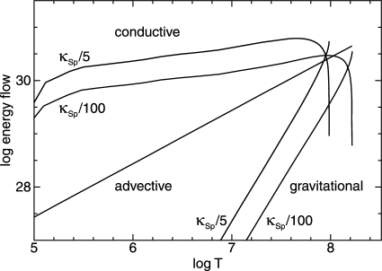
Figure 1: Energy flux versus temperature for heat conductivity 1/5 and 1/100 of the Spitzer value. Note the higher temperature maximum, $1.6\cdot 10^{8}$ K, for the lower conductivity value

In Fig. 1 we show the evaluated change of energy flows with increasing height, that is increasing temperature for a heat conduction reduced to 1/5 and 1/100 of the standard value. The upper boundary location (according to the requirements discussed in the last section) is at different heights above the white dwarf surface, at $6.8\cdot 10^{8}$ cm in the first case and $1.8\cdot 10^{9}$ cm in the second case. For the lower conductivity the advective energy is dominant at high temperature. The most important difference is the maximum temperature reached. This has a strong influence on the resulting emission measures (and the spectrum) as will be shown later. In our model the maximum temperature is a result of the structure computations. Note that in the cooling flow model the maximal temperature is chosen to fit the spectrum.

5.2 Emission measures

In Fig.2 differential emission measures (emission measures per $\rm{cm^{2}}$ surface area, per degree) [$\rm{cm^{-5}K^{-1}}$] are shown for a heat conductivity 1/5 and 1/100 of the standard Spitzer value. For the higher value of heat conductivity the differential emission measures are systematically higher, but with no contribution at high temperature.

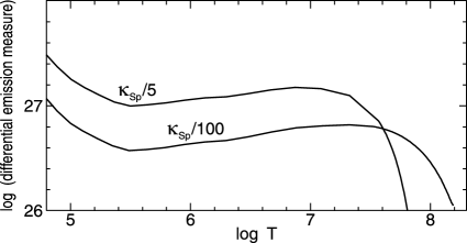
Figure 2: Differential emission measures per surface area [$\rm{cm^{-5}K^{-1}}$] for heat conductivity 1/5 and 1/100 of the standard Spitzer value.

To obtain the radiation from the boundary layer, the differential emission measures have to be multiplied by the area from which the radiation comes, the temperature $T$ and the cooling function $\Lambda(T)$. The surface area is the spherical shell around the white dwarf at the height with temperature $T$. Since all the boundary layer is close to the white dwarf this flaring effect in the geometry only occurs at the highest temperatures. This product, the evaluated contributions to the luminosity from different temperature regions, is shown in Fig.3. The departure from smooth lines is due to the non-smooth dependence of the cooling function on temperature. With this display of luminosity distributions it becomes clear that different contributions arise from the structure at high temperatures. And, as shown in the next section, agreement with the observed spectrum for VW Hyi can only be gained with the high temperature contributions which result from the low conductivity.

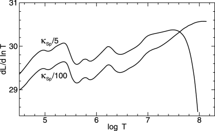
Figure 3: Total emission per logarithmic temperature interval for heat conductivity 1/5 and 1/100 of the standard Spitzer value.

The emission measures of a cooling flow model are (see Pandel et al. 2005, taken from Mushotzky & Szymkowiak 1988)

$$\frac{dEM}{dT}=\frac{5}{2}\frac{\Re}{\mu}\dot{M}\frac{n^{2}}{\varepsilon(T,n)}$$ (8)

with $\varepsilon(T,n)$ the total emissivity per volume. The total emission per logarithmic temperature then becomes $dEM/dT\>\Lambda(T)\,T=\frac{5}{2}\frac{\Re}{\mu}\dot{M}T$. Pandel et al. (2005) modified the cooling flow model emission measures adding a factor $\left(T/T_{\rm{max}}\right)^{\alpha}$, with $\alpha$=-0.05 for VW Hyi to improve the fit of the spectrum, and derived an accretion rate of $3.7\cdot 10^{-12}\>\rm{M_{\odot}/yr}$. We use $1.25\cdot 10^{-12}\>\rm{M_{\odot}/yr}$ for our calculation, the matter accreting onto half the white dwarf surface. To compare the cooling flow radiation with our results for low conductivity we have multiplied these cooling flow emission measures (without $\alpha$ modification) by a factor of 0.676 (=ratio of accretion rates, our rate doubled) to account for the different accretion rates and accretion areas. The result is shown in Fig.4. The contributions from the cooling flow model lie above those from our model, but end at the maximum temperature chosen for the fit, $T_{\rm{max}}=9.5\cdot 10^{7}$ K, so the emission is roughly compensated.

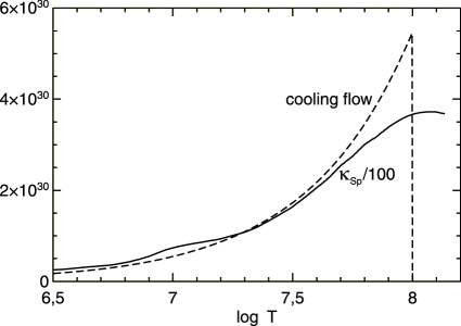
Figure 4: Comparison of total emission per logarithmic temperature interval for a cooling flow model and our model for low conductivity

6 Spectra

We use the X-ray spectral fitting package XSPEC (version 11). We evaluated the spectra for the three sets of boundary layer structure computed for the conductivity 1/5, 1/25 and 1/100 of the standard Spitzer value. We show these spectra in Fig. 5 (a), (b), and (c). The spectra document how the thermal conductivity determines the distribution of radiation over the energy range. A comparison of Fig. 3 shows how the different contributions to the radiation for high and low conductivity values determine the spectrum for temperatures around $10^{7}$ and $10^{8}$. Below each spectrum the $\chi$-statistics values are shown. Note the different scales in Fig. 5 (a), (b), and (c). Only for the low conductivity do we find an acceptable agreement.

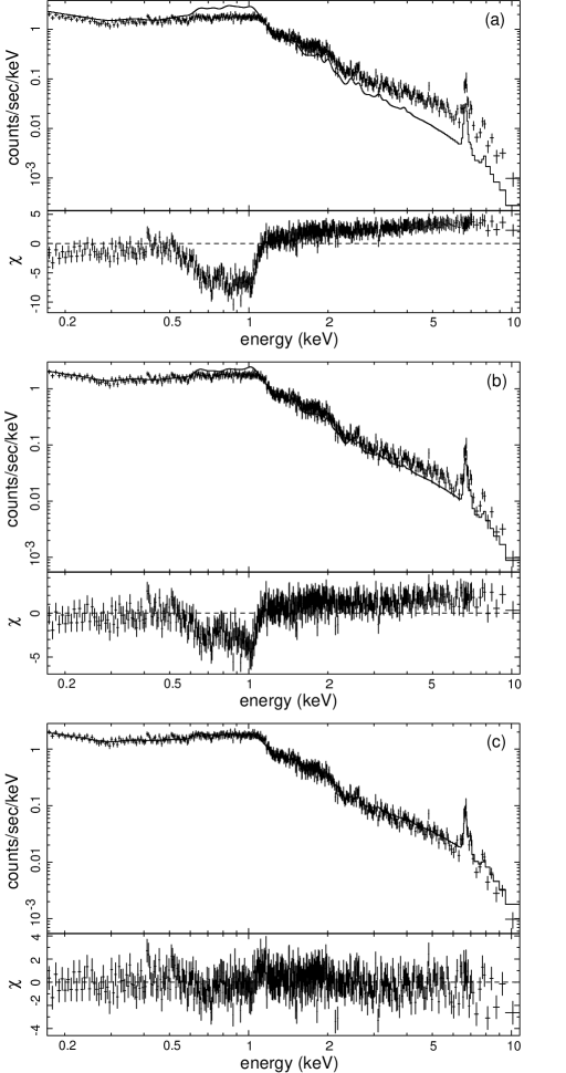
Figure 5: Comparison of XMM-Newton EPIC spectra for VW Hyi in quiescence with model spectra evaluated for an accretion rate of $\dot{M}=1.25\cdot 10^{-12}\,\rm{M_{\odot}/yr}$ and for different thermal conductivity: (a) $1/5\kappa_{\rm{Sp}}$, (b) $1/25\kappa_{\rm{Sp}}$ and (c) $1/100\kappa_{\rm{Sp}}$.

We have not tried to obtain the best fit for a variation of the mass accretion rate, nor for changes of the abundances, and we have not analyzed spectral lines, as was done in previous work (Pandel et al. 2003, Perna et al. 2003, Pandel et al. 2005). The aim of our investigation is to study the influence of the heat conductivity.

We compare the accretion rate roughly found from our modeling, $1.25\cdot 10^{-12}\,\rm{M_{\odot}/yr}$, with the rates derived in other investigations. Pandel et al. (2003) found $5\cdot 10^{-12}\,\rm{M_{\odot}/yr}$ and Pandel et al. (2005) $3.7\cdot 10^{-12}\,\rm{M_{\odot}/yr}$, for fits to the same data. Previous observations for VW Hyi lead to an estimate of $3\cdot 10^{-12}\,\rm{M_{\odot}/yr}$ for the accretion rate in late quiescence (BeppoSAX observations by Hartmann et al. 1999); similar results were gained from earlier observations (EXOSAT and ROSAT observations by van der Woerd et al. 1987, Belloni et al. 1991). From theoretical arguments one would expect that the X-ray flux changes during the quiescent interval in the outburst cycle. One would expect an increase of the rate in quiescence due to the increasing amount of matter accumulated in the disk and the increasing mass flow rate (Meyer-Hofmeister & Meyer 1988).

We note that the observations also include the radiation from the accretion disk. In earlier work we compared the amount of X-rays from the accretion disk and from the white dwarf boundary layer for VW Hyi (Meyer et al. 1996, Fig. 1) and found that the distribution of radiation over the energies is similar in both cases, but the total contribution from the boundary layer is much smaller. This means that the shape of the spectrum of the white dwarf boundary layer should not be essentially changed by an additional contribution of disk X-ray emission and we can interpret the observed spectrum as the spectrum of the boundary layer.

7 Discussion

7.1 Spectra from different models

The first comparisons with emission line spectra from the new X-ray telescopes were carried out for other dwarf novae, not VW Hyi. Ramsay et al. (2001b) presented a spectrum of OY Car (in quiescence) obtained during the performance phase of the XMM-Newton mission (Ramsay et al. 2001a). They found that the spectrum was best fitted by a three temperature MEKAL thermal plasma model with a partial covering absorber. Mukai et al. (2003) discussed Chandra HETG spectra of seven CVs and found for the non-magnetic systems EX Hya, V603 Aql, U Gem and SS Cyg that they are remarkably well fit by a cooling flow model.

Perna et al. (2003) performed the first comparison with theoretical spectra, evaluated for the models by different authors, which were available at that time. Their very detailed analysis for WX Hyi in quiescence includes line effects, not included in our analysis. The results were : (1) For the cooling flow model they found it accounts reasonably well for the continuum of WX Hyi and the line strength in the short-wavelength region, but under-predicts the emission at long wavelength. (2) For the model of Narayan & Popham (1993) they found that the increase of density in the outer regions results in substantially more emission in O VII and O VIII lines than in a cooling flow. The agreement between observed and predicted low temperature lines is reasonable and could be due to the assumed bremsstrahlung cooling. (3) For the coronal siphon flow model of Meyer & Meyer-Hofmeister (1994), emission measures derived for the transition layer between corona and disk were taken. However the more important emission measures for the accretion layer on the white dwarf were given in Liu et al. (1995). (4) The spectra from the X-ray emitting corona model of Mahasena & Osaki (1999), for the assumed low accretion rate, plausible for WX Hyi, show a too soft continuum and too strong emission lines. But the fit with higher accretion rate for U Gem was better. (5) For the hot settling flow solutions (Narayan & Medvedev, Medvedev & Menou 2002) the accretion rate was adjusted to a value to reproduce the observed X-ray luminosity, but the X-ray line emission seems greatly over-predicted.

For VW Hyi a first spectral analysis was performed by Pandel et al. (2003). They found the best agreement between observations and computed spectrum for a CEMEKL model, slightly better than for a three-temperature model, and also a good fit for the MKCFLOW cooling flow model. The authors pointed out a remarkable qualitative agreement with the model of Narayan & Popham (1993). In the spectral analysis of Pandel et al. (2005) based on XMM-Newton data, including VW Hyi, it was found that, in general, the X-ray emission originates from a hot, optically thin multi-temperature plasma with a temperature distribution in close agreement with an isobaric cooling flow.

These discussions of spectra resulting from different models only allow the conclusion that spectra of a cooling flow model or a combination of a few MEKAL one-temperature models give a good fit. To really test the other boundary layer models, detailed calculations for a chosen dwarf nova system would have to be carried out (as done for our model) to compare the model with the observed spectrum.

7.2 Spectra of other dwarf novae

The investigation of ten dwarf novae by Pandel et al. (2005) allows a comparison of the results for the different systems. From Fig.1 in their work showing all spectra together, the spectra of the eight dwarf novae in quiescence look qualitatively similar, except that of OY Car (the lower flux at low energies attributed to intrinsic absorption) and EI UMa (the harder spectral slope (interpreted as characteristic for the intermediate polar objects). An important result is the maximal temperature found for these systems. For seven of these systems (U Gem omitted) the maximal temperatures found from the fits lie in the range from $9.5\,10^{7}$K (VW Hyi) to $3\,10^{8}$K (WX Hyi). That means to fit the spectra of the other systems we also would have to assume a low heat conductivity.

7.3 High and low thermal conductivity

There is evidence for both high and low thermal conductivity in different astrophysical situations.

On one hand, observations indicate that thermal conduction across the temperature jumps of cold fronts in clusters of galaxies (e.g. Abell 2142 and Abell 3667) is far below the Spitzer value (Markevitch et al. 2000, Ettori & Fabian 2000, Vikhlinin et al. 2001). This is interpreted as resulting from gas motion on both sides of the interface that produces a magnetic field stretched parallel to the interface (Vikhlinin et al. 2001). SPH calculations relate the width of the cold front to the value of the thermal conductivity and support this explanation, yielding a reduction to the percent level of the Spitzer value (Asai et al. 2004, 2007, Xiang et al. 2007).

On the other hand, modeling the temperature gradients of cooling flows in clusters of galaxies Zakamska & Narayan (2003), Ghizzardi et al. (2004), and Voigt & Fabian (2004) found evidence for thermal conduction of about 30 up to near 100% of the Spitzer value. Narayan & Medvedev (2001) suggested that such high values can result in tangled and chaotic magnetic fields (Rechester & Rosenbluth 1978, Chandran & Cowley 1998) if the field is chaotic over a wide range of length scales (factors of 100 or more) as might happen in strong MHD turbulence (Goldreich & Sridbar 1995). In contrast, low thermal conductivity should result for weak MHD turbulence (effectively a superposition of Alfv${\acute{e}}$n waves).

High thermal conductivity, near the Spitzer value, appears also to be present in coronal boundary layers above accretion disks. In X-ray binaries, features like spectral state transitions and hysteresis can be well modeled in the framework of disk evaporation (Meyer & Meyer-Hofmeister 1994, Meyer et al. 2000) that takes the exchange of mass and energy between disk and corona into account. In such models the flow of mass from the disk into the corona depends significantly on the value of the thermal conductivity (Meyer-Hofmeister & Meyer 2006). Quantitative agreement with observations results for high values of the thermal conductivity.

7.4 High conductivity a result of disk dynamo action?

The high conductivity found in the cases discussed above differs remarkably from the low conductivity found here, for an apparently similar accretion process, here from a hot corona to the cool white dwarf surface. Narayan & Medvedev’s (2001) suggestion implies strong MHD turbulence in the layers between corona and disk but not in the corresponding layers between corona and white dwarf surface. Stable layering of the cooling gas in the strong gravity of the white dwarf might suppress turbulence in the white dwarf case.

High thermal conductivity in the coronal transition layers of accretion disks could also result from magnetic fields generated through dynamo action in the accretion disks. These fields attain energy densities that are a fraction of the disk internal pressure but reach out into the low density atmosphere of the disk where they become dominant over the gas pressure (Hirose et al. 2006). One also notes that magnetic diffusion in the accretion disk transports magnetic power from small scales, of the order of the disk scale height (on which the fields are generated) to large scales, up to the size of the local disk radius (Brandenburg et al. 1995). Large scale unipolar fields reach farther than a few scale heights of the disk into the corona where they will merge with coronal magnetic fields. Continuous reconnection could result in a fairly direct thermal path along magnetic field lines from corona to disk and provide high thermal conductivity in the conductively heated and radiatively cooling transition layer.

7.5 Magnetic fields advected in white dwarf accretion

The very low thermal conductivity in white dwarf accretion raises an important question. The high thermal conductivity along magnetic field lines suggests thermal insulation in these accreting layers by a nearly horizontal magnetic field. Is this a natural outcome of accretion from a hot ADAF-like coronal flow with turbulent magnetic fields? We show that this might point to a very different accretion geometry than that commonly considered.

The mean magnetic energy density in accretion disks obtained in magneto-hydrodynamic simulations typically is a fraction of the gas energy density, e.g. one quarter (Hirose et al. 2006, Sharma et al. 2006, the latter for collision-free plasma). Due to shearing Kepler motion the azimuthal component of the mean magnetic field is larger that the poloidal components, e.g. by a factor of 6. Treating the ADAF as a thick accretion disk, we now can estimate the strength of the azimuthal magnetic field in the gas approaching the white dwarf. This gas and its magnetic field become highly compressed as they settle in the strong gravity on the white dwarf surface. The compression ratio can be estimated by comparing the density in the ADAF near the white dwarf with the density in the cooling layer. Using the cooling layer solution for VW Hyi and the ADAF solution of Narayan et al. (1998) (for $\alpha$=0.3 and the same mass flow rate), one obtains a factor $10^{1.9}$ by which the density is increased.

With flux conservation, the toroidal component of the magnetic field increases by the same factor while the radial component only increases by a geometrical factor, the ratio of the ADAF surface to the white dwarf surface, a factor of 4 if the ADAF ends at a height of one stellar radius above the white dwarf surface. Since we are interested only in an approximate order of magnitude the exact numbers are not important. Also, the possible weakening of the toroidal flux by compression of oppositely directed field lines and annihilation may be neglected. (The mass that ends up in the settling layer has previously occupied an ADAF region of the size of a radius, the typical size of magnetic fields created by a coronal dynamo.)

This simple exercise yields a ratio between the magnetic field components parallel and perpendicular to the surface of the white dwarf of the order of 100, that would result in a corresponding reduction of the radial thermal conductivity by the same factor. However, the same estimate yields a magnetic field strength whose pressure far exceeds the gas pressure in the cooling region, by about a factor of 100. This invalidates the assumption of a plane gas pressure supported cooling flow, with interesting consequences.

7.6 Cooling gas suspended in magnetic fields?

Cooling gas supported against gravity by gas pressure and the magnetic pressure of a horizontal magnetic field becomes strongly unstable to the Parker instability when the magnetic pressure becomes a significant part of the total pressure: an alternating vertical up-and-down displacement of an initially horizontal flux tube creates peaks and troughs so that matter can flow along the flux tube to collect in the troughs and evacuate the peaks. The troughs become heavier than their surroundings and sink down, the peaks become buoyant and rise. If the magnetic tensions become dominant, as in our case, this will end up in narrow filaments of matter magnetically suspended above the white dwarf surface, reminiscent of solar filaments of cool chromospheric gas magnetically suspended in the corona. The transport of angular momentum of the accreting gas, of course, needs further consideration. We only note that the magnetic field configuration might lend itself to effective removal of angular momentum.

Thus from the simple advection of coronal/ADAF magnetic fields a spatially intermittent accretion flow will arise, possibly involving the formation of accretion spots. It is interesting that this very different geometry preserves the thermal insulation of the cooling gas: gas of different temperature resides in different flux tubes. Would this situation also lead to cooling under constant pressure as the analysis of observed spectra indicates? The gas pressure in the flux tubes is the weight of the column density, and as the column density remains constant on cooling, so does the pressure. Thus our good fits to the observed spectra could be the natural signature of accretion from a hot magnetized ADAF on non-magnetic white dwarfs in the quiescent stage of dwarf novae cycles.

8 Conclusions

We have calculated the structure of the boundary layer that forms at the surface of non-magnetic white dwarfs on accretion from a hot corona in quiescent dwarf nova systems. Our calculated spectra significantly depend on the value of the thermal conductivity. Comparing our results with observed spectra for VW Hydri we find good agreement for very low values of the conductivity, of the order of 1% of the Spitzer value for ionized gases. For higher values too much energy is drained from the hottest layers and radiated at cooler temperatures to give a satisfactory fit.

This suggests thermal insulation of layers of different temperature from each other by magnetic fields. A discussion of high and low conductivity cases in various circumstances leads us to the suggestion of spatially intermittent accretion in magnetic fields, preserving the low thermal conductivity isobaric cooling that our spectral fits require.

- (1) Asai, N., Fukuda, N., & Matsumoto, R. 2004, ApJ 606, 105
- (2) Asai, N., Fukuda, N., & Matsumoto, R. 2007, ApJ 663, 816
- (3) Balsara, D.S., Fisker, J L., Godon, P., & Sion, E.M. 2007, astro-ph arXiv:0705.2582, ApJ submitted
- (4) Belloni, T., Verbunt, F., Beuermann, K. et al. 1991, A&A 246, L44
- (5) Brandenburg, A., Nordlund, A., Stein, R.F. et al. 1995,ApJ 446, 741
- (6) Ettori, S., & Fabian, A.C. 2000, MNRAS 317, L57
- (7) Chandran, B.D.G., & Cowley, S.C. 1998, Phys.Rev.Lett. 80, 3077
- (8) Ghizzardi, S., Molendi, S., Fabio, P.M et al. 2004, ApJ 609, 638
- (9) Goldreich, P., & Sridhar, S. 1995, ApJ 438, 763
- (10) Hartmann, H.W., Wheatley, P.J., Heise, J. et al. 1999, A&A 349, 588
- (11) Hirose, S., Krolik, J.H., & Stone, J.M. 2006, ApJ 640, 901
- (12) Jansen, F., Lumb, D., Altieri, B. et al. 2001, A&A 365, L1
- (13) Liu, F.K., Meyer, F., & Meyer-Hofmeister, E. 1995, A&A 300, 823
- (14) Liu, B.F., Meyer, F., & Meyer-Hofmeister, E. 1997, A&A 328, 247
- (15) Mahasena, P. & Osaki, Y. 1999, PASJ 51.45
- (16) Markevitch, M., Ponman, T.J., Nulsen, P.E.J. et al. 2000, ApJ 541, 542
- (17) Medvedev, M.V. & Menou, K. 2002, ApJ 565, L39
- (18) Medvedev, M.V. & Narayan, R. 2001, ApJ 554, 1255
- (19) Meyer, F., & Meyer-Hofmeister 1984, A&A 132, 143
- (20) Meyer, F., & Meyer-Hofmeister, E., & Liu, F.K. 1996, In: Röntgenstrahlung from the Universe, eds. Zimmermann, H.U., Trümper, J., Yorke, H., MPE Report 263, p.163
- (21) Meyer, F., & Meyer-Hofmeister, E. 1994, A&A 288, 175
- (22) Meyer, F., Liu, B.F., & Meyer-Hofmeister, E. 2000, A&A 361, 175
- (23) Meyer-Hofmeister, E., & Meyer, F. 1988, A&A 194, 135
- (24) Meyer-Hofmeister, E., & Meyer, F. 2006, A&A 449, 443
- (25) Mukai, K., Kinkhabwala, A., Peterson, J.R. et al. 2003, ApJ 586, L77
- (26) Mushotzky, R.F. & Szymkowiak, A.E. 1988, In: Cooling Flows in Clusters and Galaxies, ed. A.C. Fabian, Kluwer Academic Publishers, p.53
- (27) Narayan, R. & Popham, R. 1993, Nature 362, 820
- (28) Narayan, R., Mahadevan, & R., Quataert, E. 1998, In: The Theory of Black Hole Accretion Discs, eds. M.A. Abramowicz et al., Cambridge Univ. Press p.48
- (29) Narayan, R., & Medvedev, M.V. 2001, ApJ 562, L129
- (30) Pandel, D., Cordova, F.A., & Howell, S.B. 2003, MNRAS 346, 1231
- (31) Pandel, D., Cordova, F.A., Mason, K.O, et al. 2005, ApJ 626, 396
- (32) Perna, R., McDowell, J., Menou, K. 2003, ApJ 598, 545
- (33) Ramsay, G., Órdova, J.,Mason, K. et al. 2001b, A&A 365, L294
- (34) Ramsay, G., Poole, T., Mason, K. et al. 2001a, A&A 365, L288
- (35) Rechester, A.B., & Rosenbluth, M.N. 1978, Phys.Rev.Lett. 40, 38
- (36) Sasonov, S., Revnitsev, M., Gilfanov, M. et al. 2006 , A&A 450, 117
- (37) Sharma, P., Hammer, W.Quataert, E. et al. 2006, ApJ 637, 952
- (38) Shmeleva, O.P., Syrovatskii, S.I., 1973, Solar Physics 33, 341
- (39) Spitzer, L. 1962, Physics of Fully Ionized Gases, 2nd edition Interscience Publishers, New York, London
- (40) Strüder, L., Briel, U., Dennerl, K. et al. 2001, A&A 365, L18
- (41) Sutherland, R.,S., Dopita, M.A. 1993, ApJ Suppl 88, 253
- (42) Turner, M.J.L., Abbey, A., Arnaud, M. 2001, A&A 365, L27
- (43) van der Woerd, H., & Heise, J. 1987, MNRAS 225, 141
- (44) Vikhlinin, A., Markevitch, M. & Murray, S.S. 2001, ApJ 551, 160
- (45) Voigt, L.M., & Fabian, A.C. 2004, MNRAS 347, 1130
- (46) Xiang, F., Churazov, E., Dolag, K. et al. 2007, MNRAS 379, 1325
- (47) Zakamska, N.L., & Narayan, R. 2003, ApJ 582, 162