Phase diagram of the three states Potts model with next nearest neighbor interactions on the Bethe lattice

Abstract

We have found an exact phase diagram of the Potts model with next nearest neighbor interactions on the Bethe lattice of order two. The diagram consists of five phases: ferromagnetic, paramagnetic, modulated, antiphase and paramodulated, all meeting at the Lifshitz point i.e. $p=1/3$. We report on a new phase which we denote as paramodulated, found at low temperatures and characterized by 2-periodic points of an one dimensional dynamical system lying inside the modulated phase. Such a phase, inherent in the Potts model has no analogues in the Ising setting.

The $q$-state Potts model is one of the most studied models in statistical mechanics due to its wide theoretical interest and practical applications NS ; Ba ; DGM ; Mo ; T . The Potts model Po was introduced as a generalization of the Ising model to more than two components and presently encompasses a number of problems in statistical physics (see, e.g. W ). The model is structured richly enough to illustrate almost every conceivable nuance of the subject. While some exact results regarding certain properties of the model are known, most of them are based on approximation methods. In fact, to date, no analytical solutions on standard lattices are known to exist. Interestingly enough however, investigations on phase transitions of spin models on hierarchical lattices provides exact calculations of various physical quantities DGM ; Mo ; T ; CMC . Such studies on the hierarchical lattices begun with development of the Migdal-Kadanoff renormalization group method where the lattices emerged as approximants of the ordinary crystal ones. It is believed that several among its interesting thermal properties could persist for regular lattices, for which the exact calculation is by far intractable. In PLM ; g , the phase diagrams of the $q$-state Potts models on the Bethe lattices were studied and the pure phases of the the ferromagnetic Potts model were found. The Bethe lattices were fruitfully used, providing a deeper insight into the behavior of the Potts models.

On the other hand, compared to the Ising models with competing interactions Ising , the Potts models with such interactions on regular and trees are less studied NS ; KF ; PT ; Ma . In Ta , the phase diagram for the $q$-state Potts model is constructed by means of the low-temperature expansion technique. An infinite set of phases appears with the bifurcating structure resembling the complete Devil’s staircase. In BW ; I the three-state Potts model with antiferromagnetic nearest-neighbor and ferromagnetic next-nearest-neighbor interaction was investigated within a mean-field theory.

To the best knowledge of the authors, $q$-state Potts model with competing interactions on the Bethe lattices are not well studied one . In this Letter we present a phase diagram of the three-state Potts model with next nearest neighbor interactions on a Bethe lattice of order two. The similarity of results obtained for models defined on Bethe lattices and on crystal lattices presents a strong motivation for the study of models on Bethe lattices, since statistical mechanics on such lattices presets many simplifying aspects that are absent in models defined on crystal lattices. One of the useful ways to investigate models defined on trees is to formulate them as dissipative mapping problems which allows us to use the techniques of the theory of dynamical systems. For the models defined on crystal lattices, such a method does not lend itself to a simpler solution of the problem since the metastable configurations correspond to unstable orbits of the mapping Au .

Recall that the Bethe lattice $\Gamma^{k}$ of order $k\geq 1$ is an infinite tree, i.e., a graph without cycles with exactly $k+1$ edges issuing from each vertex. Let $\Gamma^{k}=(V,\Lambda),$ where $V$ is the set of vertices of $\Gamma^{k}$, $\Lambda$ is the set of edges of $\Gamma^{k}$. Two vertices $x$ and $y$ are called nearest neighbors if there exists an edge $l\in\Lambda$ connecting them, which is denoted by $l=<x,y>$. The distance $d(x,y),x,y\in V$, on the Bethe lattice, is the number of edges in the shortest path from $x$ to $y$. For a fixed $x^{0}\in V$ we set $V_{n}=\{x\in V|d(x,x^{0})\leq n\}$ and $L_{n}$ denotes the set of edges in $V_{n}$. For the sake of simplicity we put $|x|=d(x,x^{0})$, $x\in V$. Two vertices $x,y\in V$ are called the second neighbors if $d(x,y)=2$. The second neighbor vertices $x$ and $y$ are called next nearest neighbor if $|x|\neq|y|$ and is denoted by $\widetilde{>x,y<}$.

In this letter, we will consider a semi-infinite Bethe lattice $\Gamma^{2}_{+}$ of order 2, i.e. an infinite graph without cycles with 3 edges issuing from each vertex except for $x^{0}$ which has only 2 edges. Considering the three-state Potts model with spin values in $\Phi=\{1,2,3\}$, the relevant Hamiltonian with next nearest neighbor interactions has the form

$$H(\sigma)=-J_{p}\sum\limits_{\widetilde{>x,y<}}\delta_{\sigma(x)\sigma(y)}-J_{1}\sum\limits_{<x,y>}\delta_{\sigma(x)\sigma(y)}$$ (1)

where $J_{p},J_{1}\in{R}$ are coupling constants and $\delta$ is the Kronecker symbol. In what follows, we consider the case where $J_{1}>0$ and $J_{p}<0$.

In order to produce the recurrent equations, we consider the relation of the partition function on $V_{n}$ to the partition function on subsets of $V_{n-1}$. Given the initial conditions on $V_{1}$, the recurrence equations indicate how their influence propagates down the tree. Let $Z^{(n)}(i_{1},i_{0},i_{2})$ be the partition function on $V_{n}$ where the spin in the root $x^{0}$ is $i_{0}$ and the two spins in the proceeding ones are $i_{1}$ and $i_{2}$, respectively. There are 27 different partition functions $Z^{(n)}(i_{1},i_{0},i_{2})$ and the partition function $Z^{(n)}$ in volume $V_{n}$ can the be written as follows

$$Z^{(n)}=\sum_{i_{1},i_{0},i_{2}}Z^{(n)}(i_{1},i_{0},i_{2}).$$

As shown in gmm one can select only five independent variables $Z^{(n)}(1,1,1)$, $Z^{(n)}(2,1,2)$, $Z^{(n)}(1,2,1)$, $Z^{(n)}(2,2,2)$, $Z^{(n)}(3,2,3)$ and with the introduction of new variables

$$u_{1}^{(n)}=\sqrt{Z^{(n)}(1,1,1)},\ u_{2}^{(n)}=\sqrt{Z^{(n)}(2,1,2)},$$

$$\ u_{3}^{(n)}=\sqrt{Z^{(n)}(1,2,1)},\ u_{4}^{(n)}=\sqrt{Z^{(n)}(2,2,2)},$$

$$u_{5}^{(n)}=\sqrt{Z^{(n)}(3,2,3)},$$

straightforward calculations (see more detail gmm ) show that one has

$$Z^{(n)}=(u^{(n)}_{1}+2u^{(n)}_{2})^{2}+2(u^{(n)}_{3}+u^{(n)}_{4}+u^{(n)}_{5})^{2}$$ (2)

and

$$\left\{\begin{array}[]{lll}u_{1}^{(n+1)}&=&\theta_{1}(\theta_{p}u^{(n)}_{1}+2u^{(n)}_{2})^{2},\\[5.69054pt] u_{2}^{(n+1)}&=&(\theta_{p}u^{(n)}_{3}+u^{(n)}_{4}+u^{(n)}_{5})^{2},\\[5.69054pt] u_{3}^{(n+1)}&=&(u^{(n)}_{1}+(\theta_{p}+1)u^{(n)}_{2})^{2},\\[5.69054pt] u_{4}^{(n+1)}&=&\theta_{1}(u^{(n)}_{3}+\theta_{p}u^{(n)}_{4}+u^{(n)}_{5})^{2},\\[5.69054pt] u_{5}^{(n+1)}&=&(u^{(n)}_{3}+u^{(n)}_{4}+\theta_{p}u^{(n)}_{5})^{2}.\\[5.69054pt] \end{array}\right.$$ (3)

where $\theta_{p}=\exp(\beta J_{p}),\theta_{1}=\exp(\beta J_{1}).$

We rewrite (3) in the reduced variables

$$\begin{array}[]{lll}x=\dfrac{2u_{2}+u_{3}+u_{5}}{u_{1}+u_{4}},&&y_{1}=\dfrac{u_{1}-u_{4}}{u_{1}+u_{4}},\\ y_{2}=\dfrac{u_{2}-u_{3}}{u_{1}+u_{4}},&&y_{3}=\dfrac{u_{2}-u_{5}}{u_{1}+u_{4}}\end{array}$$

as follows

$$\left\{\begin{array}[]{rcl}x^{(n+1)}&=&\dfrac{1}{2\theta_{1}D^{(n)}}[P(y^{(n)}_{1},y^{(n)}_{2},y^{(n)}_{3})\\[8.53581pt] &&+((\theta_{p}+1)x^{(n)}+2-y^{(n)}_{1}-\theta_{p}y^{(n)}_{2}\\ &&-y^{(n)}_{3})^{2}];\\[8.53581pt] y^{(n+1)}_{1}&=&\dfrac{2}{D^{(n)}}(\theta_{p}+x^{(n)})(\theta_{p}y^{(n)}_{1}+y^{(n)}_{2}+y^{(n)}_{3});\\[8.53581pt] y^{(n+1)}_{2}&=&-\dfrac{1}{\theta_{1}D^{(n)}}[y^{(n)}_{1}+\theta_{p}y^{(n)}_{2}-y^{(n)}_{3}]\\[5.69054pt] &&\times[2+(\theta_{p}+1)x^{(n)}\\ &&-(\theta_{p}-1)(y^{(n)}_{2}-y^{(n)}_{3})];\\[8.53581pt] y^{(n+1)}_{3}&=&\dfrac{1}{\theta_{1}D^{(n)}}(\theta_{p}-1)(y^{(n)}_{3}-y^{(n)}_{2})\\ &&\times[2+(\theta_{p}+1)x^{(n)}-2y^{(n)}_{1}\\ &&-(\theta_{p}+1)(y^{(n)}_{2}+y^{(n)}_{3})];\end{array}\right.$$ (5)

where

$$D^{(n)} = (\theta_{p}+x^{(n)})^{2}+(\theta_{p}y^{(n)}_{1}+y^{(n)}_{2}+y^{(n)}_{3})^{2}$$

$$P(y_{1},y_{2},y_{3}) = 3y^{2}_{1}+(4\theta^{2}_{p}-4\theta_{p}+3)y_{2}^{2}$$

$$+(3\theta^{2}_{p}-4\theta_{p}+4)y^{2}_{3}$$

$$+2(2\theta_{p}+1)y_{1}y_{2}+2(\theta_{p}+2)y_{1}y_{3}$$

$$-2(2\theta^{2}_{p}-7\theta_{p}+2)y_{2}y_{3}.$$

The average magnetization $m$ for the $n$th generation is then given by

$$m=2-\frac{4(1+x^{(n)})Y^{(n)}}{3(1+x^{(n)})^{2}-2(1+x^{(n)})Y^{(n)}+3(Y^{(n)})^{2}}.$$ (6)

where $Y^{(n)}=y^{(n)}_{1}+y^{(n)}_{2}+y^{(n)}_{3}$. It is quite obvious to note from (5) that the set $D=\{(x,0,0,0):x\in R_{+}\}$ is invariant with respect to that dynamical system. In this case the system is reduced to the following one:

$$f(x)=\frac{1}{2\theta_{1}}\bigg{(}\frac{(\theta_{p}+1)x+2)}{\theta_{p}+x}\bigg{)}^{2}$$ (7)

Given the conditions $\theta_{p}<1$ and $\theta_{1}>1$ only one fixed point $x^{*}$ of $f(x)$ can be found.

The derived recursion relations (5) provide us (numerically) with the exact phase diagram in the $(T/J_{1},-J_{p}/J_{1})$ space. Starting from random initial conditions (subject to the constraint $y_{1},y_{2},y_{3}\neq 0$), we may observe the behavior of the recurrence relations (5) after a large number of numerical iterations. The phases are characterized by the sequence of stable points of the recursion relations. Namely, in the simplest case a fixed point $(x^{*},y^{*}_{1},y^{*}_{2},y^{*}_{3})$ is reached. This point corresponds to a paramagnetic phase if $y^{*}_{1}=y^{*}_{2}=y^{*}_{3}=0$, or to a ferromagnetic phase if $y^{*}_{1},y^{*}_{2},y^{*}_{3}\neq 0$. The lower-order commensurate phases (short period) are described by a sequence of a few fixed points while the higher-order commensurate phases (large period) or incommensurate phases (infinite period) are described by the quasicontinuous or continuous attractors, respectively. The distinction between a truly aperiodic case and one with a very long period is difficult to make numerically.

The obtained phase diagram is presented in Fig. 1. At $T=0$ only two different ground-states are encountered: the ferromagnetic states for $-J_{p}/J_{1}<1/3$, and states of period $4$ (for example states with structure $(1122)$,$(1133)$,$(2233)$) for $-J_{p}/J_{1}>1/3$. Such states are called antiphase and denoted as $<2>$. The main feature to be noted is the existence of a multiphase at finite temperature ($T=0,-J_{p}/J_{1}=1/3$); this is where the paramagnetic (P), ferromagnetic (F), antiphase $<2>$ (see below), modulated (M) (this phase contains both commensurate and incommensurate regions) and (PM) paramodulated phases, meet. We note the finding of a new phase we refer to as paramodulated, which is characterized by 2-periodic points of the dynamical system (7) and lies inside the modulated phase. From (6) one can see that in this region the average magnetization is the same as in the Paramagnetic one. It is important to note that such a phase is absent in the case of the Ising model, thus exhibiting a siginificant difference between phase diagrams for Potts and Ising models. The rest of the diagram is quite similar to the one obtained by Vannimenus V for the Ising model with similar interactions.

Below we detail out the critical lines encountered in the phase diagram.

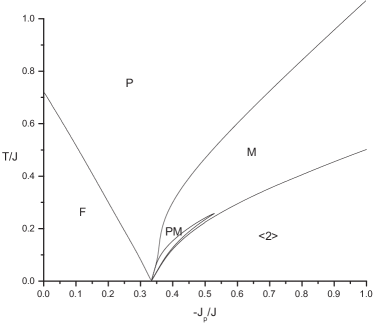
Figure 1: Phase Diagram of the model: $F$ means ferromagnetic, $P$ paramagnetic, $M$ modulated, $PM$ paramodulated, and $<2>$ the antiphase structure, i.e. the structure with period 4.

The Paramagnetic Phase. The transition lines of the para-ferro and para-modulated are found to be continuous. Such lines are obtained by linearizing the system (5) around the fixed point $(x^{*},0,0,0)$. Note that the parameters $y_{1}$, $y_{2}$ and $y_{3}$ vanish in the region $R$. The variable $x^{*}$ is unaffected in first order in $y_{1}$, $y_{2}$ and $y_{3}$.

The eigenvalue equation of the linearized system has the following form:

$$\lambda^{3}+\frac{2(x^{*2}-\theta^{2}_{p}x^{*}-2\theta_{p})}{(\theta+x^{*})[(\theta_{p}+1)x^{*}+2]}\lambda^{2}$$

$$+\frac{4(1-\theta_{p})x^{*}[(\theta_{p}+1)x^{*2}+(\theta_{p}+1)^{2}x^{*}+2]}{(\theta_{p}+x^{*})[(\theta_{p}+1)x^{*}+2]^{2}}\lambda$$

$$+\frac{8(1-\theta_{p})^{2}(\theta_{p}+2)x^{*2}}{(\theta_{p}+x^{*})[(\theta_{p}+1)x^{*}+2]^{2}}=0$$ (8)

The fixed point is linearly stable if the eigenvalues has moduli smaller than one. It is interesting to note that in the Paramagnetic case from (6), one may observe the average magnetization value as being equal to 2.

To find out the transition lines it is necessary to examine several cases with respect to whether the the eigenvalues are real or complex.

The Para-Ferro Transition. When the eigenvalues are real, the transition line will be characterized by the criterion that the largest (in absolute value) eigenvalue should be equal to unity. This determines the stability limit line we were looking for (since all fixed points are linearly stable if the eigenvalues have moduli smaller than one).

The condition that the largest eigenvalue is equal to 1 becomes

$$(6\theta_{p}+2)x^{*3}+(3\theta^{3}_{p}-12\theta^{2}_{p}-7\theta_{p}+28)x^{*2}$$

$$-(4\theta^{2}_{p}+8\theta_{p}-12)x^{*}-4\theta_{p}=0$$ (9)

with $x^{*}$ positive. From this equation one can find $x^{*}$ and taking into account that is a fixed point of (7), one gets an equation of the para-ferro transition line which will be in the form $\theta_{1}=g(\theta_{p})$ for some function $g$.

Note that the case $\theta_{p}=1$ (i.e. $J_{p}=0$) corresponds to the simple Potts model with nearest neighbor interactions and one recovers the well-known result for the critical temperature: $\exp(J/T_{c})=4$ g ; PLM .

Observations of (Phase diagram of the three states Potts model with next nearest neighbor interactions on the Bethe lattice) show that at low temperatures ($\theta_{p}\ll 1$) from (7) one has $x^{*}\sim{\theta_{p}/3}$ and $\theta_{1}\sim{(27/4)\theta^{-3}_{p}}$. In terms of $T$ and $p\equiv-J_{p}/J$, the equation of the transition line is given by

$$1-3p=T\log\bigg{(}\frac{27}{4}\bigg{)}\qquad(T\rightarrow 0),$$

which is in agreement with the slope obtained numerically (see Fig. 1).

The Para-Modulated Transition. When the three eigenvalues are a pair of complex conjugates and one real, then the fixed point is approached in an oscillatory way and stability is achieved if the absolute values of all eigenvalues are less than 1. The critical transition line will then be characterized by the criterion that the modules of the complex eigenvalues are equal to unity. Therefore, the instability occurs when eigenvalue $\lambda=i$. Hence, the eigenvalue equation (Phase diagram of the three states Potts model with next nearest neighbor interactions on the Bethe lattice) is reduced to

$$(5\theta^{2}_{p}+2\theta_{p}-3)x^{*3}+(5\theta^{3}_{p}+6\theta^{2}_{p}+\theta_{p})x^{*2}$$

$$+4(\theta^{2}_{p}+3\theta_{p}-1)x^{*}+4\theta_{p}=0.$$ (10)

If $5\theta^{2}_{p}+2\theta_{p}-3>0$, i.e. $\theta_{p}>\frac{3}{5}$, then equation (2) does not allow for any positive solution. Therefore, the transition exists only if $\theta_{p}<\frac{3}{5}$, that is $\frac{J_{p}}{T}<\log\frac{3}{5}$,

$$-\frac{J_{p}}{J}>\frac{T}{J}\log\frac{5}{3}$$

and it corresponds to the asymptote of the transition line for large $T$ in Fig. 1

Observations of (2) show at low temperatures ($\theta_{p}\ll 1$), $x^{*}\sim{\theta_{p}}$ and from (Phase diagram of the three states Potts model with next nearest neighbor interactions on the Bethe lattice) one finds $\theta_{1}\sim{(1/2)\theta^{-3}_{p}}$. In terms of $T$ and $p\equiv-J_{p}/J$, the equation of the transition line becomes

$$1-3p={-\frac{T}{J}\log 2}\qquad(T\rightarrow 0)$$

which is in agreement with the slope obtained numerically.

The Paramodulated Phase.

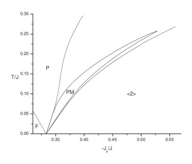
Figure 2: Enlargement of Fig. 1 around the PM phase

As noted earlier that the set $D=\{(x,0,0,0):x\in R_{+}\}$ is invariant for the dynamical system (5), one can consider its restriction to this set, which is given by (7). Numerical investigations of the dynamics of (7) show that in some values of the parameters $T/J_{1}$ and $-J_{p}/J_{1}$ it has 2-periodic points (note that no other periodic points are present). In the plane $(T/J_{1},J_{p}/J_{1})$ such values form an island inside the modulated region (see Fig. 2). In this island, the average magnetization $m$ is equal to 2 as in the paramagnetic case. Therefore, we denote it as paramodulated (PM) phase. A similar phase is not present in the case of the Ising model, hence marking a difference between Potts and Ising models V ; MTA . In Fig. 3 and Fig. 4 plots of the values of magnetization $m$ are given at selected values $-J_{p}/J=0.36$ and $-J_{p}/J=0.56$, respectively. Note that this phase also issues from the multi-critical point (the Lifshitz point) $T=0,-J_{p}/J_{1}=1/3$.

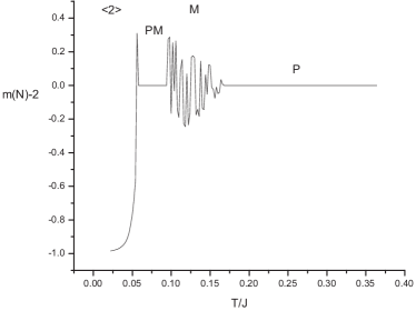
Figure 3: The average magnetization versus $T/J$ for $-J_{p}/J=0.36$.

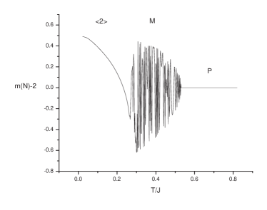
Figure 4: The average magnetization versus $T/J$ for $-J_{p}/J=0.56$.

Discussions. We have found an exact phase diagram of the Potts model with next nearest neighbor interactions on the Bethe lattice of order two. The diagram consists of five phases: ferromagnetic, paramagnetic, modulated, antiphase and paramodulated, all meeting at the Lifshift point i.e. $p=1/3$. A distinctive feature of the diagram is seen in the existence of a new phase called the paramodulated phase found at low temperatures and characterized by 2-periodic points of the dynamical system (7). This phase lies inside the modulated phase and is inherent in the Potts model as no analogue can be found within the Ising setting. We believe the appearance of such a phase to essentially be another form of symmetry resulting in the increasing of the number of spin from two to three.

- (1) M.P. Nightingale, M. Schick, J.Phys. A: Math. Gen. 15, L39-L42 (1982).
- (2) R.J. Baxter, Exactly Solved Models in Statistical Mechanics, (Academic Press, London/New York, 1982).
- (3) S.N. Dorogovtsev, A.V. Goltsev, J.F.F.Mendes, Eur. Phys. J. B 38 177-182 (2004).
- (4) J.L. Monroe, Physics Lett. A. 188, 80-84 (1994); Phys. Rev. E 67 , 017103 (2003).
- (5) P.N. Timonin, JETP 99 , 1044–1053 (2004).
- (6) R.B. Potts, Proc. Cambridge Philos. Soc. 48, 106–109 (1952).
- (7) F.Y. Wu, Rev. Mod. Phys. 54 , 235–268 (1982).
- (8) S. Coutinho, W. A. M. Morgado, E. M. F. Curado, L. da Silva, Phys. Rev. 74, 094432 (2006)
- (9) F. Peruggi, F. di Liberto, G. Monroy, J. Phys. A 16 , 811–827 (1983); Physica A 141 151–186 (1987).
- (10) N.N. Ganikhodjaev, Theor. Math. Phys. 85 , 1125–1134 (1990).
- (11) The Ising model with competing interactions was originally considered by Elliot E in order to describe modulated structures in rare-earth systems. In BB the interest to the model was renewed and studied by means of an iteration procedure. The Ising type models on the Bethe lattices with competing interactions appeared in a pioneering work Vannimenus V , in which the physical motivations for the urgency of the study such models were presented. In YOS ; TY the infinite-coordination limit of the model introduced by Vannimenus was considered. It was also found a phase diagram which was similar to that model studied in BB . In MTA ,SC other generalizations of the model were studied.
- (12) R.J. Elliott, Phys. Rev., 124, 340–345 (1961).
- (13) P.Bak, J.von Boehm, Phys. Rev. B,21, 5297–5308 (1980).
- (14) J.Vannimenus, Z.Phys. B 43, 141–148 (1981).
- (15) C.S.O.Yokoi, M.J. Oliveira, S.R. Salinas, Phys. Rev. Lett., 54, 163–166 (1985).
- (16) M.H.R. Tragtenberg, C.S.O. Yokoi, Phys. Rev. B, 52, 2187–2197 (1995).
- (17) M. Mariz, C.Tsalis, A.L.Albuquerque, Jour. Stat. Phys. 40, 577–592 (1985).
- (18) C.R. da Silca, S. Coutinho, Phys. Rev. B,34, 7975-7985 (1986).
- (19) F.A. Kassan-Ogly, B.N. Filippov, Jour. Magnetism. Magn. Mat. 300, 559–562 (2006); F.A. Kassan-Ogly, I.V. Sagaradze, Phys. Metals Metallography 100 201-207 (2005).
- (20) I. Peschel, T. T. Truong, Jour. Stat. Phys. 45 1572–9613 (1986).
- (21) M.C. Marques, J.Phys. A: Math. Gen. 21, 1061-1068 (1988).
- (22) M. Tarnawski J. Phys.: Condens. Matter 1, 1849-1854 (1989); 2 8599–8613 (1990).
- (23) J.R. Banavar, F.Y Wu, Physical Review B 29 1511-1513 (1984)
- (24) M. Itakura, Phys. Rev. B 55, 48 - 51 (1997).
- (25) One dimensional Potts models with next nearest neighbor interactions were studied in KF ,CS . Recently, in gmm the Potts model with one level competing intercations on a Bethe lattice has been exactly solved.
- (26) S.-C. Chang, R. Shrock, Inter. J. Mod. Phys. B 15 443-478 (2001). R. Shrock, S.-H. Tsai, Phys. Rev. E 55 5184-5193 (1997).
- (27) N.N. Ganikhodjaev, F.M. Mukhamedov, J.F.F. Mendes, Jour. Stat. Mech. P08012 (2006).
- (28) S. Aubry, in Solutions and Condesend Matter, edited by A.R. Bishop and T.Schneider (Springer-Verlag, Berlin, 1978).