Logical Queries over Views: Decidability and Expressiveness

Abstract

We study the problem of deciding satisfiability of first order logic queries over views, our aim being to delimit the boundary between the decidable and the undecidable fragments of this language. Views currently occupy a central place in database research, due to their role in applications such as information integration and data warehousing. Our main result is the identification of a decidable class of first order queries over unary conjunctive views that generalises the decidability of the classical class of first order sentences over unary relations, known as the Löwenheim class. We then demonstrate how various extensions of this class lead to undecidability and also provide some expressivity results. Besides its theoretical interest, our new decidable class is potentially interesting for use in applications such as deciding implication of complex dependencies, analysis of a restricted class of active database rules, and ontology reasoning.

1 Introduction

The study of views in relational databases has attracted much attention over the years. Views are an indispensable component for activities such as data integration and data warehousing [Widom (1995), Garcia-Molina et al. (1995), Levy et al. (1996)], where they can be used as “mediators” for source information that is not directly accessible to users. This is especially helpful in modelling the integration of data from diverse sources, such as legacy systems and/or the world wide web.

Much of the research related to views has addressed fundamental problems such as containment and rewriting/optimisation of queries using views (e.g. see [Ullman (1997), Halevy (2001)]). In this paper, we examine the use of views in a somewhat different context, where they are used as the basic unit for writing logical expressions. We provide results on the related decision problem in this paper, for a range of possible view definitions. In particular, for the case where views are monadic/unary conjunctive queries, we show that the corresponding query logic is decidable. This corresponds to an interesting new fragment of first order logic. On the application side, this decidable query language also has some interesting potential applications for areas such as implication of complex dependencies, ontology reasoning and termination results for active rules.

1.1 Informal Statement of the Problem

Consider a relational vocabulary $R_{1},\ldots,R_{p}$ and a set of views $V_{1},\ldots,V_{n}$. Each view definition corresponds to a first order formula over the vocabulary. Some example views (using horn clause style notation) are

$V_{1}(x_{1},y_{1})\leftarrow R_{1}(x_{1},y_{1}),R_{2}(y_{1},y_{1},z_{1}),R_{3}(z_{1},z_{2},x_{1}),R_{4}(z_{2},x_{1})$

$V_{2}(z_{1})\leftarrow R_{1}(z_{1},z_{1})$

Each such view can be expanded into to a first order sentence, e.g. $V_{1}(x_{1},y_{1})\Leftrightarrow\exists z_{1},z_{2}(R_{1}(x_{1},y_{1})\wedge R_{2}(y_{1},y_{1},z_{1}),R_{3}(z_{1},z_{2},x_{1})\wedge\neg R_{4}(z_{2},x_{1}))$. A first order view query is a first order formula expressed solely in terms of the given views. e.g. $q_{1}=\exists x_{1},y_{1}((V_{1}(x_{1},y_{1})\vee V_{1}(y_{1},x_{1}))\wedge\neg V_{2}(x_{1}))\wedge\forall z_{1}(V_{2}(z_{1})\Rightarrow V_{1}(z_{1},z_{1}))$ is an example first order view query, but $q_{2}=\exists x_{1},y_{1}(V_{1}(x_{1},y_{1})\vee R(y_{1},x_{1}))$ is not. By expanding the view definitions, every first order view query can clearly be re-written to eliminate the views. Hence, first order view queries can be thought of as a fragment of first order logic, with the exact nature of the fragment varying according to how expressive the views are permitted to be.

From a database perspective, first order view queries are particularly suited to applications where the source data is unavailable, but summary data (in the form of views) is. Since many database and reasoning languages are based on first order logic (or extensions thereof), this makes it a useful choice for manipulating the views.

Our purpose in this paper is to determine, for what types of view definitions, satisfiability (over both finite and infinite models) is decidable for the language. If views can be binary, then this language is clearly as powerful as first order logic over binary base relations, and hence undecidable (see [Boerger et al. (1996)]). The situation becomes far more interesting, when we restrict the form that views may take — in particular, when their arity must be unary. Such a restriction has the effect of constraining which parts of the underlying database can be “seen” by the view formula and also constrains how such parts may be connected.

1.2 Contributions

The main contribution of this paper is the definition of a language called the first order unary conjunctive view language (UCV) and a proof of its decidability. As its name suggests, it uses unary arity views defined by conjunctive queries. We demonstrate that it is a maximal decidable class, in the sense that increasing the expressiveness of the view definitions results in undecidability. Some interesting aspects of this decidability result are:

• It is well known that first order logic solely over monadic relations is decidable [Löwenheim (1915)], but the extension to dyadic relations is undecidable [Börger et al. (1997)]. The first order unary conjunctive view language can be seen as an interesting intermediate case between the two, since although only monadic predicates (views) appear in the query, they are intimately related to database relations of higher arity.

• The language is able to express some interesting properties, which might be applied to various kinds of reasoning over ontologies. It can also be thought of as a powerful generalisation of unary inclusion dependencies [Cosmadakis et al. (1990)]. Furthermore, it has an interesting characterisation as a decidable class of rules (triggers) for active databases.

To briefly give a feel for this decidable language, we next provide some example unary conjunctive views and a first order unary conjunctive view query defined over them:

$V_{1}(x)\leftarrow R_{1}(x,y),R_{2}(y,z),R_{3}(z,x^{\prime}),R_{4}(x^{\prime},x)$

$V_{2}(x)\leftarrow R_{1}(x,y),R_{1}(x,z),R_{4}(y,z)$

$V_{3}(x)\leftarrow R_{1}(x,y),R_{1}(x,z),R_{4}(y,y),R_{4}(z,x)$

$V_{4}(x)\leftarrow R_{1}(x,y),R_{3}(y,z),R_{4}(z,x^{\prime}),R_{4}(x^{\prime},y^{\prime}),R_{3}(y^{\prime},x)$

$\exists x(V_{2}(x)\wedge\neg V_{1}(x))\wedge\neg\exists y(V_{3}(y)\wedge\neg V_{4}(y))$

1.3 Paper Outline

The paper is structured as follows: Section 2 defines the necessary preliminaries and background concepts. Section 3 presents the definition of the logic UCV. Section 4 is the core section of the paper, where the decidability result for the class UCV is proved. Section 5 shows that extensions to the language, such as allowing negation, inequality or recursion in views, result in undecidability. Section 6 covers applications of the decidability results and then Section 7 provides some results on expressivity. Section 8 discusses related work and section 9 summarises and discusses future work.

2 Preliminaries

In this section, we state basic definitions and relevant results. The reader is assumed to be familiar with standard results and notations from mathematical logic (e.g. see [Enderton (2001)]). In the following, formulas are always first-order. The symbol $\mathcal{FO}$ denotes the set of first order formulas over any vocabulary $\sigma$. In addition, if $\mathcal{L}\subseteq\mathcal{FO}$ (i.e. $\mathcal{L}$ is a fragment of $\mathcal{FO}$), we denote by $\mathcal{L}(\sigma)$ the set of formulas in $\mathcal{L}$ over the vocabulary $\sigma$.

2.1 First-order logic

A (relational) vocabulary $\sigma$ is a tuple $\langle R_{1},\ldots,R_{n}\rangle$ of relation symbols with each $R_{i}$ associated with a specified arity $r_{i}$. A (relational) $\sigma$-structure A is the tuple

$$\langle A;R_{1}^{\mbox{{{A}}}},\ldots,R_{n}^{\mbox{{{A}}}}\rangle$$

where $A$ is a non-empty set, called the universe (of A), and $R_{i}^{\mbox{{{A}}}}$ is an $r_{i}$-ary relation over $A$ interpreting $R_{i}$. We refer to the elements in the set $A$ as the elements in A, or simply by constants (of A). In the sequel, we write $R_{i}$ instead of $R_{i}^{\mbox{{{A}}}}$ when the meaning is clear from the context. We also use $STRUCT(\sigma)$ to denote the set of all $\sigma$-structures. We assume a countably infinite set VAR of variables. An instantiation (or valuation) of a structure I is a function $v:\text{VAR}\rightarrow I$. Extend this function to free tuples (i.e. tuple of variables) in the obvious way. We use the usual Tarskian notion of satisfaction to define $\mbox{{I}}\models\phi[v]$, i.e., whether $\phi$ is true in I under $v$. If $\phi$ is a sentence, we simply write $\mbox{{I}}\models\phi$. The image of a structure I under a formula $\phi(x_{1},\ldots,x_{n})$ is

$$\phi(\mbox{{I}})\overset{\mbox{\tiny def}}{=}\{v(x_{1},\ldots,x_{n}):\text{$v$ is an instantiation of $\mbox{{I}}$, and $\mbox{{I}}\models\phi[v]$}\}.$$

In particular, if $n=0$, we have that $\phi(\mbox{{I}})\neq\emptyset$ iff $\mbox{{I}}\models\phi$. We say that two $\sigma$-structures A and B agree on ${\cal L}$ iff for all $\phi\in{\cal L}(\sigma)$ we have $\mbox{{{A}}}\models\phi\Leftrightarrow\mbox{{{B}}}\models\phi$.

Following the convention in database theory, the (tuple) database $\mathcal{D}(\mbox{{{A}}})$ corresponding to the structure A (defined above) is the set

$$\{R_{i}(t):\text{$1\leq i\leq n$ and $t\in R_{i}^{\mbox{{{A}}}}$}\}.$$

It is easy to see that such a database can be considered a structure with universe $adom(\mbox{{{A}}})$, which is defined to be the set of all elements of A occurring in at least one relation $R_{i}$, and relations built appropriately from $\mathcal{D}(\mbox{{{A}}})$. Abusing terminologies, we refer to the elements of $\mathcal{D}(\mbox{{{A}}})$ as tuples (associated with A). In addition, when the meaning is clear from the context, we shall also abuse the term free tuple to mean an atomic formula $R(u)$, where $R\in\sigma$ and $u$ is a tuple of variables.

A formula $\phi$ is said to be satisfiable if there exists a structure A (either of finite or infinite size) such that $\phi(\mbox{{{A}}})\neq\emptyset$; such a structure is said to be a model for $\phi$. We say that $\phi$ is finitely satisfiable if there exists a finite structure I such that $\phi(\mbox{{I}})\neq\emptyset$. Without loss of generality, we shall focus only on sentences when we are dealing with the satisfiability problem. In fact, if $\phi$ has some free variables, taking its existential closure preserves satisfiability [Indeed we shall see that the languages we consider are closed under first-order quantification].

Given two $\sigma$-structures $\mbox{{{A}}},\mbox{{{B}}}$, recall that A is a substructure of B (written $\mbox{{{A}}}\subseteq\mbox{{{B}}}$) if $A\subseteq B$ and $R^{\mbox{{{A}}}}\subseteq R^{\mbox{{{B}}}}$ for every relation symbol $R$ in $\sigma$. We say that A is an induced substructure of B (i.e. induced by $A\subseteq B$) if for every relation symbol $R$ in $\sigma$, $R^{\mbox{{{A}}}}=R^{\mbox{{{B}}}}\cap A^{r}$, where $r$ is the arity of $R$. Now, a homomorphism from A to B is a function $h:A\rightarrow B$ such that, for every relation symbol $R$ in $\sigma$ and $\mbox{{{a}}}=(a_{1},\ldots,a_{r})\in R^{\mbox{{{A}}}}$, it is the case that $h(\mbox{{{a}}})\overset{\mbox{\tiny def}}{=}(h(a_{1}),\ldots,h(a_{r}))\in R^{\mbox{{{B}}}}$. An isomorphism is a bijective homomorphism whose inverse is a homomorphism.

The quantifier rank $\mbox{qrank}(\phi)$ of of a formula $\phi$ is the maximum nesting depth of quantifiers in $\phi$.

2.2 Views

For our purpose, a view over $\sigma$ can be thought of as an arbitrary FO formula over $\sigma$. We say that a view $V$ is conjunctive if it can be written as a conjunctive query, i.e. of the form

$$\exists x_{1},\ldots,x_{n}(R_{1}(u_{1})\wedge\ldots\wedge R_{k}(u_{k}))$$

where each $R_{i}$ is a relation symbol, and each $u_{i}$ is a free tuple of appropriate arity. We adopt the horn clause style notation for writing conjunctive views. For example, if $\{y_{1},\ldots,y_{n}\}$ is the set of free variables in the above conjunctive query, then we can rewrite it as

$$V(y_{1},\ldots,y_{n})\leftarrow R_{1}(u_{1}),\ldots,R_{k}(u_{k})$$

where $V(y_{1},\ldots,y_{n})$ is called the head of $V$, and the conjunction $R_{1}(u_{1}),\ldots,R_{k}(u_{k})$ the body of $V$. The length of the conjunctive view $V$ is defined to be the sum of the arities of the relation symbols in the multiset $\{R_{1},\ldots,R_{k}\}$. For example, the lengths of the two views $V$ and $V^{\prime}$ defined as

$$V(x) \leftarrow E(x,y)$$

$$V^{\prime}(x) \leftarrow E(x,y),E(y,z)$$

are, respectively, two and four. Additionally, if $n=1$ (i.e. has a head of arity 1), the view is said to be unary. Unless stated otherwise, we shall say “view” to mean “unary-conjunctive view with neither equality nor negation in its body”.

2.3 Graphs

We use standard definitions from graph theory (e.g. see [Diestel (2005)]). A graph is a structure $\mbox{{{G}}}=(G,E)$ where $E$ is a binary relation. The girth of a graph is the length of its shortest cycle. For two vertices $x,y\in G$, we denote their distance by $d_{\mbox{{{G}}}}(x,y)$ (or just $d(x,y)$ when G is clear from the context). For two sets $S_{1}$ and $S_{2}$ of vertices in G, we define their distance to be

$$d_{\mbox{{{G}}}}(S_{1},S_{2}):=\min\{d_{\mbox{{{G}}}}(a,b):\text{$a\in S_{1}$ and $b\in S_{2}$}\}.$$

In a weighted graph G with weight $w_{\mbox{{{G}}}}:E\rightarrow\mathbb{N}$, the weight $w_{\mbox{{{G}}}}(P)$ of a path $P$ in G is just $\sum_{e\in E(P)}w_{\mbox{{{G}}}}(e)$. We shall write $w$ instead of $w_{\mbox{{{G}}}}$ if the meaning is clear from the context. In the sequel, we shall frequently mention trees and forests. We always assume that any tree has a selected node, which we call a root of the tree. Given a tree $\mbox{{{T}}}=(T,E)$, we can partition $T$ according to the distance of the vertices from the root.

The Gaifman graph (see [Gaifman (1982)]) associated with a structure A is the weighted undirected multi-graph $\mathbb{G}(\mbox{{{A}}})=(G,E)$ such that:

1. $G=A$.

2. The multi-set $E$ is defined as follows: for each $x,y\in G$, we put an $R(t)$-labeled edge $xy$ in $E$ with weight $r$ (the arity of $R$) iff $x$ and $y$ appear in a tuple $R(t)$ in $\mathcal{D}(\mbox{{{A}}})$. [Notice that the multiplicity of $xy$ in $E$ depends on the number of tuples in $\mathcal{D}(\mbox{{{A}}})$ that contain both $x$ and $y$ as their arguments.]

Note also that the subgraph of $\mathbb{G}(\mbox{{{A}}})$ induced by the set of all elements of A in a tuple $t$ is the complete graph $K_{r}$, and so an $L$-labelled edge is adjacent to an edge $e\in E$ iff all $L$-labelled edges are adjacent (i.e. connected) to the edge $e$. For any $a,b\in A$, we define the distance $d_{\mbox{{{A}}}}(a,b)$ between $a$ and $b$ to be their distance in $\mathbb{G}(\mbox{{{A}}})$. Also, extend this distance function to tuples and sets of tuples by interpreting them as sets of elements of A that appear in them. Any pair of tuples $R(t)$ and $R^{\prime}(t^{\prime})$ in $\mathcal{D}(\mbox{{{A}}})$ are said to be connected (in A) if in $\mathbb{G}(\mbox{{{A}}})$ some (and hence all) $R(t)$-labeled edge is adjacent to some (and hence all) $R^{\prime}(t^{\prime})$-labeled edge.

2.4 Unary formulas

A unary formula is an arbitrary FO formula without equality such that each of its relation symbols has arity one. Let $\sigma$ be a vocabulary whose relation symbols are of arity one. We shall use $\text{UFO}(\sigma)$ to denote the set of all unary formulas without equality over $\sigma$. Also, we define $\text{UFO}=\cup_{\sigma}\text{UFO}(\sigma)$. The following lemma will be useful for proving expressiveness results in Section 7.

Lemma 2.1

For every unary sentence, there exists an equivalent one of quantifier rank 1.

Proof.

By a straightforward manipulation. See the proof of lemma 21.12 in [Boolos et al. (2002)]. [Their proof actually gives more than the result they claim. In fact, their construction converts an arbitrary unary sentence into one with one unary variable and of quantifier rank 1.] ∎

2.5 Ehrenfeucht-Fraïsse Games

We shall need a limited form of Ehrenfeucht-Fraïsse games; for a general account, the reader may consult [Libkin (2004)]. The games are played by two players, Spoiler and Duplicator, on two $\sigma$-structures A and B. The goal of Spoiler is to show that the structures are different, while Duplicator aims to show that they are the same. The game consists of a single round. Spoiler chooses a structure (say, A) and an element $a$ in it, after which Duplicator has to respond by choosing an element $b$ in the other structure B. Duplicator wins the game iff the substructure of A induced by $\{a\}$ is isomorphic to the substructure of B induced by $\{b\}$. Duplicator has a winning strategy iff Duplicator has a winning move, regardless of how Spoiler behaves.

Proposition 2.2 ((Ehrenfeucht-Fraïsse Games))

Duplicator has a winning strategy on A and B iff A and B agree on first-order formulas over $\sigma$ of quantifier rank 1.

2.6 Other Notation

Regarding other notation we shall use throughout the rest of the paper: we shall use $a,b$ for constants, $x,y,z$ for variables, $u$ for free tuples, $U,V$ for views, $\mathcal{U},\mathcal{V}$ for sets of views, $\sigma$ for vocabularies, $R_{1},R_{2},\ldots$ for relation symbols, $\mbox{{{A}}},\mbox{{{B}}},\ldots$ for structures and $A,B$ for their respective universes. If $\mathcal{D}$ is a database (a set of tuples), we use $adom(\mathcal{D})$ to denote the set of constants in $\mathcal{D}$. Finally, given a $a\in adom(\mathcal{D})$ and a “new” constant $b\notin\mathcal{D}$, we define $\mathcal{D}[b/a]$ to be the database that is obtained from $\mathcal{D}$ by replacing every occurrence of $a$ by $b$. The notation $\mathcal{D}[b_{1}/a_{1},\ldots,b_{n}/a_{n}]$ is defined in the same way.

3 Definition of First Order Unary-conjunctive-view Logic

Let $\sigma$ be an arbitrary vocabulary, and $\mathcal{V}$ be a finite set of (unary conjunctive) views over $\sigma$, which we refer to as a $\sigma$-view set. We now inductively define the set $\text{UCV}(\sigma,\mathcal{V})$ of first order unary-conjunctive-view (UCV) queries/formulas over the vocabulary $\sigma$ and a $\sigma$-view set $\mathcal{V}$:

1. if $V\in\mathcal{V}$, then $V(x)\in\text{UCV}(\sigma,\mathcal{V})$; and

2. if $\phi,\psi\in\text{UCV}(\sigma,\mathcal{V})$, then the formulas $\neg\phi,\phi\wedge\psi$ and $\exists x\phi$ belong to $\text{UCV}(\sigma,\mathcal{V})$.

The smallest set of so-constructed formulas defines the set $\text{UCV}(\sigma,\mathcal{V})$. We denote the set of all UCV formulas over the vocabulary $\sigma$ by $\text{UCV}(\sigma)$, i.e. $\text{UCV}(\sigma)\overset{\mbox{\tiny def}}{=}\bigcup_{\mathcal{V}}\text{UCV}(\sigma,\mathcal{V})$ where $\mathcal{V}$ may be any $\sigma$-view set. Further, the set of all UCV queries is denoted by UCV, i.e. $\text{UCV}\overset{\mbox{\tiny def}}{=}\bigcup_{\sigma}\text{UCV}(\sigma)$, where $\sigma$ is any vocabulary. As usual, we use the shorthands $\phi\vee\psi$, $\phi\rightarrow\psi$, $\phi\leftrightarrow\psi$, and $\forall x\phi$ for (respectively) $\neg(\neg\phi\wedge\neg\psi),\neg\phi\vee\psi,(\phi\rightarrow\psi)\wedge(\psi\rightarrow\phi)$, and $\neg\exists x\neg\phi$. Thus, the UCV language is closed under boolean combinations and first-order quantifications. As an example, consider the UCV formula

$$q_{1}=\exists x(V(x)\wedge\neg V^{\prime}(x))$$

where $V$ and $V^{\prime}$ are defined as

$$V(x) \leftarrow E(x,y)$$

$$V^{\prime}(x) \leftarrow E(x,y),E(y,z)$$

This formula asserts that there exists a vertex from which there is an outgoing arc, but no outgoing directed walk of length 2.

Let us make a few remarks on the expressive power of the logic UCV with respect to other logics. It is easy to see that the UCV language strictly subsumes UFO  (the Löwenheim class without equality [Löwenheim (1915), Börger et al. (1997)]), as UCV queries can be defined over any relational vocabularies (i.e. including ones that include $k$-ary relation symbols with $k>1$). It is also easy to see that allowing any general existential positive formula (i.e. of the form $\exists\overline{x}\phi(\overline{x})$ where $\phi$ is a quantifier-free formula with no negation) with one free variable, does not increase the expressive power of the logic. Indeed, the quantifier-free subformula $\phi$ can be rewritten in disjunctive normal form without introducing negation, after which we may distribute the existential quantifier across the disjunctions and consequently transform entire formula to a disjunction of conjunctive queries with one or zero free variables. Each such conjunctive query can then be treated as a view.

There are two ways in which we can interpret a UCV formula. The standard way is to think of a UCV query as an FO formula over the underlying vocabulary. Take the afore-mentioned query $q_{2}$ as an example. We can interpret this query as the formula

$$\exists x(\exists y,z(E(x,y)\wedge E(y,z))\wedge\neg\exists y(E(x,y))$$

over the graph vocabulary. The non-standard way is to regard a UCV query $\phi$ as a unary formula over the view set. For example, we can think of $q_{2}$ as a unary formula over the vocabulary $\sigma^{\prime}=\langle V,V^{\prime}\rangle$. Now, if $\phi\in\text{UCV}(\sigma,\mathcal{V})$, then we denote by $\phi^{\mathcal{V}}$ the unary formula over $\mathcal{V}$ corresponding to $\phi$ in the non-standard interpretation of UCV queries. However, for notational convenience, we shall write $\phi$ instead of $\phi^{\mathcal{V}}$ when the meaning is clear from the context. Given a vocabulary $\sigma$ and a $\sigma$-view set $\mathcal{V}=\{V_{1},\ldots,V_{n}\}$, we may define the function $\Lambda:STRUCT(\sigma)\rightarrow STRUCT(\mathcal{V})$ such that for any $\mbox{{I}}\in STRUCT(\sigma)$

$$\Lambda(\mbox{{I}})\overset{\mbox{\tiny def}}{=}\langle I;V_{1}^{\Lambda(\mbox{{I}})},\ldots,V_{n}^{\Lambda(\mbox{{I}})}\rangle$$

where $V_{i}^{\Lambda(\mbox{{I}})}\overset{\mbox{\tiny def}}{=}V_{i}(\mbox{{I}})$. For example, let $\sigma=\langle E\rangle$ and $\mathcal{V}=\{V,V^{\prime}\}$ be as above, and let

$$\mbox{{I}}=\langle\{1,2,3,4\};E^{\mbox{{I}}}=\{(1,2),(2,3),(3,4)\}\rangle.$$

Then, we have

$$\mbox{{J}}\overset{\mbox{\tiny def}}{=}\Lambda(\mbox{{I}})=\langle\{1,2,3,4\},V^{\mbox{{J}}}=\{1,2,3\},V^{\prime\mbox{{J}}}=\{1,2\}\rangle.$$

In the following, we shall reserve the symbol $\Lambda$ to denote this special function. In addition, if $\mbox{{J}}\in STRUCT(\mathcal{V})$ and there exists a structure $\mbox{{I}}\in STRUCT(\sigma)$ such that $\Lambda(\mbox{{I}})=\mbox{{J}}$, we say that the structure J is realizable with respect to the vocabulary $\sigma$ and the view set $\mathcal{V}$, or that I realizes J. We shall omit mention of $\sigma$ and $\mathcal{V}$ if they are understood by context.

A number of remarks about the notion of realizability are in order. First, some unary structures are not realizable with respect to a given view set $\mathcal{V}$. For example, the query $q_{2}$ has infinitely many models if treated as a unary formula, but none of these models are realizable, since $V^{\prime}\subseteq V$. Second, if $\phi\in\text{UCV}(\sigma,\mathcal{V})$ has a model I, then the structure $\Lambda(\mbox{{I}})$ over $\mathcal{V}$ is a model for $\phi^{\mathcal{V}}$. In other words, if a UCV query is satisfiable, then it is also satisfiable if treated as a unary formula. Conversely, it is also clearly true that a UCV query is satisfiable, if it is satisfiable when treated as a unary formula and that at least one of its models is realizable. More precisely, if $\Lambda(\mbox{{I}})$ is a model for $\phi^{\mathcal{V}}$, then I is a model for $\phi$. So, combining these, we have $I\models\phi$ iff $\Lambda(I)\models\phi^{\mathcal{V}}$. So, we immediately have the following lemma:

Lemma 3.1

Suppose $\mbox{{{A}}},\mbox{{{B}}}\in STRUCT(\sigma)$ and $\phi\in\text{UCV}(\sigma,\mathcal{V})$. Then, for $\Lambda:STRUCT(\sigma)\rightarrow STRUCT(\mathcal{V})$ defined above, the following statements are equivalent:

1. $\mbox{{{A}}}\models\phi$ iff $\mbox{{{B}}}\models\phi$,

2. $\Lambda(\mbox{{{A}}})\models\phi^{\Lambda}$ iff $\Lambda(\mbox{{{B}}})\models\phi^{\Lambda}$.

This lemma is useful when combined with Ehrenfeucht-Fraïsse games. For example, suppose that we are given a model A for $\phi$, and we construct a “nicer” structure B that, we wish, satisfies $\phi$. If we can prove that the second statement in the lemma (which is often easier to establish as views have arity one), we might deduce that $\mbox{{{B}}}\models\phi$.

4 Decidability of UCV Queries

In this section, we prove our main result that satisfiability is decidable for UCV formulas. Our main theorem stipulates that UCV has the bounded model property.

Theorem 4.1

Let $\phi$ be a formula in UCV. Suppose, further, that $\phi$ contains precisely the views in the view set $\mathcal{V}$, and relation symbols in the vocabulary $\sigma$, with $m$ being the maximum length of the views in $\mathcal{V}$, and $p=|\sigma|$. If $\phi$ is satisfiable, then it has a model using at most $2^{2^{q(p,m)}}$ elements, for some fixed polynomial $q$ in $p$ and $m$.

Before we prove this theorem, we first derive some corollaries. Simple algebraic manipulations yield the following corollary.

Corollary 4.2

Continuing from Theorem 4.1, if $n$ is the size of (the parse tree of) a satisfiable formula $\phi$, then $\phi$ has a model of size $2^{2^{g(n)}}$ for some fixed polynomial $g$ in $n$.

Corollary 4.2 immediately leads to the decidability of satisfiability for UCV. We can in fact derive a tighter bound.

Theorem 4.3

Satisfiability for the UCV class of formulas is in 2-NEXPTIME.

This theorem follows immediately from the following proposition and corollary 4.2.

Proposition 4.4

Let $s$ be a non-decreasing function with $s(n)\geq n$. Then, the problem of determining whether an FO sentence has a model of size at most $s(n)$, where $n$ is the size of the input formula, can be decided nondeterministically in $2^{O(n\log(s(n)))}$ steps.

Proof.

We may use any reasonable encoding $\text{code}(\mbox{{{A}}})$ of a finite structure A in bits (e.g. see [Libkin (2004), Chapter 6]). The size of the encoding, denoted $|\mbox{{{A}}}|$, is polynomial in $|A|$. We first guess a structure A of size at most $s(n)$. Let $s^{\prime}=|A|$. Since the size $|\mbox{{{A}}}|$ of the encoding of A is polynomial in $s^{\prime}$, the guessing procedure takes $O(s^{k}(n))$ time steps for some constant $k$. We, then, use the usual procedure for evaluating whether $\mbox{{{A}}}\models\phi$. This can be done in $O(n\times|\mbox{{{A}}}|^{n})$ steps (e.g. see [Libkin (2004), Proposition 6.6]). Simple algebraic manipulations give the sought after upper bound. ∎

Observe that a lower bound for satisfiability of UCV formulas follows immediately from the NEXPTIME completeness for satisfiability of UFO  formulas given in [Börger et al. (1997)]

Theorem 4.5

Satisfiability for the UCV class of formulas is NEXPTIME hard.

What remains now is to prove theorem 4.1.

of theorem 4.1.

Let $\phi,m,p$ be as stated in theorem 4.1. We begin by first enumerating all possible views over $\sigma$ of length at most $m$. As we shall see later in the proof of Subproperty 4.14, doing so will help facilitate the correctness of our construction of a finite model, since enumerating all such views effectively allows us to determine all possible ways the model may be “seen” by views, or parts of views. Let $\mathcal{U}=\{V_{1},\ldots,V_{N}\}$ be the set of all non-equivalent views obtained. By elementary counting, one may easily verify that $N\leq m(mp)^{m}$. Indeed, each view is composed of its head and its body, whose length is bounded by $m$. The body is a set of conjuncts that we may fix in some order. There are at most $m$ variables that the head can take. Each position in the body is a variable ($m$ choices) that is part of a relation $R$ ($p$ choices). The upper bound is then immediate.

Let $\mbox{{I}}_{0}$ be a (possibly infinite) model for $\phi$. [If it is infinite, by the Löwenheim-Skolem theorem, we may assume that it is countable.] Without loss of generality, we may assume that there exists a “universe” relation $U$ in $\mbox{{I}}_{0}$ which contains each constant in $adom(\mbox{{I}}_{0})$. Otherwise, if $U^{\prime}\notin\sigma$ is a unary relation symbol, the $(\sigma\cup\{U^{\prime}\})$-structure obtained by adding to $\mbox{{I}}_{0}$ the relation $U^{\prime}$, which is to be interpreted as $I_{0}$, is also a model for $\phi$.

Let us now define $2^{N}$ formulas $C_{0},\ldots,C_{2^{N}-1}$ of the form

$$C_{i}(x)\overset{\mbox{\tiny def}}{=}(\neg)V_{1}(x)\wedge\ldots\wedge(\neg)V_{N}(x),$$

where the conjunct $V_{j}(x)$ is negated iff the $j$th bit of the binary representation of $i$ is 0. For each $\mbox{{{A}}}\in STRUCT(\sigma)$, these formulas induce an equivalence relation on $A$ with each set $C_{i}(\mbox{{{A}}})$ being an equivalence class. When A is clear, we refer to the equivalence class $C_{i}(\mbox{{{A}}})$ simply as $C_{i}$. In addition, the existence of the universe relation $U$ in $\mbox{{I}}_{0}$ implies that the all-negative equivalence class $C_{0}$ is empty.

We next describe a sequence of five satisfaction-preserving procedures for deriving a finite model from $\mbox{{I}}_{0}$. This sequence is best described diagrammatically:

$$\mbox{{I}}_{0}\stackrel{{\scriptstyle\text{\tt makeJF}}}{{\longrightarrow}}\mbox{{I}}_{1}\stackrel{{\scriptstyle\text{\tt rename1}}}{{\longrightarrow}}\mbox{{I}}_{2}\stackrel{{\scriptstyle\text{\tt rename2}}}{{\longrightarrow}}\mbox{{I}}_{3}\stackrel{{\scriptstyle\text{\tt copy}}}{{\longrightarrow}}\mbox{{I}}_{4}\stackrel{{\scriptstyle\text{\tt prune}}}{{\longrightarrow}}\mbox{{I}}_{5}.$$

The $i$th procedure above takes a structure $\mbox{{I}}_{i}$ as input, and outputs another structure $\mbox{{I}}_{i+1}$. The structure $\mbox{{I}}_{5}$ is guaranteed to be finite (and indeed bounded). That each procedure preserves satisfiability immediately follows by subproperties 4.8, 4.10, 4.12, 4.13, and 4.14. While reading the description of the procedures below, it is instructive to keep in mind that the property that $C_{i}(\mbox{{I}}_{j})=\emptyset$ iff $C_{i}(\mbox{{I}}_{j+1})=\emptyset$ is sufficient for showing that the $j$th procedure preserves satisfiability (see lemma 4.7).

Roughly speaking, the procedure makeJF transforms the initially given structure $\mbox{{I}}_{0}$ into another structure that has a forest-like graphical representation, called a “justification forest”. Each subsequent procedure works only on justification forests. In the sequel, we shall use $\mathcal{H}_{i}$ to denote our graphical representation of $\mbox{{I}}_{i}$ ($i\in\{1,\ldots,5\}$).

The procedure makeJF

We define the structure $\mbox{{I}}_{1}$ by first defining a sequence $\mbox{{I}}_{1}^{0},\mbox{{I}}_{1}^{1},\ldots$ of structures such that $\mbox{{I}}_{1}^{k}$ is a substructure of $\mbox{{I}}_{1}^{k+1}$, and then setting $\mbox{{I}}_{1}=\bigcup_{k=0}^{\infty}\mbox{{I}}_{1}^{k}$. [Note: we take the normal union, not disjoint union.] We first deal with the base case of $\mbox{{I}}_{1}^{0}$. For each non-empty equivalence class $C_{i}(\mbox{{I}}_{0})$, we choose a witnessing constant $a_{i}\in C_{i}(\mbox{{I}}_{0})$. We define $I_{1}^{0}$ as the collection of all such $a_{i}$s. All relations in $\mbox{{I}}_{1}^{0}$ are empty. Each $a_{i}$ is said to be unjustified in $\mbox{{I}}_{1}^{0}$, meaning that the model is missing tuples that can witness the truth of $a_{i}$ being a member of some equivalence class. We now describe how to define $\mbox{{I}}_{1}^{k+1}$ from $\mbox{{I}}_{1}^{k}$. For each $a\in I_{1}^{k}$, if $a\in C_{i}(\mbox{{I}}_{0})$ for some $i$, it is the case that $a\in V_{j}(\mbox{{I}}_{0})$ iff $\text{bit}_{j}(i)=1$ for $1\leq j\leq N$. For such $a$, we may take a minimal witnessing substructure $\mbox{{{S}}}_{a}$ of $\mbox{{I}}_{0}$ such that $a\in V_{j}(\mbox{{{S}}}_{a})$ iff $\text{bit}_{j}(i)=1$. As each constant in $adom(\mbox{{{S}}}_{a})$ appears in at least one relation in $\mbox{{{S}}}_{a}$, we shall often think of these witnessing structures as databases (i.e. sets of tuples), and refer to them as justification sets. We define the structure $\mbox{{I}}_{1}^{k+1}$ to be the union of $\mbox{{I}}_{1}^{k}$ and all the witnessing structures $\mbox{{{S}}}_{a}$ such that $a$ is unjustified in $\mbox{{I}}_{1}^{k}$. The elements in $I_{1}^{k}$ become justified in $\mbox{{I}}_{1}^{k+1}$. The elements in $I_{1}^{k+1}-I_{1}^{k}$ are then said to be unjustified in $\mbox{{I}}_{1}^{k+1}$. Observe that the structure $\mbox{{I}}_{1}^{K+1}$ does not unjustify any elements that were justified in $\mbox{{I}}_{1}^{k}$, since there is no negation in the view definitions. Finally, the structure $\mbox{{I}}_{1}$ is defined as the union of all $\mbox{{I}}_{1}^{k}$s. Observe that each element in $I_{1}$ appears in at least one relation in $\mbox{{I}}_{1}$.

The structure $\mbox{{I}}_{1}$ has an intuitive graphical representation, which we denote by $\mathcal{H}_{1}$. The graph $\mathcal{H}_{1}$ is simply a labeled forest in which each tree $T_{i}$ (for some $0\leq i\leq 2^{N}-1$) corresponds to exactly one witnessing constant $a_{i}$ for each non-empty $C_{i}$. We define $T_{i}$ as follows: the root of $T_{i}$ is labeled by $\mbox{{{S}}}_{a_{i}}\times C_{i}$; and for each $j=0,1,\ldots$, any $\mbox{{{S}}}_{b}\times C_{k}$-labeled node $v$ at level $j$ (for some justification set $\mbox{{{S}}}_{b}$ and equivalence class formula $C_{k}$), and any constant $c$ in $adom(\mbox{{{S}}}_{b})$ that is distinct from $b$, define a new $\mbox{{{S}}}_{c}\times C_{k^{\prime}}$-labeled node to be a child of $v$, for the unique $k^{\prime}$ such that $c\in C_{k^{\prime}}(\mbox{{I}}_{0})$. In the following, when the meaning is clear, we shall often refer to an $(\mbox{{{S}}}_{a}\times C_{k})$-labeled node simply as a $\mbox{{{S}}}_{a}$-labeled node. Also, observe the similarity of the construction of $\mathcal{H}_{1}$ and that of $\mbox{{I}}_{1}$. In fact, the union of all $\mbox{{{S}}}_{a}$, for which there is an $\mbox{{{S}}}_{a}$-labeled node in $\mathcal{H}_{1}$, is precisely $\mbox{{I}}_{1}$. Observe also that each tree $T_{i}$ may be infinite. For obvious reasons, we shall refer to $T_{i}$ as a justification tree (of $a_{i}$), and to $\mathcal{H}_{1}$ as justification forest. In the following, for any justification tree $T$ and any justification forest $\mathcal{H}$, their corresponding structures (or databases), denoted by $\mathcal{D}(T)$ and $\mathcal{D}(\mathcal{H})$ respectively, are defined to be the union of all $\mbox{{{S}}}_{a}$, such that there is an $\mbox{{{S}}}_{a}$-labeled node in, respectively, $T$ and $\mathcal{H}$. Furthermore, we shall use $adom(T)$ and $adom(\mathcal{H})$ to denote $adom(\mathcal{D}(T))$ and $adom(\mathcal{D}(\mathcal{H}))$, respectively. The elements in the set $adom(T)$ and $adom(T)$ and $adom(\mathcal{H})$ are referred to as, respectively, constants in $T$ and constants in $\mathcal{H}$.

We now illustrate this procedure by a small example. Define the UCV formula

$$\phi=\forall x(V_{1}(x)\wedge\neg V_{2}(x)),$$

where the views are

$$V_{1}(x) \leftarrow E(x,y)$$

$$V_{2}(x) \leftarrow E(x,x).$$

Here, we have $\mathcal{V}=\{V_{1},V_{2}\}$, $\sigma=\langle E\rangle$, and $m=2$. Suppose that

$$\mbox{{I}}_{0}=\langle\mathbb{N},E=\{(0,1),(1,2),(2,3),(3,4),\ldots\}\rangle$$

is a path extending indefinitely to the right. Then, we have $\mbox{{I}}_{0}\models\phi$. Enumerating all non-equivalent views over $\sigma$ of length at most $m$, we have $\mathcal{U}=\{V_{1},V_{2},V_{3}\}$ where

$$V_{3}(x)\leftarrow E(y,x).$$

Now, there are exactly two non-empty equivalence classes:

$$C_{100} = \{0\}$$

$$C_{101} = \{1,2,\ldots\}.$$

Then, we have $\mbox{{{S}}}_{0}=\{E(0,1)\}$ and $\mbox{{{S}}}_{i}=\{E(i-1,i),E(i,i+1)\}$ for $i>0$. Following the above procedure, we obtain the trees $T_{100}$ and $T_{101}$ as depicted in figure 1. Note that $\mathcal{H}_{1}$ is the disjoint union of $T_{100}$ and $T_{101}$.

Figure 1: A depiction of the justification forest $\mathcal{H}_{1}$ as an output of makeJF.

The procedure rename1

Proviso: in subsequent procedures (including the present one), we shall not change the second entries (i.e. $C_{i}$) of each node label (i.e. of the form $\mbox{{{S}}}_{a}\times C_{i}$) and frequently omit mention of them.

The aim of this procedure is to ensure that there are no two justification trees $T$ and $T^{\prime}$ with $adom(T)\cap adom(T^{\prime})\neq\emptyset$. It essentially performs renaming of constants in $adom(T)$, for each tree $T$ in $\mathcal{H}_{1}$. This step will later help us guarantee the correctness of the last step that is used to produce the final model $\mbox{{I}}_{5}$, which relies on a kind of “tree disjointness” property. More formally, we define $\mbox{{I}}_{2}$ to be the disjoint union of $\mathcal{D}(T)$ over all trees $T$ in $\mathcal{H}_{1}$. The justification forest $\mathcal{H}_{2}$ corresponding to $\mbox{{I}}_{2}$ can be obtained from $\mathcal{H}_{1}$ by renaming constants of the tuples in each tree $T$ in $\mathcal{H}_{1}$ accordingly.

Let us continue with our previous example of $\mathcal{H}_{1}$. The graph $\mathcal{H}_{2}$ in this case will be precisely identical to $\mathcal{H}_{1}$, except that in $T_{101}$ we use the label, say, $\mbox{{{S}}}_{0^{\prime}}=\{E(0^{\prime},1^{\prime})\}$ (resp. $\mbox{{{S}}}_{i^{\prime}}=\{E((i-1)^{\prime},i^{\prime}),E(i^{\prime},(i+1)^{\prime})\}$ for $i>0$) instead of $\mbox{{{S}}}_{0}$ (resp. $\mbox{{{S}}}_{i}$ for $i>0$).

The procedure rename2

The aim of this procedure is to transform the model in such a way that each constant $a$ can appear only at two consecutive levels, say $j$ and $j+1$, within each tree. It appears at level $j$ as part of an $S_{b}$-labeled node $v$, for some constant $b\neq a$, and at level $j+1$ as part of an $S_{a}$-labeled node that is a child of $v$. Further, the procedure ensures that any given constant occurs in at most one node’s label at each level in a tree. Again, this will step will later help us guarantee the correctness of the step that is used to produce the final model $\mbox{{I}}_{5}$, which relies on the existence of a kind of internal “disjointness” property within trees.

Let us fix a sibling ordering for the nodes within each tree $T_{i}$ in $\mathcal{H}_{2}$. Define a set $U$ of constants disjoint from $I_{2}$ as follows:

$$U=\{a_{j,l}:\text{$j,l\in\mathbb{N}$ and $a\in I_{2}$}\}.$$

For $a,b\in I_{2}$, we require that $a_{j,l}\neq b_{j^{\prime},l^{\prime}}$ whenever either $j\neq j^{\prime}$, or $l\neq l^{\prime}$, or $a\neq b$. For each tree $T_{i}$ and for each $j=1,2,\ldots$, choose the $l$th node $v$ with respect to the fixed sibling ordering (say, $\mbox{{{S}}}_{a}$-labeled) at level $j$ in $T_{i}$. Let $v$’s children be $v_{1},\ldots,v_{k}$ (labeled by, respectively, $\mbox{{{S}}}_{b^{1}},\ldots,\mbox{{{S}}}_{b^{k}}$ with $b^{h}\neq a$). Now do the following: change $v$ to $\mbox{{{S}}}_{a}[b^{1}_{j,l},\ldots,b^{k}_{j,l}/b^{1},\ldots,b^{k}]$; and change $v_{h}$, where $1\leq h\leq k$, to $\mbox{{{S}}}_{b^{h}_{j,l}}\overset{\mbox{\tiny def}}{=}\mbox{{{S}}}_{b^{h}}[b^{h}_{j,l}/b^{h}]$. Observe that there are two stages in this procedure where each non-root node at level $j$, say $\mbox{{{S}}}_{a}$-labeled, undergoes relabeling: first when we are at level $j-1$ (the constant $a$ is renamed by $a_{j,k}$ for some $k$), and second when we are at level $j$ (constants other than $a_{j,k}$ are renamed for what is now $\mbox{{{S}}}_{a_{j,k}}$ ). The output of this procedure on $\mathcal{H}_{2}$ is denoted by $\mathcal{H}_{3}$, whose corresponding structure we denote by $\mbox{{I}}_{3}$.

Continuing with our previous example. The root node $u_{1}$ of $T_{100}$ in $\mathcal{H}_{2}$ is $\mbox{{{S}}}_{0}=\{E(0,1)\}$, its child $u_{2}$ (sibling zero at level 1) is $\mbox{{{S}}}_{1}=\{E(0,1),E(1,2)\}$ and in turn the children of that child are $u_{3}=\mbox{{{S}}}_{0}=\{E(0,1)\}$ (sibling 0 at level 2) and $u_{4}=\mbox{{{S}}}_{2}=\{E(1,2),E(2,3)\}$ (sibling 1 at level 2). Under the rename2 procedure, node $u_{1}$ is unchanged, since it is at level zero. Node $u_{2}$ is changed to $\mbox{{{S}}}_{1}=\{E(0_{1,0},1),E(1,2_{1,0})\}$ Node $u_{3}$ is changed to $\mbox{{{S}}}_{0_{1,0}}=\{E(0_{1,0},1_{2,0})\}$ and $u_{4}$ is changed to $\mbox{{{S}}}_{2_{1,0}}=\{E(1_{2,1},2_{1,0}),E(2_{1,0},3_{2,1})\}$.

The procedure copy

This procedure makes a number of isomorphic copies of the model $\mathcal{H}_{3}$ and then unions them together. Duplicating the model in this way facilitates the construction of a bounded model by the prune procedure, that will be described shortly. Let $\delta$ be the total number of constants that appear in some tuples from a node label at level $h:=cm$ in $\mathcal{H}_{3}$, for some fixed $c\in\mathbb{N}$, independent from $\phi$, whose value will later become clear in the proofs that follow. By virtue of procedure makeJF, we are guaranteed that each node in $\mathcal{H}_{3}$ can have at most $N\times m$ children, where $N\times m$ represents an upper bound on the number of constants each justification set might contain. Since there are at most $2^{N}$ trees in $\mathcal{H}_{3}$, by elementary counting, we see that $\delta\leq 2^{N}\times(N\times m)^{h}$. Now, letting $g:=cm$, make $\Delta:=\delta^{g}$ (isomorphic) copies of $\mathcal{H}_{3}$, each with a disjoint set of constants. That is, the node labeling of each new copy of $\mathcal{H}_{3}$ is isomorphic to that of $\mathcal{H}_{3}$, except that is uses disjoint set of constants. Let us call them the copies $\mathcal{B}_{1},\ldots,\mathcal{B}_{\Delta}$ (the original copy of $\mathcal{H}_{3}$ is included). So, we have $B_{i}\cap B_{j}=\emptyset$, for $i\neq j$. For each tree $T_{i}$ in $\mathcal{H}_{3}$, we denote by $T_{i}^{k}$ the isomorphic copy of $T_{i}$ in $\mathcal{B}_{k}$. Now, let

$$\mathcal{H}_{4}=\mathcal{B}_{1}\cup\ldots\cup\mathcal{B}_{\Delta}.$$

The structure corresponding to $\mathcal{H}_{4}$ is denoted by $\mbox{{I}}_{4}$. In the sequel, each node at level $h$ in $\mathcal{B}_{k}$ is said to be a (potential) leaf of $\mathcal{B}_{k}$.

The procedure prune

The purpose of this procedure is to transform $\mathcal{H}_{4}$ into a finite model. Intuitively, this is achieved by “pruning” all trees at level $h$ and then rejustifying the resulting unjustified constants by “linking” them to a justification being used in some other part of the model. This is the most complex step in the entire sequences of procedures, and care will be needed later to prove to ensure that satisfiability is not violated when constants are being rejustified.

We begin first by describing the connections that we wish to construct between the different parts of the model. Roughly speaking, the model we intend to construct somewhat resembles a $\delta$-regular graph, whose nodes are the copies $\mathcal{B}_{1}\cup\ldots\cup\mathcal{B}_{\Delta}$ made earlier, and where edges between copies indicate that one copy is being used to make a new justification for a node at level $h$ in another copy.

Firstly though, we state a proposition from extremal graph theory (see [Bollobas (2004), Theorem 1.4’ Chapter III]] for proof) that can be used to guarantee the existence of the kind of $\delta$-regular graph we intend to construct.

Proposition 4.6

Fix two positive integers $\delta,g$ and take an integer $\Delta$ with

$$\Delta\geq\frac{(\delta-1)^{g-1}-1}{\delta-2}.$$

Then, there exists a $\delta$-regular graph of size $\Delta$ with girth at least $g$.

Using $\delta,g$ and $\Delta$ as defined in the copy procedure, this proposition implies that there exists a $\delta$-regular graph G with vertices $\{\mathcal{B}_{1},\ldots,\mathcal{B}_{\Delta}\}$ and with girth at least $g$. Let us now treat G as a directed graph, where each edge in G is regarded as two bidirectional arcs.

Observe that, for each vertex $\mathcal{B}_{k}$, there is a bijection $out_{k}$ from the set of leafs (nodes at height $h$) of $\mathcal{B}_{k}$ to the set of arcs going out from $\mathcal{B}_{k}$ in G. We next take each leaf of $\mathcal{B}_{k}$ in turn. For a leaf $v$ (say, $\mbox{{{S}}}_{b}$-labeled), suppose that $out_{k}(v)=(\mathcal{B}_{k},\mathcal{B}_{k^{\prime}})$. Choose $i$ such that $b\in C_{i}(\mbox{{I}}_{4})$. If the root of $T_{i}^{k^{\prime}}$ is $\mbox{{{S}}}_{c}$-labeled, for some $c\in I_{4}$, then we delete all descendants of $v$ in $T_{i}^{k}$ and change $v$ to $\mbox{{{S}}}_{c}[b/c]$. In this way, we “prune” each of the trees in $\mathcal{H}_{4}$, and link each leaf node to the root node of another tree for the purpose of justification. We denote by $\mathcal{H}_{5}$ the resulting collection of interlinked models, whose corresponding structure is denoted by $\mbox{{I}}_{5}$. $\mathcal{H}_{5}$ can be thought of as a collection of interlinked forests, where each forest corresponds to one of the copies $\{\mathcal{B}_{1},\ldots,\mathcal{B}_{\Delta}\}$ and each forest is a collection of trees.

Observe now that each “tree” in $\mathcal{H}_{5}$ is of height $h$. Since there are at most $\Delta\times 2^{N}$ trees in $\mathcal{H}_{5}$, each of which has at most $(N\times m)^{h+1}$ constants, we see that

$$I_{5} \leq (\Delta\times 2^{N})\times(N\times m)^{h+1}$$

$$\leq ((2^{N}\times(Nm)^{cm})^{cm}\times 2^{N})\times(N\times m)^{cm+1}$$

It is easy to calculate now that $I_{5}\leq 2^{2^{q(p,m)}}$ for some polynomial $q$ in $p$ and $m$. We have thus managed to construct a bounded model $\mbox{{I}}_{5}$ which satisfies the original UCV formula $\phi$. ∎

We now prove the correctness of our construction for theorem 4.1. The proof is divided into a series of subproperties that assert the correctness of each procedure in our construction. First, we prove a simple lemma.

Lemma 4.7

Let $\mathcal{V}$ be a set of (unary) views over a vocabulary $\sigma$. Suppose $\mbox{{I}},\mbox{{J}}$ are $\sigma$-structures such that $C(\mbox{{I}})$ is non-empty iff $C(\mbox{{J}})$ is non-empty for each equivalence class formula $C$ constructed with respect to $\mathcal{V}$. Then, I and J agree on $\text{UCV}(\sigma,\mathcal{V})$.

Proof.

By standard Ehrenfeucht-Fraïsse argument, we see that $\Lambda(\mbox{{I}})$ and $\Lambda(\mbox{{J}})$ agree on $\text{UFO}(\mathcal{V})$. Then, by lemma 3.1, we have that I and J agree on $\text{UCV}(\sigma,\mathcal{V})$. ∎

Subproperty 4.8 ((Correctness of MakeJF))

1. For each node $v$ (say, $(\mbox{{{S}}}_{a}\times C_{i})$-labeled) of $\mathcal{H}_{1}$, $a\in C_{i}(\mbox{{I}}_{1})$ with witnessing structure $\mbox{{{S}}}_{a}$.

2. If $\mbox{{I}}_{0}\models\phi$, then $\mbox{{I}}_{1}\models\phi$.

Proof.

First, note that $\mbox{{I}}_{1}\subseteq\mbox{{I}}_{0}$. Since conjunctive queries are monotonic, we have $V(\mbox{{I}}_{1})\subseteq V(\mbox{{I}}_{0})$ for each view $V\in\mathcal{U}$. So, we have that $a\in V(\mbox{{I}}_{1})$ implies that $a\in V(\mbox{{I}}_{0})$. In addition, for each constant $a\in I_{1}$, if $a\in V(\mbox{{I}}_{0})$, then $a\in V(\mbox{{I}}_{1})$, which is witnessed at some $\mbox{{{S}}}_{a}$-labeled node. In turn, this implies that for $a\in I_{1}$, it is the case that $a\in C(\mbox{{I}}_{1})$ iff $a\in C(\mbox{{I}}_{0})$. This proves the first statement. Also, by construction, if $C_{i}(\mbox{{I}}_{0})$ is non-empty, where $i\in\{0,\ldots,2^{N}-1\}$, we know that one of its members belongs to $\mbox{{I}}_{1}$, witnessed at the root of $T_{i}$. Therefore, we also have that $C(\mbox{{I}}_{0})$ is non-empty iff $C(\mbox{{I}}_{1})$ is non-empty. In view of lemma 4.7, we conclude the second statement. ∎

At this stage, it is worth noting that, once $\mathcal{H}_{1}$ has been constructed, the subsequent procedures might modify the label $(\mbox{{{S}}}_{a}\times C_{i})$ — its name (e.g. from $\mbox{{{S}}}_{a}\times C_{i}$ to $\mbox{{{S}}}_{a^{\prime}}\times C_{i}$ for some new constant $a^{\prime}$) as well as its contents (e.g. replacing each occurrence of a tuple $R(a,a)$ by $R(a^{\prime},a^{\prime})$ for some new constant $a^{\prime}$). Despite this, we wish to highlight that one invariant is preserved by each of these procedures that have been described:

Invariant 4.9 ((Justification Set))

Suppose $\mathcal{H}$ is a justification forest of a structure I, and $v$ a $(\mbox{{{S}}}_{a}\times C_{i})$-labeled node of $\mathcal{H}$. Then, we have $a\in C_{i}(\mbox{{{I}}})$ with witnessing structure $\mbox{{{S}}}_{a}$.

Subproperty 4.8 shows that this is satisfied by $\mathcal{H}_{1}$. In fact, that this invariant is preserved by the later procedures will be almost immediate from the proof of correctness of the procedure. Hence, we leave it to the reader to verify.

Subproperty 4.10 ((Correctness of rename1))

If $\mbox{{I}}_{1}\models\phi$, then $\mbox{{I}}_{2}\models\phi$.

Proof.

In this procedure, we perform constant renaming for each tree $T_{i}$ in $\mathcal{H}_{1}$. For the purpose of this proof, let us denote the tree so obtained by $T_{i}^{\prime}$. Such a renaming induces a bijection $f_{i}:adom(T_{i})\rightarrow adom(T_{i}^{\prime})$. Extend $f_{i}$ to tuples, structures, and trees in the obvious way. Observe that the structures corresponding to the trees $f_{i}(T_{i})$ and $T_{i}$ are isomorphic. Now, in view of lemma 4.11, it is easy to check that for each tree $T_{i}$ in $\mathcal{H}_{1}$ and a constant $a$ in the structure corresponding to $T_{i}$, $a\in C_{j}(\mbox{{I}}_{1})$ iff $f_{i}(a)\in C_{j}(\mbox{{I}}_{2})$. By virtue of by lemma 4.7, we conclude our proof. ∎

Lemma 4.11

Suppose that $a$ is a constant in the structure corresponding to $T_{i}$ of $\mathcal{H}_{1}$. Then, $a\in V(\mbox{{I}}_{1})$ iff $f_{i}(a)\in V(\mbox{{I}}_{2})$.

Proof.

($\Rightarrow$) By subproperty 4.8, it is the case that $a\in V(\mbox{{{S}}}_{a})$. Since $f_{i}$ is a bijection, it is also true that $f_{i}(a)\in V(f_{i}(\mbox{{{S}}}_{a}))$.

($\Leftarrow$) Let M be a minimal set of tuples in $\mbox{{I}}_{2}$ such that $f_{i}(a)\in V(\mbox{{{M}}})$. Observe that there is a one-to-one function mapping the set of conjuncts in $V$ to M. For each tree $T_{j}$ in $\mathcal{H}_{2}$, let $\mbox{{{M}}}_{j}$ denote the members of M that can be found in $T_{j}$. Note that $adom(\mbox{{{M}}}_{j})\cap adom(\mbox{{{M}}}_{j^{\prime}})=\emptyset$ for $j\neq j^{\prime}$. Now, let $\mbox{{{M}}}^{\prime}=\bigcup_{j}f_{j}^{-1}(\mbox{{{M}}}_{j})$. It is not hard to see that $a\in V(\mbox{{{M}}}^{\prime})$. Since $\mbox{{{M}}}^{\prime}\subseteq\mbox{{I}}_{1}$, we have $a\in V(\mbox{{I}}_{1})$. ∎

Subproperty 4.12 ((Correctness of rename2))

If $\mbox{{I}}_{2}\models\phi$, then $\mbox{{I}}_{3}\models\phi$.

Proof.

Define the function $\eta:I_{3}\rightarrow I_{2}$ such that $\eta(a_{j,k})=a$. Note that $\eta$ is onto. Extend $\eta$ to tuples, and sets of tuples in the obvious way. In view of lemma 4.7, it is sufficient to show that, for each $a\in I_{3}$ and $i\in\{0,\ldots,2^{N}-1\}$, $a\in C_{i}(\mbox{{I}}_{3})$ iff $\eta(a)\in C_{i}(\mbox{{I}}_{2})$. In turn, it is enough to show that, $a\in V(\mbox{{I}}_{3})$ iff $\eta(a)\in V(\mbox{{I}}_{2})$.

($\Rightarrow$) Take a minimal set M of tuples in $\mbox{{I}}_{3}$ such that $a\in V(\mbox{{{M}}})$. Then, we have $\eta(a)\in V(\eta(\mbox{{{M}}}))$. Since $\eta(\mbox{{{M}}})\subseteq\mbox{{I}}_{2}$, we have $\eta(a)\in V(\mbox{{I}}_{2})$.

($\Leftarrow$) Since invariant 4.9 holds for $\mathcal{H}_{2}$, the fact that $\eta(a)\in V(\mbox{{I}}_{2})$ is witnessed by $S_{\eta(a)}\in\mathcal{H}_{2}$. Since $S_{a}$ and $S_{\eta(a)}$ are isomorphic justification sets, we have that $a\in V(\mbox{{I}}_{3})$ is justified by $S_{a}\in\mathcal{H}_{3}$. ∎

Subproperty 4.13 ((Correctness of copy))

1. For each node $v$ (say, $(\mbox{{{S}}}_{a}\times C_{i})$-labeled) of $\mathcal{H}_{4}$, $a\in C_{i}(\mbox{{I}}_{4})$ with witnessing structure $\mbox{{{S}}}_{a}$.

2. If $\mbox{{I}}_{3}\models\phi$, then $\mbox{{I}}_{4}\models\phi$.

Proof.

Similar to the proof of subproperty 4.10. ∎

Subproperty 4.14 ((Correctness of prune))

If $\mbox{{I}}_{4}\models\phi$, then $\mbox{{I}}_{5}\models\phi$.

Proof.

Recall that there are $N_{l}\overset{\mbox{\tiny def}}{=}\delta\times\Delta$ leafs in $\mathcal{H}_{4}$. Let us order these nodes as $v_{1},\ldots,v_{N_{l}}$. Suppose also that $v_{i}$ is labeled by $\mbox{{{S}}}_{b_{i}}$ for some $b_{i}\in I_{4}$. By virtue of rename2, we see that $b_{i}\neq b_{j}$ whenever $i\neq j$. Next, we may think of the procedure prune as consisting of $N_{l}$ steps, where at step $i$, the node $v_{i}$ has all its descendants removed (pruned) and $v_{i}$ is changed to $\mbox{{{S}}}_{b_{i}}^{\prime}\overset{\mbox{\tiny def}}{=}\mbox{{{S}}}_{c_{i}}[b_{i}/c_{i}]$ for some $c_{i}\in I_{4}$. Letting $\mathcal{K}_{0}\overset{\mbox{\tiny def}}{=}\mathcal{H}_{4}$, we denote by $\mathcal{K}_{i}$ ($i=1,\ldots,N_{l}$) the resulting model after executing $i$ steps on $\mathcal{K}_{0}$. The structure corresponding to $\mathcal{K}_{i}$ is denoted by $\mbox{{J}}_{i}$.

We wish to prove by induction on $0\leq i<N_{l}$ that

(I)

For each $a\in J_{i+1}$ and $V\in\mathcal{U}$, $a\in V(\mbox{{J}}_{i+1})$ iff $a\in V(\mbox{{J}}_{i})$.

(II)

Invariant 4.9 holds for $\mbox{{J}}_{i+1}$.

(III)

For each $a\in J_{i+1}$, we have $a\in C_{i}(\mbox{{J}}_{i+1})$ iff $a\in C_{i}(\mbox{{J}}_{i})$.

Note that $J_{i+1}\subseteq J_{i}$. So, by lemma 4.7 and the fact that invariant 4.9 holds for the initial case $\mbox{{{J}}}_{0}$ (from proofs of previous subproperties), statement (III) will imply what we wish to prove. It is easy to see that statement (III) is a direct consequence of statement (I). It is also easy to show that statement (I) implies statement (II). This follows since firstly, at step $i+1$, we replace the content of $\mbox{{{S}}}_{b_{i}}$ by that of $\mbox{{{S}}}_{c_{i}}$, except for substituting $b_{i}$ for $c_{i}$. Second, the elements $b_{i}$ and $c_{i}$ belong to the same equivalence class in $\mbox{{J}}_{i}$, and invariant 4.9 holds for $\mbox{{J}}_{i}$ by induction. Therefore, it remains only to prove statement (I).

Let us now fix $i<N_{l}$, $a\in J_{i+1}$, and $V\in\mathcal{U}$. It is simple to prove that $a\in V(\mbox{{J}}_{i})$ implies $a\in V(\mbox{{J}}_{i+1})$. This is witnessed by tuples in the $\mbox{{{S}}}_{a}$-labeled (or $\mbox{{{S}}}_{b_{i}}^{\prime}$-labeled if $a=b_{i}$) node in $\mathcal{K}_{i+1}$, which exists by construction.

Conversely, we take a minimal set M of tuples in $\mbox{{J}}_{i+1}$ with $a\in V(\mbox{{J}}_{i+1})$, witnessed by the valuation $\nu$. Our aim is to find a set $\mbox{{{M}}}^{\prime}$ of tuples in $\mbox{{J}}_{i}$ with $a\in V(\mbox{{{M}}}^{\prime})$. Let $\mbox{{{M}}}_{b_{i}}\overset{\mbox{\tiny def}}{=}\mbox{{{M}}}-\mathcal{D}(\mbox{{J}}_{i})$. Intuitively, $\mbox{{{M}}}_{b_{i}}$ contains the set of new tuples. These are tuples which did not exist in the structure $\mbox{{J}}_{i}$ and have been created specifically to justify the node whose descendants (justifications) have just been pruned. By construction, we have $\mbox{{{M}}}_{b_{i}}\subseteq\mbox{{{S}}}_{b_{i}}^{\prime}$, which implies that $adom(\mbox{{{M}}}_{b_{i}})\subseteq adom(\mbox{{{S}}}_{b_{i}}^{\prime})$. Observe also that $b_{i}\in adom(t)$ for each tuple $t$ in $\mbox{{{M}}}_{b_{i}}$; otherwise, $t$ would be a tuple in $\mbox{{{S}}}_{c_{i}}\subseteq\mbox{{J}}_{i}$ (i.e. it would not be a new tuple). Define

$$\mbox{{{L}}}:=\{t\in\mbox{{{M}}}-\mbox{{{M}}}_{b_{i}}:\text{$t$ is connected to some $t^{\prime}\in\mbox{{{M}}}_{b_{i}}$ in $\mbox{{{M}}}$}\}.$$

L consists of tuples that are connected to new tuples. Also, let $\mbox{{{L}}}^{\prime}\overset{\mbox{\tiny def}}{=}\mbox{{{M}}}-\mbox{{{M}}}_{b_{i}}-\mbox{{{L}}}$, i.e., the set of all tuples of M that are not connected to any (new) tuples in $\mbox{{{M}}}_{b_{i}}$. Note that $\mbox{{{L}}}\cup\mbox{{{L}}}^{\prime}\subseteq\mbox{{J}}_{i}$, and that the sets $\mbox{{{M}}}_{b_{i}}$, L, and $\mbox{{{L}}}^{\prime}$ form a partition on M. Also, by definition, we have $adom(\mbox{{{L}}}^{\prime})\cap adom(\mbox{{{M}}}_{b_{i}}\cup\mbox{{{L}}})=\emptyset$. In the following, we define $\mbox{{{M}}}_{c_{i}}\overset{\mbox{\tiny def}}{=}\mbox{{{M}}}_{b_{i}}[c_{i}/b_{i}]$. Note that $\mbox{{{M}}}_{c_{i}}\subseteq\mbox{{{S}}}_{c_{i}}\subseteq\mbox{{J}}_{i}$.

Before we proceed further, it is helpful to see how we partition M on a simple example. Suppose that the view $V$ is defined as

$$V(x_{0})\leftarrow E(x_{0},x_{1}),E(x_{1},x_{2}),R(x_{3},x_{4}),R(x_{4},x_{5}).$$

Furthermore, suppose that we take the valuation $\nu$ defined as $\nu(x_{i})=i$. In this case, M can be described diagrammatically as follows

$$V(0)\leftarrow E(0,1),E(1,2),R(3,4),R(4,5).$$

Assume now that the only tuple in M that doesn’t belong to $\mathcal{D}(\mbox{{J}}_{i})$ is $E(0,1)$. Then, we have $\mbox{{{M}}}_{b_{i}}=\{E(0,1)\}$. It is easy to show that $\mbox{{{L}}}=\{E(1,2)\}$ and $\mbox{{{L}}}^{\prime}=\{R(3,4),R(4,5)\}$.

We next state a result regarding L that will shortly be needed. It clarifies the nature of a partition that exists for L and the relationships which hold between the elements of the partition.

Proposition 4.15

We can find tuple-sets $\mbox{{{A}}},\mbox{{{B}}}\subseteq\mbox{{{L}}}$ such that:

1. $\mbox{{{A}}}\cap\mbox{{{B}}}=\emptyset$,

2. $\mbox{{{A}}}\cup\mbox{{{B}}}=\mbox{{{L}}}$,

3. $adom(\mbox{{{A}}})\cap adom(\mbox{{{B}}})=\emptyset$,

4. $b_{i}\notin adom(\mbox{{{B}}})$, and

5. $adom(\mbox{{{M}}}_{b_{i}})\cap adom(\mbox{{{A}}})\subseteq\{b_{i}\}$.

The proof of this proposition can be found at the end of this section. We now shall construct $\mbox{{{M}}}^{\prime}\subseteq\mathcal{D}(\mbox{{J}}_{i})$ such that $a\in V(\mbox{{{M}}}^{\prime})$. First, we put $\mbox{{{L}}}^{\prime}$ in $\mbox{{{M}}}^{\prime}$. This does not affect our choice of tuple-sets that replace $\mbox{{{M}}}_{b_{i}}$, A, and B as $adom(\mbox{{{L}}}^{\prime})\cap adom(\mbox{{{M}}}_{b_{i}}\cup\mbox{{{L}}})=\emptyset$ (i.e. the set of free tuples instantiated by $\mbox{{{L}}}^{\prime}$ and the set of free tuples instantiated by $\mbox{{{M}}}_{b_{i}}\cup\mbox{{{L}}}$ share no common variables), as we have noted earlier. There are two cases to consider:

case 1

$a=b_{i}$. Let $F$ be the set of all free tuples in the body of $V$ such that $\{\nu(u):u\in F\}=\mbox{{{M}}}_{b_{i}}\cup\mbox{{{B}}}$. Suppose $X$ is the set of all variables in $V$. Let $\{y_{1},\ldots,y_{r}\}\subseteq X$ be the set of variables in $F$ such that $\nu(y_{j})=b_{i}$. With $y$ as a new variable, let $F^{\prime}:=F[y/y_{1},\ldots,y_{r}]$. Define the new view $V^{\prime}(y)$ whose conjuncts are exactly $F^{\prime}$:

$$V^{\prime}(y)\leftarrow\bigwedge F^{\prime}$$

Trivially, we have $b_{i}\in V^{\prime}(\mbox{{{M}}}_{b_{i}}\cup\mbox{{{B}}})$. Then, as $b_{i}\notin adom(\mbox{{{B}}})$ by proposition 4.15, we have $c_{i}\in V^{\prime}(\mbox{{{M}}}_{c_{i}}\cup\mbox{{{B}}})$. Note that $\mbox{{{M}}}_{c_{i}}\cup\mbox{{{B}}}\subseteq\mathcal{D}(\mbox{{J}}_{i})$ and $V^{\prime}\in\mathcal{U}$ since $length(V^{\prime})\leq m$. So, since by induction $b_{i}$ and $c_{i}$ belong to the same equivalence class in $\mbox{{J}}_{i}$, there exist tuple-sets $\mbox{{{P}}}_{b_{i}}$ and $\mbox{{{B}}}^{\prime}$ with $\mbox{{{P}}}_{b_{i}}\cup\mbox{{{B}}}^{\prime}\subseteq\mbox{{J}}_{i}$ such that $b_{i}\in V^{\prime}(\mbox{{{P}}}_{b_{i}}\cup\mbox{{{B}}}^{\prime})$. [$\mbox{{{P}}}_{b_{i}}$ and $\mbox{{{B}}}^{\prime}$, respectively, replace the role of $\mbox{{{M}}}_{c_{i}}$ and B.] Observe now that $a\notin adom(\mbox{{{B}}})$ as $a=b_{i}$. Since $adom(\mbox{{{M}}}_{b_{i}})\cap adom(\mbox{{{A}}})\subseteq\{b_{i}\}$ and $adom(\mbox{{{A}}})\cap adom(\mbox{{{B}}})=\emptyset$ from proposition 4.15, it is easy to verify that

$$a\in V(\mbox{{{P}}}_{b_{i}}\cup\mbox{{{A}}}\cup\mbox{{{B}}}^{\prime}\cup\mbox{{{L}}}^{\prime}).$$

case 2

$a\neq b_{i}$. This is divided into two further cases:

(a)

$b_{i}\in adom(A)$. This is divided into two further cases:

(i)

$a\in adom(A)$. In this case, note that $a\notin adom(\mbox{{{M}}}_{b_{i}})$ (using Proposition 4.15(5)) and $a\notin adom(\mbox{{{B}}}$) (using Proposition 4.15(3)). We can then continue in the same fashion as in the case 1.

(ii)

$a\notin adom(A)$. Let $F$ be the set of all free tuples in the body of $V$ such that $\{\nu(u):u\in F\}=\mbox{{{A}}}$. Let $\{y_{1},\ldots,y_{r}\}\subseteq X$ be the set of variables in $F$ such that $\nu(y_{j})=b_{i}$. Let $y$ be a new variable (i.e. $y\notin X$) and $F^{\prime}:=F[y/y_{1},\ldots,y_{r}]$, i.e., we replace each occurrence of the variables $y_{1},\ldots,y_{r}$ in $F$ by $y$. Then, let $V^{\prime}(y)$ be the view whose conjuncts are exactly $F^{\prime}$:

$$V^{\prime}(y)\leftarrow\bigwedge F^{\prime}.$$

Then, $V^{\prime}\in\mathcal{U}$ and $b_{i}\in V^{\prime}(\mbox{{{A}}})$. Since $\mbox{{{A}}}\subseteq\mathcal{D}(\mbox{{J}}_{i})$ and because $b_{i}$ and $c_{i}$ belong to the same equivalence class in $\mbox{{J}}_{i}$ (by the induction hypothesis), there exists a set $\mbox{{{A}}}^{\prime}\subseteq\mathcal{D}(\mbox{{J}}_{i})$ such that $c_{i}\in V^{\prime}(\mbox{{{A}}}^{\prime})$. Since $adom(\mbox{{{M}}}_{b_{i}})\cap adom(\mbox{{{A}}})\subseteq\{b_{i}\}$ and $adom(\mbox{{{A}}})\cap adom(\mbox{{{B}}})=\emptyset$ from proposition 4.15, it is easy to check that $a\in V^{\prime}(\mbox{{{M}}}_{c_{i}}\cup\mbox{{{A}}}^{\prime}\cup\mbox{{{B}}}\cup\mbox{{{L}}}^{\prime})$.

(b)

$b_{i}\notin adom(A)$. Let $\mbox{{{M}}}_{c_{i}}\overset{\mbox{\tiny def}}{=}\mbox{{{M}}}_{b_{i}}[c_{i}/b_{i}]$. By construction, we see that $\mbox{{{M}}}_{c_{i}}\subseteq\mbox{{{S}}}_{c_{i}}\subseteq\mathcal{D}(\mbox{{J}}_{i})$. By proposition 4.15 (items 4 and 5), it is the case that

$$a\in V(\mbox{{{M}}}_{c_{i}}\cup\mbox{{{A}}}\cup\mbox{{{B}}}\cup\mbox{{{L}}}^{\prime}).$$

In any case, we have $a\in V(\mbox{{J}}_{i})$. This completes the proof.

∎

It remains to prove proposition 4.15.

of proposition 4.15.

The present situation is depicted in figure 2.

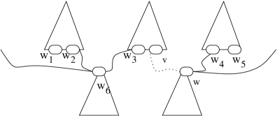
Figure 2: $v$ is the $\mbox{{{S}}}_{b_{i}}$-labeled node whose contents are to be changed by $\mbox{{{S}}}_{c_{i}}[b_{i}/c_{i}]$. The node $w$ is $\mbox{{{S}}}_{c_{i}}$-labeled, and will be “linked” to node $v$ after step $i+1$ of prune procedure is finished — signified by the dotted line. Solid lines represent links that have been established in step $j<i+1$ of the procedure.

This is a snapshot of the moment just before we apply step $i+1$. Step $i$ of prune procedure simply prunes the subtree rooted at the $\mbox{{{S}}}_{b_{i}}$-labeled node $v$, and links (rejustifies) $v$ using the $\mbox{{{S}}}_{c_{i}}$-labeled node $w$, where $b_{i}$ and $c_{i}$ belong to the same equivalence class in $\mbox{{{J}}}_{i}$. It is important to note that some cousin $w_{3}$ of $v$ might also be linked to a root $w_{6}$ of another tree, which in turn might be linked to a leaf node $w_{2}$ of another tree, which in turn might have a cousin $w_{1}$ that satisfies the same property as $w_{3}$ and so on. Furthermore, the node $w$ might have also been linked to some other leaf $w_{4}$ that has a cousin $w_{5}$ that is connected to a root of some other tree, and so on. Note that it is impossible for two leafs of a tree to be linked to the same root node of a tree by construction. Hence, the three trees in the middle (i.e. where $v,w$, and $w_{6}$ are located) are necessarily distinct. The leftmost and rightmost tree might be the same tree depending on the value of the girth $g$ that we defined earlier.

Let us now define

A $$\overset{\mbox{\tiny def}}{=} \{t\in\mbox{{{L}}}:d_{\mathbb{G}(\mbox{{{J}}}_{i})}(t,b_{i})\leq m\}$$

B $$\overset{\mbox{\tiny def}}{=} \{t\in\mbox{{{L}}}:d_{\mathbb{G}(\mbox{{{J}}}_{i})}(t,\mbox{{{S}}}_{c_{i}})\leq m\}.$$

Intuitively, the set A contains tuples up to distance $m$ from the label $\mbox{{{S}}}_{b_{i}}$ of node $v$ in $\mbox{{J}}_{i}$, while the set B contains tuples up to distance $m$ from the label $\mbox{{{S}}}_{c_{i}}$ of $w$ in $\mbox{{J}}_{i}$. Note that this is distance in the structure $\mbox{{J}}_{i}$, not $\mbox{{J}}_{i+1}$. It is immediate that we have property (2) $\mbox{{{A}}}\cup\mbox{{{B}}}=\mbox{{{L}}}$, as the length of the view $V$ is at most $m$ and that $adom(\mbox{{{M}}}_{b_{i}})\subseteq\{b_{i}\}\cup adom(\mbox{{{S}}}_{c_{i}})$. So, it is sufficient to show that properties 3 and 5 are satisfied, as they obviously imply properties 1 and 4. Note that our construction has ensured that:

1. Two nodes in any given tree in $\mathcal{K}_{i}$ that are at least distance two apart cannot share a constant.

2. Two trees $T$ and $T^{\prime}$ in $\mathcal{K}_{i}$ cannot share a constant except on: (i) a unique leaf of $T$ and the root of $T^{\prime}$, as is the case for $v$ and $w$ in Figure 2 or alternatively (ii) a unique leaf of $T$ and a unique leaf of $T^{\prime}$. This case can happen when both leafs are connected to the root of a different tree $T^{\prime\prime}$, as is the situation for $w_{2}$ and $w_{3}$ in Figure 2.

Therefore, for some sufficiently large constant $c^{\prime}\in\mathbb{N}$, two nodes $v^{\prime}$ and $v^{\prime\prime}$ in $\mathcal{K}_{i}$ of distance $c^{\prime}m$ cannot have two elements of $\mbox{{{J}}}_{i}$ that are of distance $\leq m$ in $\mathbb{G}(\mbox{{{J}}}_{i})$. [In fact, a careful analysis will show that $c^{\prime}=1$ is sufficient.] Therefore, the locations of the constants in A (resp. B) cannot be “very far away” from the tuple $v$ (resp. $w$). In fact, if we set $c\geq c^{\prime}$ (recall that $g=cm$) and consider the path $P$ between a tuple $t\in\mbox{{{A}}}$ and the constant $b_{i}$ (which belongs to $v$ and its parent), it cannot connect a root and a leaf of the same tree (i.e. through the body of the tree). So, either it is completely contained in the tree of which $v$ is a leaf, or it has to alternate alternate between leafs and root several times, and then end in some tree. In figure 2, we may pick the following example

$$v\rightarrow^{*}w_{3}\rightarrow w_{6}\rightarrow w_{2}\rightarrow^{*}w_{1}\rightarrow\ldots,$$

where we use the notation $\rightarrow^{*}$ to mean “path in the same tree”. The same analysis can be applied to determine the locations of the tuples of B. Therefore, in order the ensure that properties 3 and 5 are satisfied, we just need to ensure that the height of each tree and the girth of $\mathcal{K}_{i}$ be large enough, which can be done by taking a sufficiently large $c$. When the girth (as ensured in the copy and prune procedures) is sufficiently large, we can be sure that no paths of length $\leq m$ exist between $v$ and $w$ in $\mathcal{K}_{i}$ [In fact, a careful but tedious analysis shows that $c=1$ is sufficient.] ∎

Theorem 4.1 also holds for infinite models, since even if the initial justification hierarchies are infinite, the proof method used is unchanged. We thus also obtain finite controllability (every satisfiable formula is finitely satisfiable) for UCV.

Proposition 4.16

The UCV class of formulas is finitely controllable.

5 Extending the View Definitions

The previous section showed that the first order language using unary conjunctive view definitions is decidable. A natural way to increase the power of the language is to make view bodies more expressive (but retain unary arity for the views). We say earlier that allowing unary views to use disjunction in their definition does not actually increase expressiveness of the UCV language and hence this case is decidable. Unfortunately, as we will show, employing other ways of extending the views results in satisfiability becoming undecidable.

The first extension we consider is allowing inequality in the views, e.g.,

$V(x)\leftarrow R(x,y),S(x,x),x\neq y$

Call the first order language over such views the first order unary conjunctive^≠ view language. In fact, this language allows us to check whether a two counter machine computation is valid and terminates, which thus leads to the following result:

Theorem 5.1

Satisfiability is undecidable for the first order unary conjunctive^≠ view query language.

Proof.

The proof is by a reduction from the halting problem of two counter machines (2CM’s) starting with zero in the counters. Given any description of a 2CM and its computation, we can show how to a) encode this description in database relations and b) define queries to check this description. We construct a query which is satisfiable iff the 2CM halts. The basic idea of the simulation is similar to one in [Levy et al. (1993)], but with the major difference that cycles are allowed in the successor relation, though there must be at least one good chain.

A two-counter machine is a deterministic finite state machine with two non-negative counters. The machine can test whether a particular counter is empty or non-empty. The transition function has the form

$$\delta:\;S\;\times\;\{=,>\}\;\times\;\{=,>\}\;\rightarrow\;S\;\times\;\{pop,push\}\;\times\;\{pop,push\}$$

For example, the statement $\delta(4,=,>)\;=\;(2,push,pop)$ means that if we are in state 4 with counter 1 equal to 0 and counter 2 greater than 0, then go to state 2 and add one to counter 1 and subtract one from counter 2.

The computation of the machine is stored in the relation $config(t,s,c_{1},c_{2})$, where $t$ is the time, $s$ is the state and $c_{1}$ and $c_{2}$ are values of the counters. The states of the machine can be described by integers $0,1\ldots,h$ where 0 is the initial state and $h$ the halting (accepting) state. The first configuration of the machine is $config(0,0,0,0)$ and thereafter, for each move, the time is increased by one and the state and counter values changed in correspondence with the transition function.

We will use some relations to encode the computation of 2CMs starting with zero in the counters. These are:

• $S_{0},\ldots,S_{h}$: each contains a constant which represents that particular state.

• $succ$: the successor relation. We will make sure it contains one chain starting from $zero$ and ending at $last$ (but it may in addition contain unrelated cycles).

• $config$: contains computation of the 2CM.

• $zero$: contains the first constant in the chain in $succ$. This constant is also used as the number zero.

• $last$: contains the last constant in the chain in $succ$.

Note that we sometimes blur the distinction between unary relations and unary views, since a view $V$ can simulate a unary relation $U$ if it is defined by $V(x)\leftarrow U(x)$.

The unary and nullary views (the latter can be eliminated using quantified unary views) are:

• $halt$: true if the machine halts.

• $bad$: true if the database doesn’t correctly describe the computation of the 2CM.

• $dsucc$: contains all constants in $succ$.

• $dT$: contains all time stamps in $config$.

• $dP$: contains all constants in $succ$ with predecessors.

• $dCol_{1},dCol_{2}$: are projections of the first and second columns of $succ$.

When defining the views, we also state some formulas (such as $hasPred$) over the views which will be used to form our first order sentence over the views.

• The “domain” views (those starting with the letter $d$) are easy to define, e.g.

  $dP(x)\leftarrow succ(z,x)$

  $dCol_{1}(x)\leftarrow succ(x,y)$

  $dCol_{2}(x)\leftarrow succ(y,x)$

• $hasPred$ says “each nonzero constant in $succ$ has a predecessor:”

  $hasPred:$ $\forall x(dsucc(x)\Rightarrow(zero(x)\vee\ dP(x)))$

• $sameDom$ says “the constants used in $succ$ and the timestamps in $config$ are the same set”:

  $sameDom:$ $\forall x(dsucc(x)\Rightarrow dT(x))\wedge\forall y(dT(y)\Rightarrow dsucc(y)))$

• $goodzero$ says “the zero occurs in $succ$”:

  $goodzero:$ $\forall x(zero(x)\Rightarrow dsucc(x))$

• $nempty$ : each of the domains and unary base relations is not empty

  $nempty:$ $\exists x(dsucc(x))$

• Check that each constant in $succ$ has at most one successor and at most one predecessor and that it has no cycles of length 1.

  $bad\leftarrow succ(x,y),succ(x,z),y\neq z$

  $bad\leftarrow succ(y,x),succ(z,x),y\neq z$

  $bad\leftarrow succ(x,x)$

  Note that the first two of these rules could be enforced by database style functional dependencies $x\rightarrow y$ and $y\rightarrow x$ on $succ$.

• Check that every constant in the chain in succ which isn’t the last one must have a successor

  $hassuccnext:$ $\forall y(dCol_{2}(y)\Rightarrow(last(y)\vee dCol_{1}(y))$

• Check that the last constant has no successor and zero (the first constant) has no predecessor.

  $bad\leftarrow last(x),succ(x,y)$

  $bad\leftarrow zero(x),succ(y,x)$

• Check that every constant eligible to be in last and zero must be so.

  $eligiblezero:$ $\forall y(dCol_{1}(y)\Rightarrow(dCol_{2}(y)\vee zero(y))$

  $eligiblelast:$ $\forall y(dCol_{2}(y)\Rightarrow(dCol_{1}(y)\vee last(y)))$

• Each $S_{i}$ and $zero$ and $last$ contain $\leq$ 1 element.

  $bad\leftarrow S_{i}(x),S_{i}(y),x\neq y$

  $bad\leftarrow zero(x),zero(y),x\neq y$

  $bad\leftarrow last(x),last(y),x\neq y$

• Check that $S_{i},S_{j},last,zero$ are disjoint ($0\leq i<j\leq h$):

  $bad\leftarrow zero(x),last(x)$

  $bad\leftarrow S_{i}(x),S_{j}(x)$

  $bad\leftarrow zero(x),S_{i}(x)$

  $bad\leftarrow last(x),S_{i}(x)$

• Check that the timestamp is the key for $config$. There are three rules, one for the state and two for the two counters; the one for the state is:

  $bad\leftarrow config(t,s,c_{1},c_{2}),$$config(t,s^{\prime},c^{\prime}_{1},c^{\prime}_{2}),s\neq s^{\prime}$

• Check the configuration of the 2CM at time zero. $config$ must have a tuple at $(0,0,0,0)$ and there must not be any tuples in config with a zero state and non zero times or counters.

  $V_{z_{s}}(s)\!\leftarrow\!zero(t),\!config(t,s,x,y)$

  $V_{z_{c_{1}}}(c)\!\leftarrow\!zero(t),\!config(t,x,c,y)$

  $V_{z_{c_{2}}}(c)\!\leftarrow\!zero(t),\!config(t,x,y,c)$

  $V_{y_{s}}(t)\!\leftarrow\!zero(s),\!config(t,s,x,y)$

  $V_{y_{c_{1}}}(c_{1})\!\leftarrow\!zero(s),\!config(t,s,c_{1},x)$

  $V_{y_{c_{2}}}(c_{2})\!\leftarrow\!zero(s),\!config(t,s,x,c_{2})$

  $goodconfigzero:$ $\forall x(V_{z_{s}}(x)\Rightarrow S_{0}(x)\wedge$

  $(V_{z_{c_{1}}}(x)\vee V_{z_{c_{2}}}(x)\vee V_{y_{s}}(x)\vee V_{y_{c_{1}}}(x)\vee V_{y_{c_{2}}}(x))\Rightarrow zero(x))$

• For each tuple in $config$ at time $t$ which isn’t the halt state, there must also be a tuple at time $t+1$ in $config$.

  $V_{1}(t)\leftarrow config(t,s,c_{1},c_{2}),S_{h}(s)$

  $V_{2}(t)\leftarrow succ(t,t2),config(t2,s^{\prime},c_{1}^{\prime},c_{2}^{\prime})$

  $hasconfignext:$ $\forall t((dt(t)\wedge\neg V_{1}(t))\Rightarrow V_{2}(t))$

• Check that the transitions of the 2CM are followed. For each transition $\delta(j,>,=)=(k,pop,push)$, we include three rules, one for checking the state, one for checking the first counter and one for checking the second counter. For the transition in question we have for checking the state

  $V_{\delta}(t^{\prime})\leftarrow config(t,s,c_{1},c_{2}),succ(t,t^{\prime}),S_{j}(s),succ(x,c_{1}),zero(c_{2})$

  $V_{\delta_{s}}(s)\leftarrow V_{\delta}(t),config(t,s,c_{1},c_{2})$

  $goodstate_{\delta}:$ $\forall s(V_{\delta_{s}}(s)\Leftrightarrow S_{k}(s))$

  and for the first counter, we (i) find all the times where the transition is definitely correct for the first counter

  $$\begin{array}[]{@{}r@{~}l}Q_{1_{\delta}}(t^{\prime})~{}&\leftarrow config(t,s,c_{1},c_{2}),\\ ~{}&\;\;\;succ(t,t^{\prime}),S_{j}(s),succ(x,c_{1}),\\ ~{}&\;\;\;zero(c_{2}),succ(c_{1}^{\prime\prime},c_{1}),config(t^{\prime},s^{\prime},c_{1}^{\prime\prime},c_{2}^{\prime})\mbox{\Large}\end{array}$$

  (ii) find all the times where the transition may or may not be correct for the first counter

  $$Q_{2_{\delta}}(t^{\prime})\leftarrow config(t,s,c_{1},c_{2}),succ(t,t^{\prime}),S_{j}(s),succ(x,c_{1}),zero(c_{2})$$

  and make sure $Q_{1_{\delta}}$ and $Q_{2_{\delta}}$ are the same

  $goodtrans_{\delta_{c_{1}}}:$ $\forall t(Q_{1_{\delta}}(t)\Leftrightarrow Q_{2_{\delta}}(t))$

  Rules for second counter are similar.

  For transitions $\delta_{1},\delta_{2},\ldots,\delta_{k}$, the combination can be expressed thus:

  $goodstate:$ $goodstate_{\delta_{1}}\wedge goodstate_{\delta_{2}}\wedge\ldots\wedge goodstate_{\delta_{k}}$

  $goodtrans_{c_{1}}:$ $goodtrans_{\delta_{1_{c_{1}}}}\wedge goodtrans_{\delta_{2_{c_{1}}}}\wedge\ldots\wedge goodtrans_{\delta_{k_{c_{1}}}}$

  $goodtrans_{c_{2}}:$ $goodtrans_{\delta_{1_{c_{2}}}}\wedge goodtrans_{\delta_{2_{c_{2}}}}\wedge\ldots\wedge goodtrans_{\delta_{k_{c_{2}}}}$

• Check that halting state is in $config$.

  $hlt(t)\leftarrow config(t,s,c_{1},c_{2}),S_{h}(s)$

  $halt:$ $\exists xhlt(x)$

Given these views, we claim that satisfiability is undecidable for the query $\psi=\neg bad\wedge hasPred\wedge sameDom\wedge halt\wedge goodzero\wedge goodconfigzero\wedge\wedge nempty\wedge hassuccnext\wedge eligiblezero\wedge eligiblelast\wedge goodstate\wedge goodtrans_{c_{1}}\wedge goodtrans_{c_{2}}\wedge hasconfignext$ ∎

The second extension we consider is to allow “safe” negation in the conjunctive views, e.g.

$V(x)\leftarrow R(x,y),R(y,z),\neg R(x,z)$

Call the first order language over such views the first order unary conjunctive^¬ view language. It is also undecidable, by a result in [Bailey et al. (1998)].

Theorem 5.2

[Bailey et al. (1998)] Satisfiability is undecidable for the first order unary conjunctive^¬ view query language.   

A third possibility for increasing the expressiveness of views would be to keep the body as a pure conjunctive query, but allow views to have binary arity, e.g.

$V(x,y)\leftarrow R(x,y)$

This doesn’t yield a decidable language either, since this language has the same expressiveness as first order logic over binary relations, which is known to be undecidable [Börger et al. (1997)].

Proposition 5.3

Satisfiability is undecidable for the first order binary conjunctive view language.   

A fourth possibility is to use unary conjunctive views, but allow recursive view definitions. e.g.

$V(x)\leftarrow edge(x,y)$

$V(x)\leftarrow V(x)\wedge edge(y,x)$

Call this the first order unary conjunctive^rec language. This language is undecidable also.

Theorem 5.4

Satisfiability is undecidable for the first order unary conjunctive^rec view language.

Proof.

(sketch): The proof of theorem 5.1 can be adapted by removing inequality and instead using recursion to ensure there exists a connected chain in $succ$. It then becomes more complicated, but the main property needed is that $zero$ is connected to $last$ via the constants in $succ$. This can be expressed by

$conn\_zero(x)\leftarrow zero(x)$

$conn\_zero(x)\leftarrow conn\_zero(y),succ(y,x)$

$\exists x(last(x)\wedge conn\_zero(x))$

∎

6 Applications

6.1 Reasoning Over Ontologies

A currently active area of research is that of reasoning over ontologies (see e.g. [Horrocks (2005)]). The aim here is to use decidable query languages used for accessing and reasoning about information and structure for the Semantic Web. In particular, ontologies provide vocabularies which can define relationships or associations between various concepts (classes) and also properties that link different classes together. Description logics are a key tool for reasoning over schemas and ontologies and to this end, a considerable number of different description logics have been developed. To illustrate some reasoning over a simple ontology, we adopt an example from [Horrocks et al. (2003)], describing people, countries and some relationships. This example can be encoded in a description logic such as $SHIQ$ and also in the UCV query language. We show how to accomplish the latter.

• Define classes such as $Country,Person,Student$ and $Canadian$. These are just unary views defined over unary relations, e.g. $Country(x)\leftarrow country(x)$. Observe that we can blur the distinction between unary views and unary relations and use them interchangeably.

• State that $student$ is a subclass of $Person$.

  $$\forall xStudent(x)\Rightarrow Person(x)$$

• State that $Canada$ and $England$ are both instances of the class $Country$. To accomplish this in the UCV language, we could define $Canada$ and $England$ as unary views and ensure that they are contained in the $Country$ relation and are disjoint with all other classes/instances.

• Declare $Nationality$ as a property relating the classes $Person$ (its domain) and $Country$ (its range). In the UCV language, we could model this as a binary relation $Nationality(x,y)$ and impose constraints on its domain and range. e.g.

  $dom\_Nationality(x)\leftarrow Nationality(x,y)$

  $range\_Nationality(y)\leftarrow Nationality(x,y)$

  $\forall x(dom\_Nationality(x)\Rightarrow Person(x))$

  $\forall x(range\_Nationality(x)\Rightarrow Country(x))$

• State that $Country$ and $Person$ are disjoint classes. $\forall x(Country(x)\Rightarrow\neg Person(x))$.

• Assert that the class $Stateless$ is defined precisely as those members of the class $Person$ that have no values for the property $Nationality$.

  $has\_Nationality(x)\leftarrow Nationality(x,y)$

  $Stateless(x)\Leftrightarrow Person(x)\wedge\neg has\_Nationality(x)$

The above types of statements are reasonably simple to express. In order to achieve more expressiveness, property chaining and property composition have been identified as important reasoning features. To this end, integration of rule-based KR and DL-based KR is an active area of research. The UCV query language has the advantage of being able to express certain types of property chaining, which would not be expressible in the description logic SHIQ, which is not able to accomplish chaining [Horrocks et al. (2003)]. For example

• An uncle is precisely a parent’s brother.

  $uncle_{1}(z)\leftarrow parent(x,y),brother(x,z)$

  $uncle_{2}(z)\leftarrow parent(x,y),brother(z,x)$

  $uncle(z)\Leftrightarrow uncle_{1}(z)\vee uncle_{2}(z)$

We consequently believe the UCV query language has some intriguing potential to be used as a reasoning component for ontologies, possibly to supplement description logics for some specialized applications. We leave this as an open area for future investigation.

6.2 Containment and Equivalence

We now briefly examine the application of our results to query containment. Theorem 4.1 implies we can test whether $Q_{1}(x)\subseteq Q_{2}(x)$ under the constraints $C_{1}\wedge C_{2}\ldots\wedge C_{n}$ where $Q_{1},Q_{2},C_{1},\ldots,C_{n}$ are all first order unary conjunctive view queries in 2-NEXPTIME. This just amounts to testing whether the sentence $\exists x(Q_{1}(x)\wedge\neg Q_{2}(x))\wedge C_{1}\wedge\ldots\wedge C_{n}$ is unsatisfiable. Equivalence of $Q_{1}(x)$ and $Q_{2}(x)$ can be tested with containment tests in both directions.

Of course, we can also show that testing the containment $Q_{1}\subseteq Q_{2}$ is undecidable if $Q_{1}$ and $Q_{2}$ are first order unary conjunctive view^≠ queries, first order unary conjunctive view^¬ queries and first order unary conjunctive^rec view queries.

Containment of queries with negation was first considered in [Sagiv and Yannakakis (1980)]. There it was essentially shown that the problem is decidable for queries which do not apply projection to subexpressions with difference. Such a language is disjoint from ours, since it cannot express a sentence such as $\exists yV_{4}(y)\wedge\neg\exists x(V_{1}(x)\wedge\neg V_{2}(x))$ where $V_{1}$ and $V_{2}$ are views defined over several variables.

6.3 Inclusion Dependencies

Unary inclusion dependencies were identified as useful in [Cosmadakis et al. (1990)]. They take the form $R[x]\subseteq S[y]$. If we allow $R$ and $S$ above to be unary conjunctive view queries, we could obtain unary conjunctive view containment dependencies. Observe that the unary views are actually unary projections of the join of one or more relations.

We can also define a special type of dependency called a proper first order unary conjunctive inclusion dependency, having the form $Q_{1}(x)\subset Q_{2}(x)$, where $Q_{1}$ and $Q_{2}$ are first order unary conjunctive view queries with one free variable. If $\{d_{1},\ldots,d_{k}\}$ is a set of such dependencies, then it is straightforward to test whether they imply another dependency $d_{x}$, by testing the satisfiability of an appropriate first order unary conjunctive view query.

Theorem 6.1

Implication for the class of unary conjunctive view containment dependencies with subset and proper subset operators is i) decidable in 2-NEXPTIME and ii) finitely controllable.   

The results from [Cosmadakis et al. (1990)] show that implication is decidable in polynomial time, but not finitely controllable, for either of the combinations i) functional dependencies plus unary inclusion dependencies, ii) full implication dependencies plus unary inclusion dependencies. In contrast, the stated complexity in the above theorem is much higher, due to the increased expressiveness of the dependencies, yet interestingly the class is finitely controllable.

We might also consider unary conjunctive^≠ containment dependencies. The tests in the proof of theorem 5.1 for the 2CM can be written in the form $Q_{1}(x)\subseteq Q_{2}(x)$, with the exception of the non-emptiness constraints, which must use the proper subset operator. Interestingly also, we can see from the proof of theorem 5.1, that adding the ability to express functional dependencies would also result in undecidability. We can summarise these observations in the following theorem and its corollary.

Theorem 6.2

Implication is undecidable for unary conjunctive^≠ (or conjunctive^¬) view containment dependencies with the subset and the proper subset operators.   

Corollary 6.3

Implication is undecidable for the combination of unary conjunctive view containment dependencies plus functional dependencies.

6.4 Active Rule Termination

The languages in this paper have their origins in [Bailey et al. (1998)], where active database rule languages based on views were studied. The decidability result for first order unary conjunctive views can be used to positively answer an open question raised in [Bailey et al. (1998)], which essentially asked whether termination is decidable for active database rules expressed using unary conjunctive views.

7 Expressive Power of the UCV Language

As we have seen in the previous sections, the logic UCV is quite suitable to reason about hereditary information such as “$x$ is a grandchild of $y$” over family trees. This is due to the fact that UCV can express the existence of a directed walk of length $k$ in the graph, for any fixed positive integer $k$. Therefore, it is natural to also ask what is inexpressible in the logic. In this section, we describe a game-theoretic technique for proving inexpressibility results for UCV. First, we show an easy adaptation of Ehrenfeucht-Fraïssé  games for proving that a boolean query is inexpressible in $\text{UCV}(\sigma,\mathcal{V})$ for a signature $\sigma$ and a finite view set $\mathcal{V}$ over $\sigma$. Second, we extend this result for proving that a boolean query is inexpressible in $\text{UCV}(\sigma)$. An inexpressibility result of the second kind is clearly more interesting, as it is independent of our choice of the view set $\mathcal{V}$ over $\sigma$. Moreover, such a result places an ultimate limit of what can be expressed by UCV queries. Although it can be adapted to any class $\mathcal{C}$ of structures, we shall only state our theorem for proving inexpressibility results in UCV over all finite structures. For this section only, we shall use $STRUCT(\sigma)$ to denote the set of all finite $\sigma$-structures.

Our first goal is quite easy to achieve. Recall that each view set $\mathcal{V}$ over $\sigma$ induces a mapping $\Lambda:STRUCT(\sigma)\rightarrow STRUCT(\mathcal{V})$ as defined in section 2.

Theorem 7.1

Let $\mbox{{{A}}},\mbox{{{B}}}\in STRUCT(\sigma)$. Define the function $\Lambda:STRUCT(\sigma)\rightarrow STRUCT(\mathcal{V})$. Then, the following statements are equivalent:

1. A and B agree on $\text{UCV}(\sigma,\mathcal{V})$.

2. $\Lambda(\mbox{{{A}}})\equiv_{1}^{\text{UFO}(\mathcal{V})}\Lambda(\mbox{{{B}}})$ (i.e. they agree on $\text{UFO}(\mathcal{V})$ formulas of quantifier rank 1.

Proof.

Immediate from lemma 2.1, and lemma 3.1. ∎

So, to prove that a boolean query $\mathcal{Q}$ is not expressible in $\text{UCV}(\sigma,\mathcal{V})$, it suffices to find two $\sigma$-structures such that $\Lambda(\mbox{{{A}}})\equiv_{1}^{\text{UFO}(\mathcal{V})}\Lambda(\mbox{{{B}}})$, but A and B do not agree on $\mathcal{Q}$. In turn, to show that $\Lambda(\mbox{{{A}}})\equiv_{1}^{\text{UFO}(\mathcal{V})}\Lambda(\mbox{{{B}}})$, we can use Ehrenfeucht-Fraïsse games.

We now turn to the second task. Let us begin by stating an obvious corollary of the preceding theorem.

Corollary 7.2

Let $\mbox{{{A}}},\mbox{{{B}}}\in STRUCT(\sigma)$. For any view set $\mathcal{V}$, define the function $\Lambda^{\mathcal{V}}:STRUCT(\sigma)\rightarrow STRUCT(\mathcal{V})$. Then, the following statements are equivalent:

1. A and B agree on $\text{UCV}(\sigma)$.

2. For any view set $\mathcal{V}$ over $\sigma$, we have $\Lambda^{\mathcal{V}}(\mbox{{{A}}})\equiv_{1}^{\text{UFO}(\mathcal{V})}\Lambda^{\mathcal{V}}(\mbox{{{B}}})$

This corollary is not of immediate use. Namely, checking the second statement is a daunting task, as there are infinitely many possible view sets $\mathcal{V}$ over $\sigma$. Instead, we shall propose a sufficient condition for this, which employs the easy direction of the well-known homomorphism preservation theorem (see [Hodges (1997)]).

Definition 7.3.

A formula $\phi$ over a vocabulary $\sigma$ is said to be preserved under homomorphisms, if for any $\mbox{{{A}}},\mbox{{{B}}}\in STRUCT(\sigma)$ the following statement holds: whenever $\mbox{{{a}}}\overset{\mbox{\tiny def}}{=}(a_{1},\ldots,a_{m})\in\phi(\mbox{{{A}}})$ and $h$ is a homomorphism from A to B, it is the case that $h(\mbox{{{a}}})\overset{\mbox{\tiny def}}{=}(h(a_{1}),\ldots,h(a_{m}))\in\phi(\mbox{{{B}}})$.

Lemma 7.4

Conjunctive queries are preserved under homomorphisms.

Theorem 7.5

Let $\mbox{{{A}}},\mbox{{{B}}}\in STRUCT(\sigma)$. To prove that $\Lambda(\mbox{{{A}}})\equiv_{1}^{\text{UFO}(\mathcal{V})}\Lambda(\mbox{{{B}}})$ for all $\sigma$-view sets $\mathcal{V}$, it is sufficient to show that

1. For every $a\in A$, there exists a homomorphism $h$ from A to B and a homomorphism $g$ from B to A such that $g(h(a))=a$.

2. For every $b\in B$, there exists a homomorphism $h$ from A to B and a homomorphism $g$ from B to A such that $h(g(b))=b$.

Proof.

Take an arbitrary $\sigma$-view set $\mathcal{V}$. We use Ehrenfeucht-Fraïsse game argument. Suppose Spoiler places a pebble on an element $a$ of $\Lambda(\mbox{{{A}}})$, whose domain is $A$. Then, the first assumption tells us that there exist homomorphisms $h:A\rightarrow B$ and $g:B\rightarrow A$ such that $g(h(a))=a$. Duplicator may respond by placing the other pebble from the same pair on the element $h(a)$ of $\Lambda(\mbox{{{B}}})$. To show this, we need to prove that $a\mapsto h(a)$ defines an isomorphism between the substructures of $\Lambda(\mbox{{{A}}})$ and $\Lambda(\mbox{{{B}}})$ induced by, respectively, the sets $\{a\}$ and $\{h(a)\}$. Let $V\in\mathcal{V}$. It is enough to show that $a\in V(\mbox{{{A}}})$ iff $h(a)\in V(\mbox{{{B}}})$. If $a\in V(\mbox{{{A}}})$, then we have $h(a)\in V(\mbox{{{B}}})$ by lemma 7.4. Similarly, if $h(a)\in V(\mbox{{{B}}})$, theorem 7.4 implies that $a=g(h(a))\in V(\mbox{{{A}}})$.

For the case where Spoiler plays an element of B, we can use the same argument with the aid of the second assumption above. In either case, we have $\Lambda(\mbox{{{A}}})\equiv_{1}\Lambda(\mbox{{{B}}})$. ∎

This theorem allows us to give easy inexpressibility proofs for a variety of first-order queries. We now give three easy inexpressibility proofs for first-order queries over directed graphs (i.e. structures with one binary relation $E$).

Example 7.1.

We show that the formula $SYM\equiv\forall x,y(E(x,y)\leftrightarrow E(y,x))$ accepting graphs with symmetric $E$ is not expressible in $\text{UCV}(\sigma)$. To do this, consider the graphs A and B defined as follows

Obviously, the graph $E^{\mbox{{{A}}}}$ is symmetric, while $E^{\mbox{{{B}}}}$ is not. Consider the functions $h_{1},h_{2}:A\rightarrow B$ and $g:B\rightarrow A$ defined as

• $h_{1}(a)=h_{1}(c)=a$ and $h_{1}(b)=h_{1}(d)=b$,

• $h_{2}(a)=h_{2}(c)=c$ and $h_{2}(b)=h_{2}(d)=d$, and

• for $i\in B$, $g(i)=i$.

It is easy to verify that $h_{1}$ and $h_{2}$ are homomorphisms from A to B, whereas $g$ a homomorphism from B to A. Now, for $x\in\{a,b\}$, we have $g(h_{1}(x))=x$ and $h_{1}(g(x))=x$. For $x\in\{c,d\}$, we have $g(h_{2}(x))=x$ and $h_{2}(g(x))=x$. So, by theorem 7.5 and corollary 7.2, we conclude that $SYM$ is not expressible in $\text{UCV}(\sigma)$ over all finite directed graphs.

Example 7.2.

We now show that the transitivity query

$$TRANS\equiv\forall x,y,z(E(x,y)\wedge E(y,z)\rightarrow E(x,z))$$

is not expressible in $\text{UCV}(\sigma)$. To do this, consider the graphs A and B defined as

It is obvious that $\mbox{{{A}}}\models TRANS$, and it is not the case that $\mbox{{{B}}}\models TRANS$. Consider the homomorphisms $h_{1},h_{2}$ from A to B, and the homomorphism $g$ from B to A defined as

• for $i\in A$, $h_{1}(i)=i$;

• for $i\in A$, $h_{2}(i)=i+3$; and

• for $i\in B$, $g(i)=i\bmod{3}$.

Then, for $i\in A$, we have $g(h_{1}(i))=i$. Conversely, suppose that $i\in B$. If $i=0,1,2$, then $h_{1}(g(i))=i$. Similarly, if $i=3,4,5$, then $h_{2}(g(i))=i$. So, by theorem 7.5 and corollary 7.2, transitivity is not expressible in $\text{UCV}(\sigma)$ over finite directed graphs.

Example 7.3.

The query $\forall x,yE(x,y)$ is also not expressible in $\text{UCV}(\sigma)$. It is easy to apply theorem 7.5 and corollary 7.2 on the following graphs to verify this fact.

8 Related Work

Satisfiability of first order logic has been thoroughly investigated in the context of the classical decision problem [Börger et al. (1997)]. The main thrust there has been determining for which quantifier prefixes first order languages are decidable. We are not aware of any result of this type which could be used to demonstrate decidability of the first order unary conjunctive view language. Instead, our result is best classified as a new decidable class generalising the traditional decidable unary first-order language (the Löwenheim class [Löwenheim (1915)]). Use of the Löwenheim class itself for reasoning about schemas is described in [Theodoratos (1996)], where applications towards checking intersection and disjointness of object oriented classes are given.

As observed earlier, description logics are important logics for expressing constraints on desired models. In [Calvanese et al. (1998)], the query containment problem is studied in the context of the description logic ${\cal DLR}_{reg}$. There are certain similarities between this and the first order (unary) view languages we have studied in this paper. The key difference appears to be that although ${\cal DLR}_{reg}$ can be used to define view constraints, these constraints cannot express unary conjunctive views (since assertions do not allow arbitrary projection). Furthermore, ${\cal DLR}_{reg}$ can express functional dependencies on a single attribute, a feature which would make the UCV language undecidable (see proof of theorem 5.1). There is a result in [Calvanese et al. (1998)], however, showing undecidability for a fragment of ${\cal DLR}_{reg}$ with inequality, which could be adapted to give an alternative proof of theorem 5.1 (although inequality is used there in a slightly more powerful way).

Another interesting family of decidable logics are guarded logics. The Guarded Fragment [Andreka et al. (1998)] and the Loosely Guarded Fragment [Van Bentham (1997)] are both logics that have the finite model property [Hodkinson (2002)]. The philosophy of UCV is somewhat similar to these guarded logics, since the decidability of UCV also arises from certain restrictions on quantifier use. In terms of expressiveness though, guarded logics seem distinct from UCV formulas, not being able to express cyclic views, such as $\exists x(V(x))$, where $V(x)\leftarrow R(x,y),R(y,z),R(z,z^{\prime}),R(z^{\prime},x)$.

Another area of work that deals with complexity of views is the view consistency problem, with results given in [Abiteboul and Duschka (1998)]. This involves determining whether there exists an underlying database instance that realises a specific (bounded) view instance . The problem we have focused on in this paper is slightly more complicated; testing satisfiability of a first order view query asks the question whether there exists an (unbounded) view instance that makes the query true. This explains how satisfiability can be undecidable for first order unary conjunctive^≠ view queries, but view consistency for non recursive datalog^≠ views is in $NP$. Monadic views have been recently examined in [Nash et al. (2007)], where they were shown to exhibit nice properties in the context of answering and rewriting conjunctive queries using only a set of views. This is an interesting counterpoint to the result of this paper, which demonstrate how monadic views can form the basis of a decidable fragment of first order logic.

9 Summary and Further work

In this paper, we have introduced a new decidable language based on the use of unary conjunctive views embedded within first order logic. This is a powerful generalisation of the well known fragment of first order logic using only unary relations (the Löwenheim class). We also showed that our new class is maximal, in the sense that increasing the expressivity of views is not possible without undecidability resulting. Table 1 provides a summary of our decidability results. Note that the Unary Conjunctive^∪ View language corresponds to the extension of UCV by allowing disjunction in the view definition.

We feel that the decidable case we have identified, is sufficiently natural and interesting to be of practical, as well as theoretical interest.

Table 1:
Summary of Decidability Results for First Order View Languages
Unary Conjunctive View Decidable Unary Conjunctive^∪ View Decidable Unary Conjunctive^≠ View Undecidable Unary Conjunctive^rec View Undecidable Unary Conjunctive^¬ View Undecidable [Bailey et al. (1998)] Binary Conjunctive View Undecidable

An interesting open problem for future work is to investigate the decidability of an extension to the first order unary conjunctive view language, when equality is allowed to be used outside of the unary views (i.e. included in the first order part). An example formula in this new language is

$$\forall X,Y(V_{1}(X)\wedge V_{2}(Y)\Rightarrow X\neq Y)$$

We conjecture this extended language is decidable, but do not currently have a proof.

For other future work, we believe it would be worthwhile to investigate relationships with description logics and also examine alternative ways of introducing negation into the UCV language. One possibility might be to allow views of arity zero to specify description logic like constraints, such as $R_{1}(x,y)\subseteq R_{2}(x,y)$.

Finally, there is still an exponential gap between the upper bound complexity of 2-NEXPTIME and lower bound complexity of NEXPTIME-hardness that we derived. The primary reason for this exponential blow-up is the enumeration of all subviews of the views that are present in the formula, which we need for the proof.

We thank Sanming Zhou for pointing out useful references on extremal graph theory. We are grateful to Leonid Libkin for his comments on a draft of this paper.

References

- Abiteboul and Duschka (1998) Abiteboul, S. and Duschka, O. 1998. Complexity of answering queries using materialized views. In Proceedings of the 17th ACM SIGMOD-SIGACT-SIGART Symposium on Principles of Database Systems. Seattle, Washington, 254–263.
- Andreka et al. (1998) Andreka, H., van Bentham, J., and Nemeti, I. 1998. Modal logics and bounded fragments of predicate logics. J. Philosophical Logic 27, 217–274.
- Bailey and Dong (1999) Bailey, J. and Dong, G. 1999. Decidability of first-order logic queries over views. In Proceedings of the International Conference on Database Theory (ICDT). 83–99.
- Bailey et al. (1998) Bailey, J., Dong, G., and Ramamohanarao, K. 1998. Decidability and undecidability results for the termination problem of active database rules. In Proceedings of the 17th ACM SIGMOD-SIGACT-SIGART Symposium on Principles of Database Systems. Seattle, Washington, 264–273.
- Boerger et al. (1996) Boerger, E., Graedel, E., and Gurevich, Y. 1996. The Classical Decision Problem. Springer-Verlag.
- Bollobas (2004) Bollobas, B. 2004. Extremal Graph Theory. Dover Publications.
- Boolos et al. (2002) Boolos, G. S., Burgess, J. P., and Jeffrey, R. C. 2002. Computability and Logic. Cambridge University Press.
- Börger et al. (1997) Börger, E., Grädel, E., and Gurevich, Y. 1997. The Classical Decision Problem. Springer-Verlag.
- Calvanese et al. (1998) Calvanese, D., De Giacomo, G., and Lenzerini, M. 1998. On the decidability of query containment under constraints. In Proceedings of the 17th ACM SIGMOD-SIGACT-SIGART Symposium on Principles of Database Systems. Seattle, Washington, 149–158.
- Cosmadakis et al. (1990) Cosmadakis, S., Kanellakis, P., and Vardi, M. 1990. Polynomial time implication problems for unary inclusion dependencies. Journal of the ACM 37, 1, 15–46.
- Diestel (2005) Diestel, R. 2005. Graph Theory. Springer-Verlag.
- Enderton (2001) Enderton, H. B. 2001. A Mathematical Introduction To Logic. A Harcourt Science and Technology Company.
- Gaifman (1982) Gaifman, H. 1982. On local and nonlocal properties. In Logic Colloquium ’81, J. Stern, Ed. North Holland, 105–135.
- Garcia-Molina et al. (1995) Garcia-Molina, H., Quass, D., Papakonstantinou, Y., Rajaraman, A., and Sagiv, Y. 1995. The tsimmis approach to mediation: Data models and language. In The Second International Workshop on Next Generation Information Technologies and Systems. Naharia, Israel.
- Halevy (2001) Halevy, A. Y. 2001. Answering queries using views: A survey. VLDB Journal: Very Large Data Bases 10, 4, 270–294.
- Hodges (1997) Hodges, W. 1997. A Shorter Model Theory. Cambridge University Press.
- Hodkinson (2002) Hodkinson, I. M. 2002. Loosely guarded fragment of first-order logic has the finite model property. Studia Logica 70, 2, 205–240.
- Horrocks (2005) Horrocks, I. 2005. Applications of description logics: State of the art and research challenges. In Proc. of 13th International Conference on Conceptual Structures (ICCS). 78–90.
- Horrocks et al. (2003) Horrocks, I., Patel-Schneider, P. F., and van Harmelen, F. 2003. From shiq and rdf to owl: the making of a web ontology language. Journal of Web Semantics 1, 1, 7–26.
- Levy et al. (1993) Levy, A., Mumick, I. S., Sagiv, Y., and Shmueli, O. 1993. Equivalence, query reachability, and satisfiability in datalog extensions. In Proceedings of the twelfth ACM SIGACT-SIGMOD-SIGART Symposium on Principles of Database Systems. Washington D.C., 109–122.
- Levy et al. (1996) Levy, A., Rajaraman, A., and Ordille, J. 1996. Querying heterogeneous information sources using source descriptions. In Proceedings of 22th International Conference on Very Large Data Bases. Mumbai, India, 251–262.
- Libkin (2004) Libkin, L. 2004. Elements of Finite Model Theory. Springer-Verlag.
- Löwenheim (1915) Löwenheim, L. 1915. Über möglichkeiten im relativkalkul. Math. Annalen 76, 447–470.
- Nash et al. (2007) Nash, A., Segoufin, L., and Vianu, V. 2007. Determinacy and rewriting of conjunctive queries using views: A progress report. In Proceedings of the International Conference on Database Theory. 59–73.
- Sagiv and Yannakakis (1980) Sagiv, Y. and Yannakakis, M. 1980. Equivalences among relational expressions with the union and difference operators. Journal of the ACM 27, 4, 633–655.
- Theodoratos (1996) Theodoratos, D. 1996. Deductive object oriented schemas. In Proceedings of ER’96, 15th International Conference on Conceptual Modeling. 58–72.
- Ullman (1997) Ullman, J. D. 1997. Information integration using logical views. In Proceedings of the Sixth International Conference on Database Theory, LNCS 1186. Delphi, Greece, 19–40.
- Van Bentham (1997) Van Bentham, J. 1997. Dynamic bits and pieces. Tech. Rep. ILLC Research Report LP-97-01, University of Amsterdam.
- Widom (1995) Widom, J. 1995. Research problems in data warehousing. In Proceedings of the 4th International Conference on Information and Knowledge Management. Baltimore, Maryland, 25–30.