Magnetic barriers in graphene nanoribbons: Theoretical study of transport properties

Abstract

A theoretical study of the transport properties of zigzag and armchair graphene nanoribbons with a magnetic barrier on top is presented. The magnetic barrier modifies the energy spectrum of the nanoribbons locally, which results in an energy shift of the conductance steps towards higher energies. The magnetic barrier also induces $\mathrm{{Fabry-P\acute{e}rot}}$ type oscillations, provided the edges of the barrier are sufficiently sharp. The lowest propagating state present in zigzag and metallic armchair nanoribbons prevent confinement of the charge carriers by the magnetic barrier. Disordered edges in nanoribbons tend to localize the lowest propagating state, which get delocalized in the magnetic barrier region. Thus, in sharp contrast to the case of two-dimensional graphene, the charge carriers in graphene nanoribbons cannot be confined by magnetic barriers. We also present a novel method based on the Green’s function technique for the calculation of the magnetosubband structure, Bloch states and magnetoconductance of the graphene nanoribbons in a perpendicular magnetic field. Utilization of this method greatly facilitates the conductance calculations, because, in contrast to excising methods, the present method does not require self-consistent calculations for the surface Green’s function.

I Introduction

The single planar sheet with carbon atoms densely packed in a honeycomb structure forms the so-called graphene, which demonstrates a variety of unique electronic transport properties and has the potential applications in the future nanoelectronics Neto . Theoretical studies have indicated that the special lattice structure of the graphene results in nearly linear dispersion relations around the K points (Dirac points) of the Brillouin zone Wakabayashi1999 . This unique band structure is responsible for the distinct electronic properties of the graphene. Near the Dirac point, electrons manifest themselves the massless chiral fermions and can be described by the Dirac equation Katsnelson ; Pereira ; Tworzydlo . The electronic transport behaviors of the two-dimensional graphene subjected to an electrostatic potential Katsnelson or a magnetic barrier (MB) Martino were studied on the basis of the Dirac equation, which indicate that the Dirac fermions can be transmitted perfectly through a classically forbidden region while confined effectively by the magnetic barrier. Moreover, the anomalous integer and fractional quantum Hall effects in two-dimensional graphene have been studied experimentally and theoretically by various groups Zhang ; Novoselov ; Peres2006 ; Gusynin .

The rolled-up graphene is known as the single-wall carbon nanotube whose electronic properties have been studied extensively in the past decades. The quantized conductance and $\mathrm{{Fabry-P\acute{e}rot}}$ interference pattern were observed experimentally and interpreted by various theoretical approaches Liang . The other interesting effects including Coulomb blockade Herrero and Kondo effects Nygard , and the electronic transport in ballistic Javey and disordered nanotubes Hjort were studied. Another related carbon-based structure is the graphene nanoribbon (GNR), referred to the quasi-one dimensional graphene with a finite width $W$. Recent development of the experimental technique enable one to fabricate very narrow GNRs with ultrasmooth edges of the width $W\leq 10$ nmLi . The electrons propagate in such narrow systems very differently compared with the two-dimensional graphene where the edges are totally irrelevant. In graphene ribbons, the transport properties are strongly influenced by their edges along the transport direction which are distinguished into two types: zigzag and armchair. For armchair case, it is particularly interesting that the graphene ribbons may be metallic or semiconducting depending on their widths. There is a lot of theoretical effort devoted to the studies of the quantum transport in graphene ribbons. The conductance quantization in mesoscopic graphene Peres2006 and coherent transport in graphene nanoconstrictions with or without defects Munoz-Rojas were reported recently.

The purpose of the present paper is twofold. First, we explore a possibility to control electron conductance of graphene nanoribbons with the help of magnetic barriers. MBs in the conventional quantum wires (QWRs) have been the subject of theoretical and experimental studies, which are driven by the MB’s potential ability of parametric spin filtering. The pioneering theoretical research by Peeters et al. Peeters indicated that the magnetic barrier possesses the wave-vector filtering properties in QWRs and further work in graphene was also suggested Pereira . Furthermore, recent theoretical studies have revealed further rich phenomenology of magnetic barriers in quantum wires, such as Fano-type resonances Xu and spin filtering Majumdar1996 ; Zhai2006 . In two-dimensional graphene, theoretical work has shown the strong effects of the magnetic barrier on the direction-dependent transmission Martino . Our studies will focus on the magnetic barrier effects on the quasi-one-dimensional GNRs.

Second, we present a detailed description of a novel method based on the Green’s function technique for the calculation of the magnetosubband structure, Bloch states and magnetoconductance of the graphene nanoribbons in a perpendicular magnetic field. Note that magnetoconductance calculations for the graphene nanoribbons based on the Green’s function technique has been reported previously Munoz-Rojas ; Datta_Klimeck . However, a distinct feature of the present method is a novel approach to calculation of the surface Green’s function $\Gamma$ for semi-infinite nanoribbons. In contrast to the Green’s functions for finite structures that can be easily calculated by adding slice by slice in a recursive way with the help of the Dyson’s equation, the calculation of the surface Green’s function of a semi-infinite structure represents a non-trivial problem. Such calculations are typically done self-consistently which makes conductance calculations very time-consuming. In the present paper we present a different method of computing $\Gamma$ which does not require self-consistent calculations. Instead, the surface Green’s function is expressed via the Bloch states of the graphene nanoribbons which in turn are simply obtained as solutions of the eigenequation of the dimension $2N\times 2N$ (with $N$ being the width of the nanoribbon). Utilization of this method greatly facilitates the conductance calculations, making the present method far more efficient in comparison to the existing ones. Programming codes for calculation of the magnetosubband structure, the surface Greens function and the magnetoconductance based on the developed method are freely available in the AIP EPAPS electronic depository.EPAPS

This paper is organized as follows: In Sec. II we sketch the geometry of the devices and briefly introduce the model for the conductance for our calculations. In Sec. III, we describe the tight-binding model for the graphene, theory of the Green’s function method, as well as the formalism for the computation of surface Green’s functions. This is followed by the presentation and discussion of the numerical results in Sec. IV. Summary and conclusion constitute the Sec. V.

II Formulation of the problem

The geometries under consideration for graphene nanoribbons with zigzag and armchair edges are illustrated in Fig. 1(b) and (c), respectively, where the left and right leads are made of semi-infinite graphene. The nanoribbons are subjected to a magnetic barrier whose shapes may be rectangular or smooth as shown in Fig. 1(a) with zero magnetic field in leads. (Note however that the theory presented in the next section is not restricted to the case of zero field in the leads). The magnetic barrier represents a strongly localized magnetic field that is oriented perpendicular to the surface of the ribbon. Magnetic barriers with amplitudes up to $1\,\mathrm{T}$ have been realized experimentally by ferromagnetic films on top of a graphene sheet Kubrak2000 ; Cerchez2007 : magnetizing the ferromagnetic film in the transport direction results in a magnetic fringe field with a perpendicular component localized at the edge of the film that extends along the transverse direction. Alternatively, magnetic barrier formation has been demonstrated by placing two-dimensional electron gases with a step in an external magnetic field,Leadbeater1995 an approach which conceptually allows much larger barrier amplitudes. Both concepts should be in principle adaptable to graphene nanoribbons.

Figure 1: Schematic geometry of the structure under consideration for the case of (b) zigzag and (c) armchair graphene. The current through the central part of the device is injected and collected in semi-infinite ideal leads representing graphene nanoribbons of width $N$. Unit cells of the graphene nanoribbons are marked by blue dashed rectangles (see Fig. 2). (a) A ferromagnetic film deposited on the top of the graphene nanoribbons gives rise to an inhomogeneous magnetic field.

We model the leads and the device in the middle by the standard tight-binding Hamiltonian on the honeycomb lattice, see below, Eq. (3). The conductance $\mathbf{G}$ can be calculated using the Landauer-Büttiker formalism which gives the conductance of the system in terms of the electron transmission coefficient $\mathcal{T}$, expressed as

$$\mathbf{G}=-\frac{2e^{2}}{h}\int dE\,\mathcal{T}(E)\frac{\partial f_{FD}\left(E-E_{F}\right)}{\partial E},$$ (1)

where $\mathcal{T}(E)$ is the total transmission coefficient, $f_{FD}(E-E_{F})$ is the Fermi-Dirac distribution function and $E_{F}$ is the Fermi energy.

We calculate the transmission amplitudes of electrons injected to the systems using the recursive Green’s function method which is described in the next section.

III Theory

III.1 Basics

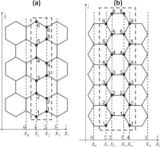
Figure 2: Geometry of (a) zigzag and (b) armchair graphene ribbons. The ribbons are periodic in the $x$-direction (slices in the $x$-directions are labeled by index $i$). The figure shows nanoribbons with $N=6$ sites in the transverse direction. Unit cells of the graphene nanoribbons are marked by dashed rectangles.

We define the Bloch states in the infinite periodic graphene ribbons,

$$|\psi\rangle=\sum_{i,j}\psi_{i,j}a_{i,j}^{+}|0\rangle,\;\psi_{i,j}=e^{ikx_{i}}\varphi_{i,j},$$ (2)

where $a_{i,j}^{+}\,(a_{i,j})$ is a standard creation (annihilation) operator on the site $(i,j)$; $\psi_{i,j}$ is the amplitude of the wave function on the site $(i,j);$ $x_{i}$ is the coordinate of the $i$-th slice, $k$ is the Bloch wave vector in the direction of the translational invariance $x$, and the summation runs over all sites of the graphene lattice (see Fig. 2). Note that this form of the wave function does not distinguish between sublattices A and B of the graphene lattice. An explicit distinction between these sublattices is not necessary when using the Green’s function technique, where, instead, it is more convenient to define the wave function on slices of the lattice (see Sec. III.2).

The standard tight-binding Hamiltonian has the form

$$H=\sum_{r}V_{r}a_{r}^{+}a_{r}-\sum_{r,\Delta}t_{r,r+\Delta}a_{r}^{+}a_{r+\Delta},$$ (3)

where $V_{r}$ describes the electrostatic potential on the site $r=i,j$ and summation in the second term is performed over all available nearest neighbors with $t_{r,r+\Delta}$ being the nearest-neighbor hopping integral. In the absence of a magnetic field the nearest-neighbor hopping integral is $t_{r,r+\Delta}=t_{0}\approx 2.7$ eV. In the presence of an external perpendicular magnetic field $B$ the hopping integral acquires the Peierls phase factor, $t_{r,r+\Delta}=t_{0}\exp(i\theta_{r,r+\Delta}),$where $\theta_{r,r+\Delta}=2\pi\phi_{r,r+\Delta}/\phi_{0}$ , with $\phi_{r,r+\Delta}$ being the line integral of the vector potential $\mathbf{A}$ from site $r$ to a neighboring site $r+\Delta,$

$$\phi_{r,r+\Delta}=\int_{r}^{r+\Delta}\mathbf{A}\cdot d\mathbf{l}$$ (4)

and $\phi_{0}=h/e$ is the flux quantum (in our calculations we use the Landau gauge, $\mathbf{A}=(-By,0)).$ (In calculation of hopping integral (4) we use the carbon-carbon bond length $a=0.142$ nm, see Appendix). Note that the Hamiltonian operator $H$ is convenient to write down in the form,

$$H=\sum_{i}\left[h_{i}\right]+U,$$ (5)

where $h_{i}$ describes the Hamiltonian of the $i$-th slice, and $U$ describes hopping between all neighboring slices (explicit forms of $h_{i}$ and $U$ can be easily obtained from Eq. (3)).

The Green’s function of the operator $H$ is defined in a standard wayDatta_book ; Ferry ,

$$\left(E-H+i\varepsilon\mathcal{\,}\right)G=I$$ (6)

where $I\mathcal{\,}$ is the unitary operator.

III.2 Bloch states and velocities in the graphene nanoribbons.

We continue by describing a method for calculation of the Bloch states and their group velocities in the zigzag and armchair graphene nanoribbons in the presence of a perpendicular magnetic field. The method is based on the technique developed for calculation of the band structure of a mesoscopic antidot lattice in confined geometries Z and has been used for calculation of the Bloch states in photonic structures Rahachou and in the interacting quantum wires in the integer quantum Hall regime wires .

Consider an infinite ideal graphene ribbon with $N$ sites in the transverse $j$-direction, Fig. 2. A unit cell of the structure consists of $M$ slices, where $M=2$ for the zigzag graphene and $M=4$ for the armchair graphene.

The Hamiltonian of an ideal infinitely long graphene ribbon can be written in the form

$$H=H_{\mathrm{cell}}+H_{\mathrm{out}}+U,\mathcal{\,}$$ (7)

where the operators $H_{\mathrm{cell}}$ and $H_{\mathrm{out}}$ describe respectively the unit under consideration ($1\leq i\leq M$), and the outside region including all other slices $-\infty<i\leq 0$ and $M+1\leq i<\infty$, and $U\mathcal{\,}$ is the hopping operator between the cell and slices $i=0$ and $i=M+1$ (an explicit form for these operators can be easily obtained from Eq. (3)). We write the total wave function, Eq. (2), in the form

$$|\psi\rangle=|\psi_{\mathrm{cell}}\rangle+|\psi_{\mathrm{out}}\rangle,$$ (8)

where $|\psi_{\mathrm{cell}}\rangle$ and $|\psi_{\mathrm{out}}\rangle$ are respectively wave functions in the cell and in the outside region. Substituting Eqs. (7),(8) into the Schrödinger equation $H|\psi\rangle=E|\psi\rangle$ and using the definition of the Green’s function, Eq. (6), we obtain $|\psi_{\mathrm{cell}}\rangle=G_{\mathrm{cell}}U|\psi_{\mathrm{out}}\rangle,$ where $G_{\mathrm{cell}}$ is the Green’s function of the operator $H_{\mathrm{cell}}$. Taking the matrix elements of the wave functions in the real space representations, $\psi_{i,j}=\langle 0a_{i,j}|\psi\rangle$ for the first ($i=1$) and the last ($i=M$) slices of the unit cell, this equation can be written in the matrix form,

$$\psi_{1} =G_{\mathrm{cell}}^{1,1}U_{1,0}\psi_{0}+G_{\mathrm{cell}}^{1,M}U_{1,0}^{+}\psi_{M+1}$$ (9)

$$\psi_{M} =G_{\mathrm{cell}}^{M,1}U_{1,0}\psi_{0}+G_{\mathrm{cell}}^{M,M}U_{1,0}^{+}\psi_{M+1},$$

where $\psi_{i}$ is the vector column describing the wave function for the slice $i$,

$$\psi_{i}=\left(\psi_{i,1};\ldots;\psi_{i,N}\right)^{T}$$ (10)

and $U_{1,0}$ and $G_{\mathrm{cell}}^{i,i^{\prime}}$ denote the matrixes with the matrix elements

$$\left(U_{1,0}\right)_{jj^{\prime}} = \langle 0a_{1,j}|U|a_{0,j^{\prime}}^{+}0\rangle$$ (11)

$$\left(G_{\mathrm{cell}}^{i,i^{\prime}}\right)_{jj^{\prime}} = \langle 0a_{i,j}|G_{\mathrm{cell}}|a_{i^{\prime},j^{\prime}}^{+}0\rangle.$$

Explicit expressions for the matrix elements of the matrix $U$ are given in the Appendix. In the derivation of Eq. (9) we used $U_{M,M+1}=U_{0,1}$ (because of the periodicity of the ribbons) and $U_{0,1}=U_{1,0}^{+}$ (‘$+$’ stands for Hermitian conjugate).

It is convenient to rewrite Eq. (9) in a compact form

$$T_{1}\left(\begin{array}[]{c}\psi_{M+1}\\ \psi_{M}\end{array}\right)=T_{2}\left(\begin{array}[]{c}\psi_{1}\\ \psi_{0}\end{array}\right),\;\mathrm{where}$$ (16)

$$T_{1}=\begin{pmatrix}-G_{\mathrm{cell}}^{1,M}U_{1,0}^{+}&\;0\\ -G_{\mathrm{cell}}^{M,M}U_{1,0}^{+}&\;I\end{pmatrix},\;T_{2}=\begin{pmatrix}-I&\;G_{\mathrm{cell}}^{1,1}U_{1,0}\\ 0&\;G_{\mathrm{cell}}^{M,1}U_{1,0}\end{pmatrix}$$

with $I$ being the unitary matrix. The wave function of the periodic structure has the Bloch form,

$$\psi_{m+M}=e^{ikM}I\psi_{m}.$$ (17)

Combining Eqs. (16) and (17), we arrive at the eigenequation,

$$T_{1}^{-1}T_{2}\left(\begin{array}[]{c}\psi_{1}\\ \psi_{0}\end{array}\right)=e^{ikM}\left(\begin{array}[]{c}\psi_{1}\\ \psi_{0}\end{array}\right)$$ (18)

determining the set of Bloch eigenvectors $k_{\alpha}$ and eigenfunctions $\psi^{\alpha},$ $1\leq\alpha\leq N.$ It should be stressed that this eigenequation provides a set of the Bloch states $\left\{k_{\alpha}\right\}$ for a fixed energy $E$, which includes both propagating and evanescent states. The latter can be easily identified by a non-zero imaginary part.

In order to separate right- and left-propagating states, $k_{\alpha}^{+}$ and $k_{a}^{-},$ we compute the group velocities of the Bloch states $v_{\alpha}=\frac{\partial E}{\partial k_{\alpha}}$, whose signs determine the direction of propagation (‘+’ stands for the right-propagating and ‘-’ for the left propagating states). The group velocities can be computed directly by numerical differentiation of the dispersion relation. This is however not an efficient approach because for each energy the eigensolver gives eigenstates $\alpha$ in different order. We instead derive below a simple formula which gives the group velocities of the Bloch states based on the eigenfunctions of Eq. (18).

Consider a unit cell of an infinite graphene nanoribbon consisting of $M$ slices. The wavefunction of the $\alpha$-th Bloch state (2) can be conveniently rewritten in the form $|\psi\rangle=\sum_{i=1}^{M}|\psi_{i}\rangle,$ where $|\psi_{i}\rangle$ is the wave function for the $i$-th slice,

$$|\psi_{i}\rangle=e^{ikx_{i}}|\varphi_{i}\rangle$$ (19)

[To simplify our notations we have dropped the Bloch index $\alpha$ ]. Starting from the Schrödinger equation and calculating the matrix element of the Hamiltonian of the unit cell, we obtain for each slice $i,$ $\langle\psi_{i}|H|\psi\rangle=E\langle\psi_{i}|\psi\rangle=E|\varphi_{i}|^{2}.$ Performing summation over all slices of the unit cell and using a definition of the group velocity, we obtain

$$v=\frac{\partial E}{\partial k}=\frac{1}{M}\sum_{i=1}^{M}\frac{\partial}{\partial k}\left[\frac{\langle\psi_{i}|H|\psi\rangle}{|\varphi_{i}|^{2}}\right]$$ (20)

where the summation is performed over all slices $i$ of the unit cell, and

$$\varphi_{i}=(\varphi_{i,1};...;\varphi_{i,N})^{T}$$ (21)

is a vector composed of the matrix elements $\varphi_{i,j}=$ $\langle 0a_{i,j}|\varphi\rangle.$(Note that according to Eq. (10) and (19), vectors $\varphi_{i}$ can be obtained from $\psi_{i}$ via the relation $\psi_{i}=e^{ikx_{i}}\varphi_{i}$). Representing the Hamiltonian of the unit cell in the form (5), the matrix elements $\langle\psi_{i}|H|\psi\rangle$ can be easily evaluated, which gives

$$v = \frac{-i}{M}\sum_{i=1}^{M}\frac{\varphi_{i}^{\ast T}}{|\varphi_{i}|^{2}}\Big{[}(x_{i}-x_{i-1})U_{i,i-1}\varphi_{i-1}e^{-ik(x_{i}-x_{i-1})}$$ (22)

$$-(x_{i+1}-x_{i})U_{i,i+1}\varphi_{i+1}e^{-ik(x_{i+1}-x_{i})}\Big{]},$$

where the matrixes $U_{i,i^{\prime}}$ are defined by Eq. (11) [explicit expressions for these matrix elements are given in the Appendix].

III.3 Surface Greens function $\Gamma.$

Here, we describe an efficient method for calculation of the surface Green’s function $\Gamma$ in the magnetic field.EPAPS Note that most of the methods for calculation of the Green’s function reported to date require searching for a self-consistent solution for $\Gamma$ which makes these calculation very time consumingMunoz-Rojas ; Datta_Klimeck . In contrast, our method does not require self-consistent calculations, and the surface Greens function is simply given by multiplication of matrixes composed of the Bloch states of the graphene lattice (see below, Eqs. (25),(26)). The calculations described in this section are based on the method developed in Ref. Rahachou for periodic photonic crystals which is adapted here for the case of the graphene nanoribbons.

Consider a semi-infinite periodic ideal graphene ribbon extended to the right in the region $-m\leq i<\infty$. Suppose that an excitation $|s\rangle$ is applied to its surface slice $i=-m$. Introducing the Green’s function of the semi-infinite ribbon, $G_{\mathrm{rib}},$ one can write down the response to the excitation $|s\rangle$ in a standard formDatta_book

$$|\psi\rangle=G_{\mathrm{rib}}|s\rangle,$$ (23)

where $|\psi\rangle$ is the wave function that has to satisfy the Bloch condition (2). Consider a unit cell of a graphene lattice, $1\leq i\leq M,$ ($M=2$ and $4$ for the zigzag and armchair lattices, see Fig. 2). Applying Dyson’s equation between the slices $0$ and $1$ we obtain

$$G_{\mathrm{rib}}^{1,-m}=\Gamma_{r}U_{1,0}G_{\mathrm{rib}}^{0,-m},$$ (24)

where $\Gamma_{r}\equiv G_{\mathrm{rib}}^{1,1}$ is the right surface Green’s function (i.e. the surface function of the semiinfinite ribbon open to the right), and the definition of the matrixes $U$ and $G$ in the real space representation are given by Eq. (11)). Evaluating the matrix elements $\langle 0a_{1,j}|\psi\rangle$ of Eq. (23) and making use of Eq. (24), we obtain for an each Bloch state $\alpha$, $\psi_{1}^{\alpha}=$ $\Gamma_{r}U_{1,0}\psi_{0}^{\alpha}.$ The latter equations can be used for determination of $\Gamma_{r}$,

$$\Gamma_{r}U_{1,0}=\Psi_{1}\Psi_{0}^{-1},$$ (25)

where $\Psi_{1}$ and $\Psi_{0}$ are the square matrixes composed of the matrix-columns $\psi_{1}^{\alpha}$ and $\psi_{0}^{\alpha},$ ($1\leq\alpha\leq N),$ Eq. (18), i.e. $\Psi_{1}=(\psi_{1}^{1},...,\psi_{1}^{N});$ $\Psi_{0}=(\psi_{0}^{1},...,\psi_{0}^{N}).$ The expression for the left surface Greens function $\Gamma_{l}$ (i.e. the surface function of the semiinfinite ribbon open to the right) is derived in a similar fashion,

$$\Gamma_{l}U_{1,0}^{+}=\Psi_{M}\Psi_{M+1}^{-1},$$ (26)

where the matrixes $\Psi_{M}$ and $\Psi_{M+1}$ are defined in a similar way as $\Psi_{1}$ and $\Psi_{0}$ above. Note that matrixes $\Psi_{M}$ and $\Psi_{M+1}$ can be easily obtained from $\Psi_{1}$ and $\Psi_{0}$ using the relation (16). Note also that when the magnetic field is restricted to zero, the right and left surface Greens functions are identical, $\Gamma_{l}=\Gamma_{r}.$

III.4 Magnetoconductance of the graphene nanoribbons

In order to calculate the transmission coefficient $\mathcal{T}(E)$ we divide the structure into three regions, two ideal semi-infinite leads of the width $N$ extending in the regions $i\leq 0$ and $i\geq L$ respectively, and the central device region (where scattering occurs), see Fig. 1. We assume that the left and right leads are identical. The incoming, transmitted and reflected states in the leads, $|\psi_{\alpha}^{\mathrm{i}}\rangle,$ $|\psi_{\alpha}^{\mathrm{t}}\rangle$ and $|\psi_{\alpha}^{\mathrm{r}}\rangle$, have the Bloch form (2),

$$|\psi_{\alpha}^{\mathrm{i}}\rangle =\sum_{i\leq 0}e^{ik_{\alpha}^{+}x_{i}}\sum_{j=1}^{N}\phi_{i,j}^{\alpha}\,a_{i,j}^{+}|0\rangle$$ (27)

$$|\psi_{\alpha}^{\mathrm{t}}\rangle =\sum_{i\geq L}\sum_{\beta}t_{\beta\alpha}e^{ik_{\beta}^{+}(x_{i}-x_{L})}\sum_{j=1}^{N}\phi_{i,j}^{\beta}\,a_{i,j}^{+}|0\rangle$$ (28)

$$|\psi_{\alpha}^{\mathrm{r}}\rangle =\sum_{i\leq 0}\sum_{\beta}r_{\beta\alpha}e^{ik_{\beta}^{-}x_{i}}\sum_{j=1}^{N}\phi_{i,j}^{\beta}\,a_{i,j}^{+}|0\rangle,$$ (29)

where $t_{\beta\alpha}\,(r_{\beta\alpha})$ stands for the transmission (reflection) amplitude from the incoming Bloch state $\alpha$ to the transmitted (reflected) Bloch state $\beta,$ and we choose $x_{0}=0.$ The transmission and reflection coefficients are expressed through the corresponding amplitudes and the Bloch velocitiesDatta_book

$$\mathcal{T}=\sum_{\alpha,\beta}\frac{v_{\beta}}{v_{\alpha}}|t_{\beta\alpha}|^{2};\;\mathcal{R}=\sum_{\alpha,\beta}\frac{v_{\beta}}{v_{\alpha}}|r_{\beta\alpha}|^{2},$$

where the summation runs over propagating states only. The transmission and reflection amplitudes can be calculated from the equationsRahachou ,

$$\Phi_{1}T =-G^{L,0}(U_{0,1}\Phi_{1}K_{1}-{\Gamma_{l}}^{-1}\Phi_{0})$$ (30)

$$\Phi_{0}R =-G^{0,0}(U_{0,1}\Phi_{1}K_{1}-{\Gamma_{l}}^{-1}\Phi_{0})-\Phi_{0}$$ (31)

where the matrixes $T$ and $R$ of the dimension $N\times N_{prop}$ are composed of the transmission and reflection amplitudes $(T)_{\beta\alpha}=t_{\beta\alpha},$ $(R)_{\beta\alpha}=r_{\beta\alpha};$ (with $N_{prop}$ being the number of propagating modes in the leads); $G^{L,0}$ and $G^{0,0}$ are the Green’s function matrixes with matrix elements defined according to Eq. (11); $\Gamma_{l}$ is the left surface Green’s function, Eq. (26); $U_{0,1}$ is the hopping matrix between the left lead and the device region (11); $K_{1}$ is the diagonal matrix with the matrix elements $(K_{1})_{\alpha,\beta}=\exp(ik_{\alpha}^{+}\,x_{1})\delta_{\alpha,\beta}.$ The square matrixes $\Phi_{1}$ and $\Phi_{0}$ describe the Bloch states on the slices 1 and 0 of a ribbon unit cell (see Fig. 2) and are composed of matrix-columns $\phi_{1}^{\alpha}$ and $\phi_{0}^{\alpha},$ ($1\leq\alpha\leq N),$ Eq. (21), i.e. $\Phi_{1}=(\phi_{1}^{1},...,\phi_{1}^{N});$ $\Phi_{0}=(\phi_{0}^{1},...,\phi_{0}^{N}).$

Calculation of the Green’s functions $G^{L,0}$ and $G^{0,0}$ is performed in a standard way Ferry . We start from the Greens function of the first slice in the device region and, using the Dyson’s equation, add recursively slice by slice until the last slice of this region is reached. Finally, we apply the Dyson’s equation two more times adding the left and right semi-infinite ribbons whose surface Green’s functions are given by Eqs. (25),(26).

Having calculated the transmission and reflection amplitudes that give the wave functions on slices $i=0$ and $i=L,$ we can easily restore the wave function inside the device region using the relation between the wave functions on slices $i,i^{\prime}$ and $i+1,i^{\prime}-1$ (we assume that $i^{\prime}>i$)

$$\psi_{i+1} =G_{\mathrm{inner}}^{i+1,i+1}U_{i+1,i}\psi_{i}+G_{\mathrm{inner}}^{i+1,i^{\prime}-1}U_{i^{\prime},i^{\prime}-1}^{+}\psi_{i^{\prime}}$$ (32)

$$\psi_{i^{\prime}-1} =G_{\mathrm{inner}}^{i^{\prime}-1,i+1}U_{i+1,i}\psi_{i}+G_{\mathrm{inner}}^{i^{\prime}-1,i^{\prime}-1}U_{i^{\prime},i^{\prime}-1}^{+}\psi_{i^{\prime}},$$

where $G_{\mathrm{inner}}^{l,m}$ is the Green’s function of the internal region only (extending from the slice $i$ to the slice $m).$ (Equation (32) is derived in a similar way as Eq. (9)). Removing slice by slice from the inner region and repeatedly using Eq. (32) on each step, we restore the wave function in the entire region $0<i<L.$

The diagonal elements of the total Green’s function for each slice $i$ give the local density of states (LDOS) at the site $i,j,$Datta_book $\rho(i,j,E)=-\frac{1}{\pi}\Im\left[\left(G^{i,i}\right)_{jj}\right].$ The LDOS can be used to calculate the local electron density at the site $i,j$,

$$n(i,j)=\int dE\,\rho(i,j,E)f(E-E_{F}).$$ (33)

For quasi-one dimensional structures considered in this study it is convenient to introduce the local density of states integrated in the transverse direction,

$$\rho(i,E)=\sum_{j=1}\rho(i,j,E).$$ (34)

IV Results and discussion

Figure 3: The calculated conductance (full lines) and the number of occupied modes at the maximum magnetic field (dashed lines) as a function of the Fermi energy in the semiconducting armchair GNR (a,b) and the zigzag GNR (c,d) for MBs with different amplitudes $0\,\mathrm{T}$, $2\,\mathrm{T}$, $4\,\mathrm{T}$, and $8\,\mathrm{T}$. The inset in (a) represents the section of the energy dispersion at $B=8\,\mathrm{T}$ which causes the change of the number of modes from 3 to 2 and back to 3 as the energy increases.

In this section we discuss the conductance properties of two-terminal GNRs with MBs using the formalism described above. GNRs with both zigzag and armchair edges are considered. The electronic properties of armchair GNRs depend strongly on its width $W$. The armchair GNRs are metallic when $2N+1$ is a multiple of 3, and otherwise they are semiconducting. Metallic armchair GNRs behave similarly to zigzag GNRs regarding the effects discussed here, even though the origin of the first subband is different, and are not presented separately.

Figure 3 shows the Fermi energy dependence of the conductance for the zigzag and armchair ribbons with $N=151$ and $150$, respectively, corresponding to a width of $W\approx 32\,\mathrm{nm}$. The rectangular magnetic barrier has a length of $120\,\mathrm{nm}$. The smooth magnetic barrier has the standard shape realized in experiments Vancura2000 ; Cerchez2007 and a full width at half maximum of $120\,\mathrm{nm}$. For the case of the smooth barrier the central (device) region has a length of $360\,\mathrm{nm}$. The shapes of the smooth and sharp barriers are depicted schematically in the insets to Fig. 3. We present the conductance calculations for the maximum magnetic field strength in the barrier in the interval of $0-8\,\mathrm{T}$. While inhomogeneous fields up to $\approx 3.4\,\mathrm{T}$ have been achieved in the laboratory by using etch facets,Leadbeater1995 we consider such high fields in order to address the regime when the magnetic length $l_{B}=\sqrt{\hbar/eB}$ ($=26\,\mathrm{nm}$ at $1\,\mathrm{T}$) is smaller than the ribbon width. Alternatively, this could have been achieved by increasing the ribbon width, which is however rather impractical from the computational point of view.

In the absence of MBs, the ballistic conductance of the GNRs is simply proportional to the number of subbands $N_{0}$ at the Fermi energy at zero magnetic field, Peres2006a see Fig. 3. The conductance shows plateaus and increases as a function of Fermi energy, in analogy to the case of QWRs.

Figures 3(a), (b) show the conductance of the semiconducting armchair GNR for the rectangular and smooth magnetic barriers. The dashed lines indicate the number of propagating states $N_{B}$ in the corresponding GNR in the homogeneous magnetic field whose amplitude is equal to the maximum field $B$ in the barrier region. As the magnetic field increases the subbands depopulate and hence the corresponding number of available propagating states $N_{B}$ decreases. Because the magnetic field provides an additional confinement in the ribbon, at a given Fermi energy the number of the magnetosubbands $N_{B}$ is always smaller than $N_{0}$. Because of this, $N_{B}$ represents the limiting factor for the conductance of the magnetic barrier structure such that $N_{0}$ incoming states in the leads are redistributed among $N_{B}$ available states in the magnetic barrier. This is clearly seen in Figs. 3 (a), (b) where the conductance of the structure at hand approximately follows $N_{B}.$ Note that the magnetic field reduces the energy gap in the vicinity of $E=0.$ Despite of this the conductance of the magnetic barrier is always zero below the energy threshold of $E_{th}\approx 0.006t_{0}$ regardless of the strength of the magnetic barrier. This simply reflects the fact that propagating states are injected from the leads where the magnetic field is absent and the threshold propagation energy $E_{th}\approx 0.006t_{0}$ is not affected by the strength of the barrier in the central region of the device. In addition, transmission resonances are superimposed on the conductance plateaus. They are well pronounced for the rectangular barriers, but get heavily suppressed as the as magnetic barrier assumes the more realistic, soft shape. As the strength of the barrier increases, the resonances become more prominent.

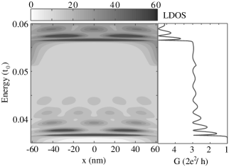
Figure 4: The local density states (LDOS) with the rectangular MB of 8T integrated over the y direction (in units of $t^{-1}_{0}$nm^-1), as a function of energy and $x$ in the zigzag GNR. The LDOS plot shows the localized states form inside the magnetic barrier. The position of the localized states in relation to the corresponding conductance.

In the zigzag GNR with a MB, the conductance steps also move towards higher energies and follow $N_{B}$ vs energy as $B$ increases, see Fig. 3(c), (d). This, as in the case of the armchair GNRs, simply reflects the magnetic field induced shifts of the GNR modes in the barrier region. Around $E=0$ , an energy interval exists in which only the lowest propagating state contributes to the conductance. This state evolves from the dispersionless edge state present in the zigzag GNRs at zero energy. The MB is thus able to reduce the number of current carrying states in certain energy intervals, e.g. between $E\approx 0.03t_{0}$ and $E\approx 0.037t_{0}$ for the MBs with a strengths of $8\,\mathrm{T}$. Note that for the zigzag GNR the conductance changes in steps of $2\times 2e^{2}/h$, whereas for the armchair GNR it changes in steps of $2e^{2}/h$. This reflects the difference in evolution of the subband structure of corresponding homogeneous armchair and zigzag GNRs, where the number of states at the given energy depends on the wire width $N$ and on whether the ribbon is metallic or insulating. (The conductance quantization for armchair and zigzag GNRs was discussed by Peres et al.).Peres2006a

In addition, as in the case of the armchair GNR, transmission resonances are observed for the rectangular MBs. These resonances are completely suppressed for the case of the smooth barriers. Both the frequency and the amplitude of the oscillations become higher as the strength of the MBs is increased (Fig. 3). Furthermore, the frequency decreases as the length of the MB is decreased (not shown). This behavior is similar to the conductance resonances in quantum point contacts with abrupt openings Maao1994 and originates from multiple reflections at the edges of the MB along the transport direction. The multiple reflections at the edges lead to the $\mathrm{{Fabry-P\acute{e}rot}}$ type oscillations, as can be seen in Fig. 4 for the case of a GNR with zigzag edges where the number of maxima in the LDOS along the transport direction changes by one for successive resonances. Similar to the case of a smooth quantum point contact Maao1994 , a gradual change of the magnetic field reduces the reflection probabilities and suppresses the resonances, resulting in smaller oscillation amplitudes.

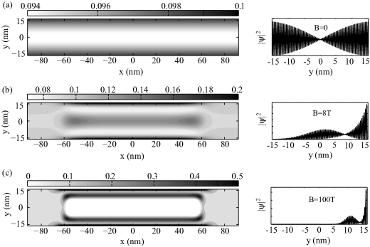
Figure 5: Spatial distributions of local density of states in the zigzag GNR with $N=151$ (left column) without a magnetic barrier (a), with a rectangular barrier of strength $B=8\,\mathrm{T}$ (b) and $B=100\,\mathrm{T}$ (c) extending from $x=-60\,\mathrm{nm}$ to $x=60\,\mathrm{nm}$. The gray scales (indicated by the bars on top) give the LDOS in units of $t^{-1}_{0}$nm^-2 . The Fermi energy is $E_{F}=0.01t_{0}$ corresponding to the case when only the lowest propagating state is occupied.The corresponding probability densities of the lowest Bloch state (in arbitrary units) in an infinite homogeneous wire are shown in the right column.

The dependence of the conductance on the magnetic barrier suggests that complete confinement by magnetic barriers is not possible due to the presence of the lowest propagating state, in stark contrast to the case of two-dimensional graphene sheets.Martino To shed more light on the influence of the MB on the lowest propagating state, we study the local density of state (LDOS) of the zigzag GNR in the energy interval where only the lowest propagating state is occupied, see Fig. 5. A rectangular MB strongly modifies the lowest propagating state in the transverse direction. The wave function patterns in the barrier region can be easily understood from analysis of the corresponding patterns of Bloch states in the homogeneous wire. The latter are shown in the right column of Fig. 5. The lowest propagating state in the absence of the MB (Fig. 5 (a)) extends across the whole GNR at this energy. At $B=8\,\mathrm{T}$, its probability density has a node at about $7\,\mathrm{nm}$ away from the edge, and a local maximum is formed close to the center of the GNR. As $B$ increases, this structure is pushed towards the edge of the GNR while its shape persists. A comparison of these patterns demonstrates that the wave function in the barrier region is directly related to the corresponding eigenstate of the homogeneous channel. Note that due to reflection on the barrier boundaries the edge state circulates inside the barrier region such that in this region $|\psi|^{2}$ has similar amplitude near the upper and lower edges of the wire. We note further that the rapid oscillations corresponding to the wave functions on the sites belonging to the A and B sublattices are averaged out in the grey-scale plots to the left.

The presence of this lowest propagating state apparently hampers the control of the carrier confinement in GNRs by MBs. It would thus be important to find a way to localize the lowest propagating state in gapless GNRs. There has been a lot of theoretical effort to explore a way to open a bandgap in metallic GNRs, such as application of uniaxial strain, boron doping, and introduction of a line of impurities Filho . To the best of our knowledge, no metallic behavior of GNRs with widths as studied here has been observed experimentally Han . It was pointed out that the major discrepancies between experiments and theory may arise from the assumptions of perfect GNRs with a well-defined type of edge used in most theoretical studies. Experimental observations reveal that edge disorder is very significant on natural graphite edges and etched GNRs. Theoretical studies have shown that the edge disorder dramatically affects the transport properties and may turn the metallic ribbons into semiconductors Querlioz . Since the edge disorder is usually present in realistic GNRs, we investigate the transport properties in such GNRs subjected to a MB.

Figure 6: The Fermi energy dependence of the conductance of defective graphene ribbons with and without the rectangular MB of strengths $8\,\mathrm{T}$. The edge defect concentration is 30%.

In Fig. 6 we show the conductance of a zigzag GNR with edge disorder with and without a MB as a function of Fermi energy. The edge defects are implemented by randomly removing 30 % of the atoms at the edges on both sides of the GNR, both inside and outside the magnetic barrier region. We first look at the conductance behavior in low energy regime. The characteristic feature is the appearance of conductance dips at the specific values of the Fermi energy. Similar dips are also found in GNRs with additional bonds attached to the edges Wakabayashi . As the concentration of edge defects increases, the dips become more prominent and more zero-conductance dips appear, and their position and structure changes as the defect configuration is varied (not shown). When the MB is activated, the position of some conductance dips, presumably those originating from defects underneath the MB, move in energy while their amplitude is suppressed. The effect of the magnetic field is therefore to delocalize the lowest propagating state which have been localized by the edge defects. These results suggest that a magnetic barrier can in fact be used to switch the conductance in a GNR, but the mechanism differs from that one to be expected for magnetic barriers in two-dimensional graphene. Activation of the MB is able to delocalize the lowest propagating state in GNRs with disorder, thereby switching the conductance from zero to one.

V Summary and conclusions

We have provided an extensive theoretical study of the transport through graphene nanoribbons under the influence of magnetic barriers. The magnetic barrier modifies the energy spectrum of the nanoribbon locally, which results in an energy shift of the conductance steps. In addition, multiple reflections along the transport direction between the entrance and the exit of the magnetic barrier generate $\mathrm{{Fabry-P\acute{e}rot}}$ resonances, the magnitude of which depends on the gradient of the magnetic field. These $\mathrm{{Fabry-P\acute{e}rot}}$ resonances are strongly suppressed in the case of magnetic barriers with smooth confinement. The lowest propagating state present in zigzag and metallic armchair GNRs is only weakly modified by magnetic barriers of realistic strengths. However, localization of the lowest propagating state by disorder can be lifted by a perpendicular magnetic field, which offers a concept for magnetic barrier induced conductance switching in GNRs with disordered edges.

In this paper we also present a novel method based on the Greens function technique for the calculation of the magnetosubband structure, Bloch states and magnetoconductance of the graphene nanoribbons in a perpendicular magnetic field. The non-trivial part of the method is the calculation of the surface Greens function $\Gamma$, which typically requires very time-consuming self-consistent calculations. We, however, introduced a novel way to calculate the surface Greens function that does not require self-consistent calculations, EPAPS and where $\Gamma$ is simply obtained from the solutions of the eigenequation of the dimension $2N\times 2N$ (with $N$ being the width of the nanoribbon). Utilization of this method obviously greatly facilitates computations, making the present method by far more efficient in comparison to the existing methods based on the self-consistent calculations of $\Gamma$. The programming codes are freely available in the AIP EPAPS electronic depository.EPAPS

Appendix A Hopping matrixes U

In this appendix we provide explicit expressions for hopping matrixes $U_{i,i^{\prime}}$, Eq. (11), for armchair and zigzag ribbons in the Landau gauge $\mathbf{A}=(-By,0)$. The numbering of slices and sites, $r=i,j,$ within a unit cell is given in Fig. (2), and the definition of the phases $\theta_{r,r+\Delta}=2\pi\phi_{r,r+\Delta}/\phi_{0}$ and the corresponding line integrals $\phi_{r,r+\Delta}$ are given by Eq. (4). In the expressions given below $y_{i,j}$ stands for the $y$-coordinate of the site ($i,j$).

A.0.1 Armchair graphene ribbon

$$\left(U_{1,0}\right)_{j,j^{\prime}}=-t_{0}\exp(i\theta_{0,j;1,j})\delta_{j,j^{\prime}};\ \ U_{0,1}=U_{1,0}^{+}$$ (35)

where $\phi_{0,j;1,j}=-By_{0,j}a;$

$$U_{2,1}=-t_{0}\begin{pmatrix}e^{i\theta_{1,1;2,1}}&e^{i\theta_{1,2;2,1}}&&&\\ &e^{i\theta_{1,2;2,2}}&\ddots&0&\\ &&\ddots&e^{i\theta_{1,N-2;2,N-1}}&\\ &0&&e^{i\theta_{1,N-1;2,N-1}}&e^{i\theta_{1,N-1;2,N}}\\ &&&&e^{i\theta_{1,N;2,N}}\end{pmatrix};\quad U_{1,2}=U_{2,1}^{+}$$ (36)

where $\phi_{1,j;2,j}=-\frac{B}{2}\left(y_{1,j}a+\frac{\sqrt{3}}{4}a^{2}\right),$ $\phi_{1,j+1;2,j}=-\frac{B}{2}\left(y_{1,j+1}a-\frac{\sqrt{3}}{4}a^{2}\right);$

$$\left(U_{3,2}\right)_{j,j^{\prime}}=-t_{0}\exp(i\theta_{2,j;3,j})\delta_{j,j^{\prime}};\ \ U_{2,3}=U_{3,2}^{+}$$ (37)

where $\phi_{2,j;3,j}=-By_{2,j}a;$

$$U_{4,3}=-t_{0}\begin{pmatrix}e^{i\theta_{3,1;4,1}}&&&&\\ e^{i\theta_{3,1;4,2}}&e^{i\theta_{3,2;4,2}}&&0&\\ &e^{i\theta_{3,2;4,3}}&\ddots&&\\ &0&\ddots&e^{i\theta_{3,N-1;4,N-1}}&\\ &&&e^{i\theta_{3,N-1;4,N}}&e^{i\theta_{3,N;4,N}}\end{pmatrix};\quad U_{3,4}=U_{4,3}^{+}$$ (38)

where $\phi_{3,j;4,j}=-\frac{B}{2}\left(y_{3,j}a-\frac{\sqrt{3}}{4}a^{2}\right),\;\phi_{3,j;4,j+1}=-\frac{B}{2}\left(y_{3,j}a+\frac{\sqrt{3}}{4}a^{2}\right);$ and, because of periodicity,

$$U_{5,4}=U_{1,0,}\;U_{4,5}=U_{0,1}.$$ (39)

A.0.2 Zigzag graphene ribbon

$$\left(U_{1,0}\right)_{j,j^{\prime}}=-t_{0}\exp(i\theta_{0,j;1,j})\delta_{j,j^{\prime}};\ \ U_{0,1}=U_{1,0}^{+},$$ (40)

where for odd $j$: $\phi_{0,j;1,j}=-\frac{\sqrt{3}}{2}B\left(y_{0,j}a+\frac{1}{4}a^{2}\right),$ and for even $j$: $\phi_{0,j;1,j}=-\frac{\sqrt{3}}{2}B\left(y_{0,j}a-\frac{1}{4}a^{2}\right)$

$$\left(U_{2,1}\right)_{j,j^{\prime}}=-t_{0}\exp(i\theta_{1,j;2,j})\delta_{j,j^{\prime}};\ \ U_{1,2}=U_{2,1}^{+},$$ (41)

where for odd $j$: $\phi_{1,j;2,j}=-\frac{\sqrt{3}}{2}B\left(y_{1,j}a-\frac{1}{4}a^{2}\right),$ and for even $j$: $\phi_{1,j;2,j}=-\frac{\sqrt{3}}{2}B\left(y_{1,j}a+\frac{1}{4}a^{2}\right);$ and, because of periodicity,

$$U_{3,2}=U_{1,0,}\;U_{2,3}=U_{0,1}.$$ (42)

References

- (1) For a review, see A. H. Castro Neto, F. Guinea, N. M. R. Peres, K. S. Novoselov, and A. K. Geim, arXiv:0709.1163v1, cond-mat.other.
- (2) Katsunori Wakabayashi, Mitsutaka Fujita, Hiroshi Ajiki, Manfred Sigrist, Phys. Rev. B 59, 8271 (1999).
- (3) M. I. Katsnelson, K. S. Novoselov and A. K. Geim, Nature Physics, 2, 620 (2006).
- (4) J. Milton Pereira, Jr. V. Mlinar, and F. M. Peeters, P. Vasilopoulos, Phys. Rev. B 74, 045424 (2006).
- (5) J. Tworzydlo, B. Trauzettel, M. Titov, A. Rycerz, and C. W. J. Beenakker, Phys. Rev. Lett. 96, 246802 (2006).
- (6) A. De Martino, L. Dell’Anna, and R. Egger, Phys. Rev. Lett. 98, 066802 (2007).
- (7) Yuanbo Zhang, Yan-Wen Tan, Horst L. Stormer, and Philip Kim, Nature (London) 438, 201 (2005).
- (8) K. S. Novoselov, A. K. Geim, S. V. Morozov, D. Jiang, M. I. Katsnelson, I. V. Grigorieva, S. V. Dubonos, and A. A. Firsov, Nature (London) 438, 197 (2005).
- (9) V. P. Gusynin and S. G. Sharapov, Phys. Rev. Lett. 95, 146801 (2005).
- (10) N. M. R. Peres, F. Guinea, and A. H. Castro Neto, Phys. Rev. B 73, 125411 (2006).
- (11) Wenjie Liang, Marc Bockrath, Dolores Bozovic, Jason H. Hafner, M. Tinkham, and Hongkun Park, Nature, 411, 665 (2001).
- (12) P. Jarillo-Herrero, S. Sapmaz, C. Dekker, L. P. Kouwenhoven, and H. van der Zant, Nature (London) 429, 389 (2004).
- (13) J. Nygard, D. H. Cobden, and P. E. Lindelof, Nature (London) 408, 342 (2000).
- (14) A. Javey, J. Guo, Q. Wang, M. Lundstrom, and H. Dai, Nature (London) 424, 654 (2003).
- (15) Mattias Hjort and Sven Stafström, Phys. Rev. B 63, 113406 (2001).
- (16) Xiaolin Li, Xinran Wang, Li Zhang, Sangwon Lee, Hongjie Dai, Science 319, 1229 (2008).
- (17) F. Muñoz-Rojas, D. Jacob, J. Fernández-Rossier, and J. J. Palacios, Phys. Rev. B 74, 195417 (2006).
- (18) F. M. Peeters and A. Matulis, Phys. Rev. B 48, 15166 (1993); A. Matulis, F. M. Peeters, and P. Vasilopoulos, Phys. Rev. Lett. 72, 1518 (1994).
- (19) Hengyi Xu, T. Heinzel, M. Evaldsson, S. Ihnatsenka, and I. V. Zozoulenko, Phys. Rev. B 75, 205301 (2007).
- (20) A. Majumdar, Phys. Rev. B 54, 11911 (1996)
- (21) F. Zhai and H. Q. Xu, Appl. Phys. Lett. 88, 032502 (2006).
- (22) R. Golizadeh-Mojarad, A. N. M. Zainuddin, G. Klimeck, S. Datta, arXiv:0801.1159v1 [cond-mat.mes-hall]
- (23) See EPAPS Document No. xx
- (24) R. Kubrak, A. Neumann, B. L. Gallagher, P. C. Main, M. Henini, C. H. Marrows, and B. J. Hickey, J. Appl. Phys. 87, 5986 (2000).
- (25) M. Cerchez, S. Hugger, T. Heinzel, and N. Schulz, Phys. Rev. B 75, 035341 (2007).
- (26) M. L. Leadbeater, C. L. Foden, J. H. Burroughes, M. Pepper, T. M. Burke, L. L. Wang, M. P. Grimshaw, and D. A. Ritchie, Phys. Rev. B 52, R8629 (1995).
- (27) S. Datta, Electronic Transport in Mesoscopic Systems, (Cambridge University Press, Cambridge, 1997).
- (28) D. K. Ferry and S. M. Goodnick, Transport in Nanostructures, (Cambridge University Press, Cambridge, 1997).
- (29) I. V. Zozoulenko, F. A. Maaø and E. H. Hauge, Phys. Rev. 53, 7975 (1996); ibid., 7987 (1996).
- (30) A. I. Rahachou and I. V. Zozoulenko, Phys. Rev. B 72, 155117 (2005).
- (31) S. Ihnatsenka and I. V. Zozoulenko, Phys. Rev. B 73, 075331 (2006).
- (32) N. M. R. Peres, A. H. Castro Neto, and F. Guinea, Phys. Rev. B 73, 195411 (2006).
- (33) T. Vanura, T. Ihn, S. Broderick, K. Ensslin, W. Wegscheider and M. Bichler, Phys. Rev. B 62, 5074 (2000).
- (34) F. A. Maaø I. V. Zozoulenko, and E. H. Hauge, Phys. Rev. B 50, 17320 (1994).
- (35) R. N. Costa Filho, G. A. Farias, and F. M. Peeters, Phys. Rev. B 76, 193409 (2007).
- (36) M. Y. Han, B. Ozyilmaz, Y. Zhang, and P. Kim, Phys. Rev. Lett. 98, 206805 (2007).
- (37) D. Querlioz, Y. Apertet, A. Valentin, K. Huet, A. Bournel, S. Galdin-Retailleau, and P. Dollfus, Appl. Phys. Lett. 92, 042108 (2008).
- (38) Katsunori Wakabayashi, Phys. Rev. B 64, 125428 (2001).