First-principles study of the optical properties of Mg_xTi_(1-x)H₂

Abstract

The optical and electronic properties of Mg-Ti hydrides are studied using first-principles density functional theory. Dielectric functions are calculated for Mg_xTi_(1-x)H₂ with compositions $x=0.5$, 0.75, and 0.875. The structure is that of fluorite TiH₂ where both Mg and Ti atoms reside at the Ti positions of the lattice. In order to assess the effect of randomness in the Mg and Ti occupations we consider both highly ordered structures, modeled with simple unit cells of minimal size, and models of random alloys. These are simulated by super cells containing up to 64 formula units ($Z=64$). All compositions and structural models turn out metallic, hence the dielectric functions contain interband and intraband free electron contributions. The former are calculated in the independent particle random phase approximation. The latter are modeled based upon the intraband plasma frequencies, which are also calculated from first-principles. Only for the models of the random alloys we obtain a black state, i.e. low reflection and transmission in the energy range from 1 to 6 eV.

I Introduction

Since the discovery of the switchable mirror YH_x by Huiberts et al.Huiberts et al. (1996) in 1996 several other metal hydride systems that behave as switchable mirrors have been discovered.Huiberts et al. (1996); van der Sluis et al. (1997); Richardson et al. (2001); Isidorsson et al. (2002); Lohstroh et al. (2004); Borsa et al. (2006). The metals are reflective, but after hydrogenation become semiconductors and hence in most cases become transparent. Especially when an alloy with high hydrogen mobility is used and when applied as thin films the optical switching can be fast, reversible and robust.Lohstroh et al. (2007)

Recently, meta-stable thin films composed of various ratios of magnesium and titanium have been shown to exhibit remarkable optical properties which could be especially useful for smart solar cell coatings and hydrogen sensor applications.Borsa et al. (2006); Slaman et al. (2007) In the dehydrogenated state the films are highly reflective. Upon hydrogenation they become black, i.e. have a low reflection and high absorption in the energy range of the solar spectrum. The structural and electronic characteristics of this black state are a topic of intensive research.Borsa et al. (2007); Er et al. (2007)

Obtaining structural data for these systems is difficult. Single crystals cannot be grown as the compounds are thermodynamically unstable. For a 7:1 ratio of magnesium to titanium Kyoi et al., using a sample prepared at high pressure, could determine the crystal structure.Kyoi et al. (2004) It is similar to the fluorite TiH₂ structure. Notten and co-workers (Refs. Niessen and Notten, 2005; Vermeulen et al., 2006a) and Borsa et al.Borsa et al. (2006, 2007) have shown that for higher titanium content ($x<0.8$) the structure is fluorite-like as well. At lower lower titanium concentrations a rutile ($\alpha$-MgH₂ like) structure is found. Interestingly, the kinetics of the hydrogen ab/desorption reactions are much faster in the fluorite structures than in the rutile structures.Vermeulen et al. (2006b) The equality of the molar volume of TiH₂ and Mg has been used to explain the structural stability of the meta-stable “phases”.Borsa et al. (2007) Calculations using density functional theory (DFT) find the same composition dependence of the relative stability of the rutile and fluorite structures.Er et al. (2007)

The origin of the “black state” is not understood. Its explanation is, of course, intimately related to the electronic structure of the hydride. In experiments, usually less than two hydrogen atoms per metal atom can be reversibly absorbed and desorbed.Borsa et al. (2007) Electrochemically 1.7 hydrogen atoms per metal atom can be stored reversibly.Vermeulen et al. (2006b) Moreover, the crystal structure of Mg₇TiH_x as determined by Kyoi et al.Kyoi et al. (2004) is estimated to contain 1.6 hydrogen atoms per metal atom. All this suggests that maximally two metal electrons per metal atom can be transferred to hydrogen.Borsa et al. (2007) Hence the Ti atoms remain in an open-shell configuration with at least two $d$-electrons left. The above reasoning has been confirmed by DFT calculations on crystalline Mg_xTi_(1-x)H₂ structures.Er et al. (2007) The calculated densities of states show predominant hydrogen-$s$ character below the Fermi level, which is typical for metal hydrides, and titanium-$d$ states at the Fermi level. These are likely to form metallic bands, so one expects Mg_xTi_1-xH₂ to be reflective instead of black. Moreover, experimental investigation of the electrical transport properties reveal high resistivity 1.32–1.9 m$\Omega$cm, with a logarithmic, hence non-metallic, temperature dependence.Borsa et al. (2007) In order to explain these results the formation of a so-called coherent crystal structure was proposed,Borsa et al. (2007) wherein regions of insulating MgH₂ and metallic TiH₂ coexist.

In an effort to advance the understanding of the black state, in this paper we report a computational study of the optical and electronic properties of Mg_xTi_(1-x)H₂ for $x=0.5$, 0.75 and 0.875. We employ both simple (i.e. minimal) unit cells and large super cells of the same compositions. The latter model random alloys wherein the Mg and Ti are distributed over the lattice sites of a TiH₂-like structure. Details of these models are presented in Ref. Er et al., 2007.

The dielectric functions consist of intra and interband contributions:

$$\varepsilon(\omega)=\varepsilon_{\rm inter}(\omega)+\varepsilon_{\rm intra}(\omega)~{}~{}.$$ (1)

These are calculated separately. For the interband contribution $\varepsilon_{\rm inter}$ we use first-principles DFT in the independent particle random phase approximation. Since the materials in question are metals, the intraband dielectric part $\varepsilon_{\rm intra}$ does not vanish. It is modeled from the plasma frequencies $\omega_{\textrm{p}}$, which are calculated from first-principles as well.

In Sec. II the technical details of the calculations are summarized. Sec. III contains a concise description of the structural models used. Results on the dielectric functions are presented in Sec. IV. Finally, in the discussion section (Sec. V) results are compared with experiment.Borsa et al. (2007)

II Computational methods

First-principles DFT calculations were carried out with the Vienna Ab initio Simulation Package (VASP),Kresse and Furthmüller (1996a, b); Kresse and Hafner (1993) using the projector augmented wave (PAW) method. Kresse and Joubert (1999); Blochl (1994) A plane wave basis set was used and periodic boundary conditions applied. The kinetic energy cutoff on the Kohn-Sham states was 312.5 eV. For the exchange-correlation functional we used the generalized gradient approximation (GGA).Perdew et al. (1992) Non-linear core corrections were applied.Louie et al. (1982)

The Brillouin zone integrations were performed using a Gaussian smearing method with a width of 0.1 eV.Blöchl et al. (1994). The $\bf k\rm$-point meshes were even grids containing $\Gamma$ so that the band extrema are typically included in the calculation of the dielectric functions. The convergence of the dielectric functions and intraband plasma frequencies with respect to the $\bf k\rm$-point meshes was tested by increasing the number of $\bf k\rm$-points for each system separately. A typical mesh spacing of about 0.01 Å^-1 was needed to obtain converged results.

The calculations of the complex interband dielectric functions, $\varepsilon_{\rm inter}(\omega)=\varepsilon_{\rm inter}^{(1)}(\omega)+i\varepsilon_{\rm inter}^{(2)}(\omega)$, were performed in the random phase independent particle approximation, i.e. taking into account only direct transitions from occupied to unoccupied Kohn-Sham orbitals. Local field effects were neglected. The imaginary part of the macroscopic dielectric function, $\varepsilon_{\rm intra}^{(2)}(\omega)$, than has the form:

$$\varepsilon_{\rm inter}^{(2)}(\mathbf{\hat{q}},\omega) = \frac{8\pi^{2}e^{2}}{V}\lim_{|\mathbf{q}|\to 0}\frac{1}{\left|\mathbf{q}\right|^{2}}\times$$

$$\sum_{\mathbf{k},v,c}\left|\left<u_{c,\mathbf{k}+\mathbf{q}}|u_{v,\mathbf{k}}\right>\right|^{2}\delta(\epsilon_{c,\mathbf{k}+\mathbf{q}}-\epsilon_{v,\mathbf{k}}-\hbar\omega)$$

where $\mathbf{\hat{q}}$ denotes the direction of $\mathbf{q}$ and $v,\mathbf{k}+\mathbf{q}$ and $c,\mathbf{k}$ label single particle states that are occupied and unoccupied in the ground state, respectively. $\epsilon$, $u$ are the single particle energies and the translationally invariant parts of the wave functions. $V$ is the volume of the unit cell. The real part, $\varepsilon_{\rm inter}^{(1)}(\omega)$, is obtained via a Kramers-Kronig transform. Further details can be found in Ref. Gajdoš et al., 2006.

Most optical data on hydrides are obtained from micro- and nano-crystalline samples whose crystallites have a significant spread in orientation. Therefore the most relevant quantity is the directionally averaged dielectric function, i.e. $\varepsilon_{\rm inter}^{(2)}(\omega)$ averaged over $\mathbf{\hat{q}}$.

The intraband dielectric function, $\varepsilon_{\rm intra}(\omega)=\varepsilon_{\rm intra}^{(1)}(\omega)+i\varepsilon_{\rm intra}^{(2)}(\omega)$, is calculated from the free electron plasma frequency $\omega_{\textrm{p}}$:

$$\varepsilon_{\rm intra}^{(1)}(\omega) = 1-\frac{\omega^{2}_{\textrm{p}}}{\omega^{2}+\gamma^{2}}$$ (3)

$$\varepsilon_{\rm intra}^{(2)}(\omega) = \frac{\gamma\omega^{2}_{\textrm{p}}}{\omega^{3}+\omega\gamma^{2}}$$ (4)

where an inverse lifetime, $\gamma=0.01$ eV, is used. For $\gamma=0$ the reflection would be perfect up to the plasma frequency and zero beyond. Finite values of $\gamma$ decrease the reflection below $\omega_{\textrm{p}}$ and smoothen the reflection edge at $\omega_{\textrm{p}}$. For metals $\gamma$ values are in the order of 0.1 eV. By using a small value the influence of the interband part is emphasized. Calculating $\gamma$ from first principles obviously goes beyond DFT. For three values of $\gamma$ the free electron $\varepsilon_{\rm intra}$ is plotted in Fig. 1.

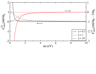
Figure 1: (Color online) Dielectric functions of a free electron gas according to equation 3.

The plasma frequency $\omega_{\textrm{p}}$ is calculated as an integral over the Fermi surface according to:

$$\omega^{2}_{\textrm{p}(\alpha\beta)}=\frac{4\pi e^{2}}{V\hbar^{2}}\sum_{n,\mathbf{k}}2g_{\mathbf{k}}\frac{\partial f(\epsilon_{n\mathbf{k}})}{\partial\epsilon}\left(\mathbf{e}_{\alpha}\frac{\partial\epsilon_{n\mathbf{k}}}{\partial\mathbf{k}}\right)\left(\mathbf{e}_{\beta}\frac{\partial\epsilon_{n\mathbf{k}}}{\partial\mathbf{k}}\right)$$ (5)

with $g_{\mathbf{k}}$ the weight factors, and $f(\epsilon_{n\mathbf{k}})$ the occupation function. Again we use directionally averaged values. Further details on the calculation of the plasma frequency can be found in Ref. Harl et al., 2007.

Finally the optical constants, the refraction index, $n$, and the extinction coefficient, $\kappa$, and the absorption, $A$, reflection, $R$, and transmission, $T$, are calculated using the standard expressions:

$$n = \frac{1}{\sqrt{2}}\sqrt{\varepsilon^{(1)}+\sqrt{{\left(\varepsilon^{(1)}\right)}^{2}+\left(\varepsilon^{(2)}\right)^{2}}}$$ (6)

$$\kappa = \frac{1}{\sqrt{2}}\sqrt{-\varepsilon^{(1)}+\sqrt{\left(\varepsilon^{(1)}\right)^{2}+\left(\varepsilon^{(2)}\right)^{2}}}$$ (7)

$$A = 1-\exp(-\kappa\omega d/c)$$ (8)

$$R = \frac{(n-1)^{2}+\kappa^{2}}{(n+1)^{2}+\kappa^{2}}$$ (9)

$$T = (1-R)(1-A),$$ (10)

with $\varepsilon^{(1)}$ and $\varepsilon^{(2)}$ the real and imaginary part of $\varepsilon$, $d$ the slab thickness and $c$ the speed of light in vacuum. The reflection and transmission spectra are constructed to simulate the substrate/Mg_xTi_(1-x)H₂/palladium setup as was used in the experiments by Borsa et al.Borsa et al. (2006, 2007) All internal reflections and absorptions in the three layer system are taken into account.

III Structures

The calculation of the dielectric functions is performed using the crystal structures developed in Ref. Er et al., 2007. A brief summary of compositions and cell parameters is given in Table 1. In short they were constructed in the following way.

In the case of $x=0.875$ the simple cell is just the optimized experimental cell with composition Mg₂₈Ti₄H₆₄. For $x=0.5$ and 0.75, two and three atoms, respectively, out of the four titanium atoms in the conventional fcc TiH₂ cell were replaced by magnesium. Thus the unit cells have compositions Mg₂Ti₂H₈ and Mg₃TiH₈ respectively.

To simulate the random alloys super cells are used. These are also based on the fluorite Ti₄H₈ ($Z=1$) building block. For $x=0.5$ and 0.75 $2\times 2\times 2$ super cells were constructed and for $x=0.875$ a $2\times 1\times 1$ super cell. Again Ti were replaced by Mg, but now such as to approximate random alloys most efficiently (see Ref. Er et al., 2007 for details).

For all the models constructed the positional and cell parameters were relaxed. The cells remain close to cubic, see Table 1. The angles between the crystal axes are close to 90^∘, except for the $x=0.75$ and 0.875 super cells where there is a small deviation.

Table 1: Number of formula units (Z), lattice parameters (Å) and shortest Ti–Ti interatomic distances (Å). The first row for each composition contains the data of the simple cell and the second of the super cell.

x	Z	a	b	c	Ti–Ti
0.5	4	4.72	4.72	4.65	3.16
	32	9.08	9.03	9.09	3.15
0.75	4	4.62	4.62	4.62	4.62
	32	9.29	9.30	9.27	3.13
0.875	32	9.36	9.36	9.36	6.62
	64	18.75	9.42	9.73	3.08

IV Dielectric functions

IV.1 Interband dielectric functions

Figures 2 and 3 show the calculated imaginary parts of the interband dielectric functions in the simple and super cells respectively. In general the dielectric functions exhibit a peak at low energy, below 2 eV, followed by a relatively flat tail. In the super cells the dielectric functions have higher peaks and flatter tails. An exception is the dielectric function of the $x=0.875$ super cell. It does not have a peak at low energy.

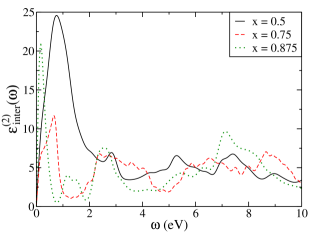
Figure 2: (Color online) Imaginary parts of the interband dielectric functions of Mg_xTi_(1-x)H₂ in the primitive cells.

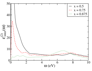
Figure 3: (Color online) Imaginary parts of the interband dielectric functions of Mg_xTi_(1-x)H₂ in the super cells. For $x=0.5$ the dielectric function peaks to a value of 130.

To understand the main features of the dielectric functions we study the densities of states (DOS’, Fig. 4). Below the Fermi level the DOS’ have an approximately triangular shape with a predominant hydrogen-$s$ and magnesium-$s$ and $p$ character. At the Fermi level the DOS’ are dominated by titanium-$d$ states. Above the Fermi level the DOS’ have a mixed character of hydrogen-$s$ and $p$, magnesium-$s$ and $p$ and titanium-$d$. As an illustration the angular momentum projected partial DOS’ of the simple cell with $x=0.75$ is shown in Fig. 5.

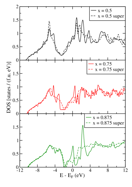
Figure 4: (Color online) Electronic densities of state of the simple and super cells for the three compositions of Mg_xTi_(1-x)H₂. The zero of energy is taken at the Fermi level.

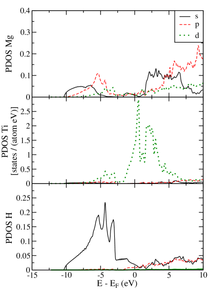
Figure 5: (Color online) Angular momentum projected partial densities of states (PDOS) [states/(atom eV)] of Mg_0.75Ti_0.25H₂ in the simple unit cell. The zero of energy is at the Fermi level. The PDOS’ are calculated in spheres with radii of 1.3, 1.3 and 0.8 Å for Mg, Ti an H respectively.

The electron density is localized at both the hydrogen and titanium atoms. This is illustrated in Figure 6, where the electron localization function (Ref. Silvi and Savin, 1994) is plotted, also for the simple cell Mg_0.75Ti_0.25H₂. At the titanium atoms the only available states are of $d$-character. Since $d-d$ transitions are very weak the main contribution to the dielectric function is from $s-p$ transitions on the hydrogen atoms.

Figure 6: (Color online) Electron localization function of Mg_0.75Ti_0.25H₂ in the simple unit cell. The Ti atoms are at the corners, the Mg atoms at the face centers and the H atom (small) are inside the cell. The electron localization function is plotted on a (110) cut-plane. Localization at the H and Ti atoms is evident.

In first order the imaginary part of the dielectric function can be described as the joint density of states (JDOS) divided by $\omega^{2}$. The hydrogen DOS has a dip near the Fermi energy. It increases when moving away from the Fermi energy, both to lower and higher energies. This causes the JDOS at the hydrogen atoms to increase more than linearly (in the region from 0 to about 8 eV). When divided by $\omega^{2}$ this increase is rather effectively compensated. Hence the dielectric function does not vary much in the interval from 2 to 8 eV. This reasoning applies for all titanium concentrations that we considered. In the super cells the averaging over the various hydrogen DOS’ gives rise to a further leveling out of the dielectric functions. Of course vibrational effects, that are lacking in our 0 K calculation, will even further smoothen the dielectric functions.

The peaks at the lower end of the energy range do arise from d-d transitions on the Ti atoms. Although their oscillator strength is small, division by $\omega^{2}$ causes them to stand out nevertheless. For $x=0.875$ the Ti DOS at $E_{\rm Fermi}$ is strongly suppressed in the super cell (see Fig. 4). This correlates with the absence of the peak in $\epsilon_{\rm inter}^{(2)}$ for the super cell at this composition (Figs. 2, 3). At the other two compositions, we see no clear correlation between difference in DOS and peak shape (comparing simple and super cells). The higher peaks in the DOS in the super cells can be understood when we realize that the effective “back folding” of the d bands and their mutual interactions (caused by the randomization) results in a flattening of the bands. Some of these bands will be very close to $E_{\rm Fermi}$ and their transitions will thus be “boosted”, both by the flatness of the bands and the small transition energy. This discussion anticipates the discussion in the next section.

IV.2 Intraband plasma frequencies

The intraband plasma frequencies, which have been calculated according to Equation 5, are listed in Table 2. The squared plasma frequencies from the super cell calculations are between one and two orders of magnitude smaller than those of the simple cells. Therefore the edge on the free carrier reflectively occurs at considerably lower energies in the random alloys. In our models the maximum $\omega_{\rm p}$ is 1.1 eV. This is, however, for only one realization of a random model at $x=0.5$ and it is well conceivable that calculations on large models could yield even lower $\omega_{\rm p}$. For the simple cells, the plasma frequencies are approximately 3 eV, hence these systems are highly reflecting for $\omega<3$ eV.

Table 2: Squared plasma frequencies, $\omega_{\textrm{p}}^{2}$ (eV²), from intraband transitions.

	simple cell	super cell
$x=0.5$	10.7	1.3
$x=0.75$	12.8	0.4
$x=0.875$	8.6	0.1

Eq. 5 is a good starting point for a discussion of the trends across Table 2. It basically states that the squared plasma frequency is proportional to the product of the electron density and the square of the slope of the energy bands, both calculated at the Fermi level. In the super cells $\omega_{\textrm{p}}^{2}$ clearly follows the density of states (see, Fig. 4) as a lower concentration of titanium means a lower amount of free electrons. In the simple cells this trend is not obvious. Subtle changes in the shape of the DOS, i.e. bandstructure effects, make for less changes in the electron density at the Fermi level. Consistently the plasma frequency shows little variation. This, however, does not imply that small changes in the slope of the energy bands do not play an equally important role here.

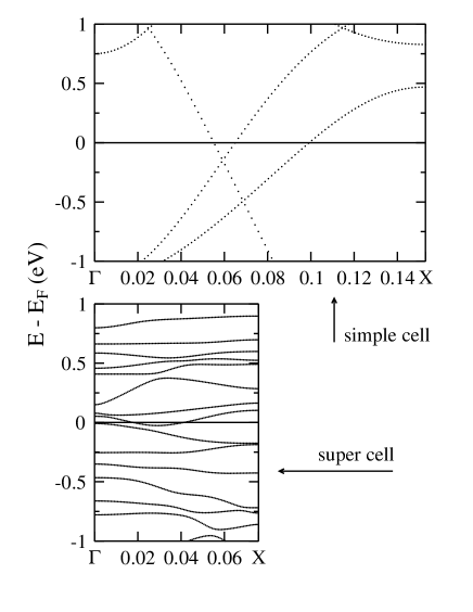
Figure 7: Electronic energy band structure of Mg_0.75Ti_0.25H₂ in the simple and super cell along the $\Gamma$–X direction.

The difference between the simple and super cells of the same composition is explained by a decrease in energy band slope. The DOS’ at the Fermi level are of comparable size, at least for compositions with $x=0.5$ and $x=0.75$. This clearly points to the change in $\partial\epsilon_{n\bf k}/\partial\epsilon_{\bf k}$ as the cause of the significant decrease of $\omega_{\rm p}$. This is corroborated by inspection of the band structure, that is plotted in Fig. 7 for Mg_0.75Ti_0.25H₂ for both the simple and super cell. We see that the bandstructure of the supercell cannot be understood as a simple back-folding of the bands. The randomness in the structure has induced many interactions between the $d$-bands, leading to a dramatic reduction of their slopes. Going to even larger super cells, the effect may become even stronger, and the free carrier reflection concomitantly reduced. Such a calculation goes beyond the present study. It may require a different formalism as the reciprocal space description of Eq. 5 is bound to break down for truly random systems.

Interestingly, the flatness of the energy bands also makes that the effective mass of the “free” electrons is rather high. This goes some way to explain the rather high resistivity measured for these systems. The “flat bands” also point to a possible localization of carriers.

For $x=0.875$ the reduction of $\omega_{\textrm{p}}^{2}$ cannot be understood as a reduction of only $\partial\epsilon_{n\bf k}/\partial{\bf k}$. From Fig. 4 a substantial reduction of the DOS at $E_{\rm Fermi}$ is evident. Hence reduction of $\omega_{\textrm{p}}^{2}$ is much stronger than for $x=0.5$ and $x=0.75$.

To obtain the dielectric functions of the materials we just add the interband part of Sect. IV.1 and intraband parts obtained from $\omega_{\textrm{p}}$ according to Eq. 1. It was already noted above that the impact on the reflection in the visible range will be substantial for the simple cells. The values of $\omega_{\textrm{p}}^{2}$ in the super cells are low enough to only induce minor corrections to the interband dielectric function. The implications of the corrections will be discussed in the next Section.

V Discussion

The calculations on the random alloy super cells clearly demonstrate that breaking of the short range order results in two important effects: (a) The interband dielectric function is smoothened and (b) the plasma frequency is lowered. The first translates in smoother reflection and transmission spectra for the super cells. The second results in a lower reflection edge. The simple cells have almost full reflection up to 1–2 eV whereas in the super cells full reflection only occurs below $\sim$0.3 eV.

Figure 8 shows the calculated reflection and transmission of a film simulating closely the experimental setup as used by Borsa et al.Borsa et al. (2007) The simulated film consists of 10 nm Paladium / 200 nm Mg_xTi_(1-x)H₂ / $(k=0)$ quartz substrate layers, were we use the $\varepsilon(\omega)$ calculated in the super cells for the Mg_xTi_(1-x)H₂ layer. The plotted range is that of a Perkin Elmer Lambda 900 diffraction spectrometer. For comparison; visible light lies in the range of 1.65–3.26 eV. The general features and trends as a function of Ti content in both reflection and transmission are in agreement with the trends observed in the experiments.Borsa et al. (2007) Indeed the reflection is low and our calculations describe a “black state”. With decreasing Ti content the reflection decreases and the transmission increases.

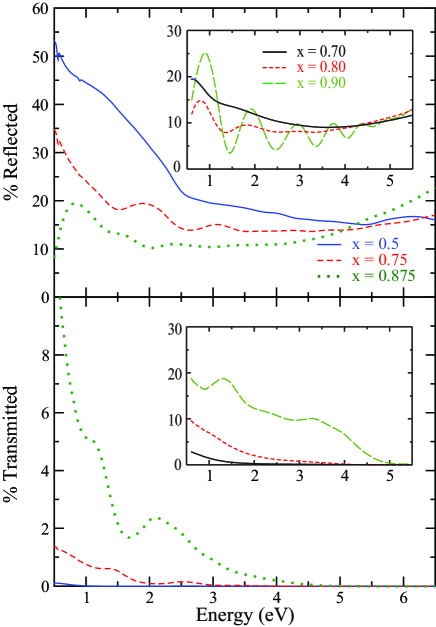
Figure 8: (Color online) Reflection and transmission of a 10 nm Paladium / 200 nm Mg_xTi_(1-x)H₂ / $(k=0)$ quartz substrate film. For the dielectric function of Mg_xTi_(1-x)H₂ the results for the supercell, including inter and intraband contributions, are used. The inset shows experimental results from Ref. Borsa et al., 2007, reproduced with permission, copyright American Physical Society (2007).

Since experiments were performed on magnesium/titanium ratios $x=0.7$, 0.8, and 0.9, that would have required very large super cells, a detailed comparison can only be made partially. Interpolating between the experimental values for 0.7 and 0.8 we can make a reasonable comparison with the calculated results for $x=0.75$. The experimental reflection lies about 5 %Pt. lower than the calculated one but the shape of the curve is very similar. The experimental transmission drops from 6.5%–0% in the range from 0.5–3 eV, it hence lies about a factor 3 higher than the calculated one. The shapes of the transmission curves, however shows good agreement.

Comparing the calculated values for $x=0.875$ to the experimental results for $x=0.9$ we again see somewhat lower values for the experimental reflection. Furthermore, the slight oscillation seen in the calculated spectrum, caused by interference, is much stronger in the experimental spectrum. The main difference in the transmission lies in the energy range below 1 eV where the calculated transmission is much larger than the experimental values. This difference could point to an underestimation of the $\omega_{\textrm{p}}^{2}$ in the super cell $x=0.875$ calculation.

From the correspondence between the experimental and calculated optical spectra we conclude that the “black state” can already be explained from moderate-size randomized super cells. Put into other words: randomized models containing only 32 to 64 formula units allow for a breaking of the order on a length-scale such as to lower the reflection edge and smoothen the spectra. This does not necessarily imply that a randomization at larger length scales, with a concomitant increase of the short range order, e.g. in the coherent crystal picture proposed by Borsa et al.Borsa et al. (2007), would be inconsistent with experiment. Indeed, the coherent crystal model is supported by various observations, e.g. the large positive enthalpy of mixing of Ti and Mg. Moreover, for $x=0.875$ our modeling seems to underestimate $\omega_{\rm p}$, suggesting that the short range disorder may have disrupted the band dispersion to much. A full first-principles study of necessarily larger models with more short range order is beyond present computational capabilities. Such a study is desirable. However, with the present randomized models we can capture most of the essential physics of Mg_xTi_1-xH₂.