Microscale fluid flow induced by thermoviscous expansion along a traveling wave

Abstract

The thermal expansion of a fluid combined with a temperature-dependent viscosity introduces nonlinearities in the Navier-Stokes equations unrelated to the convective momentum current. The couplings generate the possibility for net fluid flow at the microscale controlled by external heating. This novel thermo-mechanical effect is investigated for a thin fluid chamber by a numerical solution of the Navier-Stokes equations and analytically by a perturbation expansion. A demonstration experiment confirms the basic mechanism and quantitatively validates our theoretical analysis.

Spatial confinement of a liquid changes its flow behavior markedly, since the importance of surface forces relative to the volume forces increases as the confinement becomes smaller. Recently, flow at the scale of millimeters and below has attracted significant attention, stimulated by the rapid advances to manipulate and to control small-scale devices Stone et al. (2006); Whitesides (2006); Squireset al. (2005); Thorsenet al. (2002). Since microfluidic flow often is essentially at zero Reynolds number, viscous drag overwhelms the inertial effects of the fluid giving rise to peculiar flow behavior Happel et al. (1983); Batchelor (1977). In particular, heat conduction becomes quite efficient, since the thermal diffusivity $\kappa=k/\rho c_{p}$, with $k$ the thermal conductivity and $\rho c_{p}$ the volumetric heat capacity, implies thermal relaxation times $D^{2}/\pi^{2}\kappa$ of the order of $0.1\mbox{ms}$ for water confined by walls separated by $D=10$ µm. Usually, this strong thermal coupling gives rise to a uniform temperature and all physical processes are isothermal. Since pressure effects upon density are negligible if the velocities are small with respect to the speed of sound, fluid flow is essentially "dynamically incompressible" Batchelor (1967), i.e. the velocity field is solenoidal, $\mbox{div }\vec{v}=0$.

Recently, it has been noted by Yariv et al. (2006) that for the case of unsteady heating this is no longer the case and one can in principle generate a non-solenoidal flow. A transient fluid flow emerges due to a thermal expansion of the fluid as a reaction to the heating in combination with the thermal diffusion.

In this Letter we propose a novel mechanism to generate net flow in a thin fluid chamber, i.e. a viscous liquid confined between two plates separated by a distance of the order of a few micrometers. The driving of the fluid flow is provided by imposing a traveling temperature wave. We show analytically within a thin-film approximation that such unsteady heating leads to net fluid flow. Then we corroborate our analytic approach by a finite-element calculation. Last we provide first experimental evidence that there is indeed net flow and that the fundamental dependences have been correctly identified.

The basic mechanism may be summarized as follows: Due to thermal expansion of the liquid the motion of the heating results in a pressure modulation. The pressure gradients induce a potential flow which, however, does not lead to net fluid flow. Yet, the temperature dependence of the shear viscosity gives rise to a small net mass transport typically opposite to the motion of the heat source. The flow velocity is then proportional to the thermal expansion coefficient of the fluid, $\alpha=\rho_{0}^{-1}(\partial\rho/\partial T)$ as well as to the thermal viscosity coefficient $\beta=-\eta_{0}^{-1}(\partial\eta/\partial T)$.

The geometry under consideration consists of a thin chamber of height $D$ and a much larger lateral extension. There is a natural small parameter $\epsilon=D/L\ll 1$, where $L$ is a typical length scale in the lateral direction. Since the film is thin one expects the Navier-Stokes equations to be dominated only by a few terms. To identify the relevant contributions dimensionless quantities are introduced as $t=Tt^{*},v_{i}=Uv_{i}^{*},v_{i}=vv_{\perp}^{*},x_{i}=Lx_{i}^{*},x_{\perp}=Dx_{\perp}^{*},p=Pp^{*}$. Lateral directions are labeled by a latin index $i\in\{x,y\}$, whereas the vertical direction is indicated by the subscript $\perp$. To keep all terms in the mass conservation law the scales are chosen as $v=\epsilon U,T=L/U$, and consequently the fluid flow is essentially in-plane. To balance the leading order term in the momentum conservation law the pressure scale has to be chosen as $P=\eta_{0}U/(\epsilon^{2}L)$. Momentum transport via convective processes may be ignored from the very beginning since the Reynolds number is small, $\mbox{\sl Re}=\rho_{0}UL/\eta_{0}\ll 1$ . Then the mass conservation law and the momentum balance in perpendicular and lateral direction read to leading order in a thin-film approximation, see e.g. O’Brien et al. (2006); Oron et al. (1997); Leal (1992) (restoring units)

$$\partial_{t}\rho+\nabla_{\perp}(\rho v_{\perp})+\nabla_{i}(\rho v_{i}) = 0\,,$$ (1a)

$$\nabla_{\perp}p = 0\,,$$ (1b)

$$\nabla_{\perp}[\eta\nabla_{\perp}v_{i}]+\nabla_{i}p = 0\,.$$ (1c)

As a consequence of the thin film geometry, (i) bulk viscous processes do not contribute to the leading order equations, (ii) the pressure is homogeneous in the perpendicular direction, (iii) lateral pressure gradients drive the lateral fluid flow. Note that the divergence of the velocity field is irrelevant for the momentum balance but plays a crucial role in the mass conservation law.

The coupling to the temperature enters the equations via the expansion of the fluid as well as by the temperature dependence of the shear viscosity. For the problem at hand it is appropriate to neglect the mechanical compressibility of the fluid and to expand the equation of state to first order in the temperature field, $\rho=\rho_{0}(1-\alpha\delta T)$, where $\delta T$ is the local temperature change and $\alpha=-(\partial\ln\rho/\partial T)_{p}$ the thermal expansion coefficient at the reference state $(\rho_{0},T_{0})$. The density field then is eliminated from the equations of motion in favor of the temperature field $\delta T$. A second ingredient for the theoretical model is to include the variation of the shear viscosity with temperature. Introducing the thermal viscosity coefficient $\beta=-(\partial\ln\eta/\partial T)_{p}$, the coupling reads $\eta=\eta_{0}(1-\beta\delta T)$ to first order.

In the case of considerable thermal coupling to the walls the temperature field approximately reflects the profile of the heat source and then the temperature is uniform perpendicularly to the walls. The in-plane variations of the temperature field occur on scales $\lambda,b\gg D$, where $\lambda$ denotes the wavelength and $b$ the typical lateral extension of the heating. Consequently, the spatial dependence of the density and the shear viscosity is only in-plane as it is inherited from the temperature profile. With this additional assumption, the in-plane momentum balance equation, Eq. (1c), is readily integrated for no-slip boundary conditions at the walls

$$v_{i}=-\frac{1}{2\eta}z(D-z)\nabla_{i}p\,,$$ (2)

i.e. the velocity profile corresponds to Poiseuille flow.

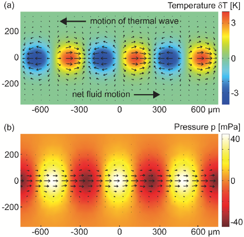
Figure 1: (color online) Finite element solution for a temperature wave in the comoving frame. (a) The temperature profile is indicated by the color scale and the arrows refer to the induced velocity flow. (b) The corresponding pressure modulation (color scale) and the solenoidal component of the flow.

Since the spatial dependence of the velocity profiles perpendicular to the wall is known, one may project the three-dimensional problem to the two-dimensional plane by averaging over the vertical $z$-direction,

$$\bar{v}_{i}=\frac{1}{D}\int_{0}^{D}v_{i}\mathrm{d}z=-\frac{D^{2}}{12\eta}\nabla_{i}p\,.$$ (3)

Because the density is assumed to vary only in the lateral direction, the mass conservation law, Eq. (1a), can be directly averaged over the perpendicular direction, $\partial_{t}\rho+\nabla_{i}(\rho\bar{v}_{i})=0$, without introducing new terms. The pumping process becomes stationary in the frame of reference comoving with the heat wave, i.e. substituting $\bar{v}_{x}\mapsto\bar{v}_{x}-u$, where $u$ denotes the velocity of the heat wave. Then in the comoving frame the averaged mass conservation law yields

$$-u\nabla_{x}\rho+\rho\nabla_{i}\bar{v}_{i}=-\bar{v}_{i}\nabla_{i}\rho\,.$$ (4)

Here the velocities $\bar{v}_{i}$ are small quantities, typically $\bar{v}_{i}\ll u$. From the closed set of equations, Eqs. (3) and (4), the fluid velocity can be calculated. The temperature profile in the comoving frame enters Eq. (4) in the form of density gradients, $\nabla_{i}\rho=-\alpha\rho_{0}\nabla_{i}\delta T$ and Eq. (3) via the temperature dependent viscosity. The net flow emerges only if the thermal viscosity coefficient $\beta$ is non-vanishing. For a temperature-independent viscosity the pressure acts as a velocity potential, Eq. (3), and averaging along the direction of the wave propagation yields a vanishing net flow.

We exemplify the flow profiles for the case of a gaussian temperature wave $\delta T(\vec{r})=\delta T_{0}\cos(kx)\,\text{e}^{-y^{2}/2b^{2}}$, obtained by a numerical solution of Eqs. (3) and (4) using the Femlab®3.1 software package by Comsol. We have used a wavelength $\lambda=2\pi/k=50$ µm, a lateral width $b=7$ µm of the gaussian modulation, a temperature amplitude of $\delta T_{0}=3.8\,\text{K}$, and a thermal wave velocity $u=100$ mm/s. The parameters for $\alpha=3.0\cdot 10^{-4}\,\text{K}^{-1}$, $\beta=0.022\,\text{K}^{-1}$ correspond to water at ambient temperature. The parameters have been chosen such that the temperature modulation appears approximately as a train of circular heated areas mimicking the demonstration experiment below. The regions where the temperature gradient is maximal (minimal) act as sources (sinks) for the velocity field, giving rise to a locally dipolar pattern of the fluid flow, see Fig. 1(a). Careful inspection reveals that the velocities in the heated regions are bigger than in the colder ones. The pressure profile is shifted by a quarter of a wavelength reflecting the local expansion of the fluid, Fig. 1(b). The solenoidal part of the velocity field has been obtained as the difference of two Femlab calculations for thermal viscosity coefficients $\beta\neq 0$ and $\beta=0$. Close to the center of the wave this contribution is directed opposite to the thermal wave velocity with an average pump velocity $v_{\text{fl}}^{\text{FEM}}=2.88$ µm/s at the center of the thermal wave, whereas far away from the heating there is a characteristic backflow. The pressures induced by the pumping are below $10^{-6}$ bar (Figure 1b). The pressure limitations of the glass chamber used are estimated to 10 bar by a finite element calculation. However, the pressure induced by the pumping increases with the viscosity of the fluid and eventually will stall the pump motion since thermal expansion will deform only the chamber walls instead of triggering fluid motion. So we expect to equally pump fluids with viscosities $10^{7}$ fold higher than water.

To gain further insight, we develop a perturbative analytical solution for the fluid flow appropriate for small temperature changes. Formally, the expansion is performed in the small parameters $\alpha$ and $\beta$, and we shall show that net fluid flow first occurs at ${\cal O}(\alpha\cdot\beta)$. The quiescent fluid $v_{i}\equiv 0,p=p_{0}$ solves the governing equations to zeroth order in $\alpha,\beta$, i.e. if all couplings to the temperature field are ignored. To leading order in $\alpha$, the term on the r.h.s. of Eq. (4) is of second order and may be ignored. Similarly,  (3) is expanded to first order in the temperature change

$$\bar{v}_{i}=-\frac{D^{2}}{12\eta_{0}}(\nabla_{i}p)(1+\beta\delta T)\,.$$ (5)

Already at this point one concludes that to order ${\cal O}(\beta^{0})$ the velocity corresponds to potential flow only, hence no net pumping arises to that order. The leading order to the pump velocity is then expected to be of order ${\cal O}(\alpha\beta)$. To identify the net fluid motion it is favorable to introduce the velocity potential, $\chi$, and the stream function,$\psi$, via $\bar{v}_{x}=\nabla_{x}\chi+\nabla_{y}\psi,\bar{v}_{y}=\nabla_{y}\chi-\nabla_{x}\psi$. From Eq. (5) one infers that the leading term corresponds to pure gradient flow, i.e. $\chi=-(D^{2}/12\eta_{0})p$, where $\chi(\vec{r})$ denotes the velocity potential and $\vec{r}=(x,y)$. To the required order $\chi$ is determined by combining Eqs. (4)

$$\nabla^{2}\chi(\vec{r})=-\alpha u\nabla_{x}\delta T(\vec{r})+{\cal O}(\alpha^{2})\,.$$ (6)

Once the velocity potential is determined, the stream function is calculated by extracting from $\beta\delta T(\vec{r})\nabla_{i}\chi(\vec{r})$ its solenoidal component. By Helmholtz’s decomposition theorem, the stream function satisfies a Poisson equation

$$-\nabla^{2}\psi=\nabla_{x}(\beta\delta T\nabla_{y}\chi)-\nabla_{y}(\beta\delta T\nabla_{x}\chi)\,.$$ (7)

The lowest order contribution to the stream function is thus proportional to $\alpha\cdot\beta$, which also sets the overall scale of the thermo-mechanical effect. Furthermore one infers from Eq. (7), that a strictly one-dimensional temperature modulation does not give rise to solenoidal flow. The remaining task is to solve the set of Poisson equations, which can be easily implemented by numerical methods. To determine the average flow for a travelling periodic temperature wave train of wavelength $\lambda$, it is actually sufficient to know the velocity potential,

$$v_{\text{fl}}(y) \equiv \frac{1}{\lambda}\int_{0}^{\lambda}\!\!\mathrm{d}x\,\bar{v}_{x}(\vec{r})=-\frac{1}{\lambda}\int_{0}^{\lambda}\!\!\mathrm{d}x\,\chi(\vec{r})\beta\nabla_{x}\delta T(\vec{r})\,,$$

where the last relation follows from the representation, Eq. (5) and an integration by parts.

To illustrate the physics we consider a gaussian temperature wave $\delta T(\vec{r})=\delta T_{0}\cos(kx)\text{e}^{-y^{2}/2b^{2}}$, where $b$ characterizes the lateral width of the wave train. The Poisson equation, Eq. (6), can be solved exactly in terms of error functions Kraus (2007), however, it is instructive to construct an approximate solution for wide waves, $kb\gg 1$. Then the problem is effectively one-dimensional, and $\chi$ depends on the lateral coordinate $y$ only parametrically. One readily calculates $\chi=-u\alpha\delta T_{0}\sin(kx)\text{e}^{-y^{2}/2b^{2}}/k$, implying a net fluid motion

$$v_{\text{fl}}(y)=-u\alpha\beta(\delta T_{0})^{2}\exp(-y^{2}/b^{2})/2\,,$$ (9)

typically opposite to the motion of the traveling temperature wave. Since by assumption the changes in the density and the viscosity are small, the net fluid motion is much slower than the velocity of the temperature wave, $v_{\text{fl}}\ll u$.

We have confirmed the predicted fluid movement in a demonstration experiment. A circular variant of a thermal wave is imposed with infrared light to a thin fluid film, see Fig. 2. The fluid movement is recorded using micrometer-sized fluorescent particles and the thermal wave is imaged stroboscopically with temperature-sensitive fluorescence. Within experimental errors, the theory captures the thermally triggered net flow.

The details of the experiment are as follows: A fiber laser at 1455 nm and a maximal power of 5 W (RLD-5-1455, IPGLaser) is deflected by an acousto-optical deflector (Pegasus Optik, AA.DTS.XY.100) and moderately focused from below (Thorlabs, C240TM-C, $f=8\,\text{mm}$, $\text{NA}=0.5$) to a 10 µm thin fluid film sandwiched between sapphire windows. The light is absorbed by water with an attenuation length of 305 µm. The chamber is imaged from above by a fluorescence microscope (Zeiss, Axiotech Vario) and a CCD camera (SensiCam QE, PCO). The illumination is provided by a green LED (LXHL-LX5C, Luxeon) which for the temperature imaging was modulated with a bandwidth of 150 kHz using a laser current source (LD-3565, ILX Lightwave). The temperature field was imaged using 50 µM of the fluorescent dye BCECF under stroboscopic illumination Duhr et al. (2004, 2006) to determine the temperature amplitude of the thermal wave.

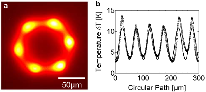
Figure 2: (color online) Demonstration experiment. (a) A circular thermal wave is created in water by a moving focus of an infrared laser. The temperature is inferred by stroboscopic imaging of a temperature-sensitive fluorescent dye. (b) Peak temperature along the circumference. A sinusoidal fit yields a temperature amplitude of $\delta T_{0}=3.8\pm 0.5\,\text{K}$.

The thermal wave is generated by a scanning laser spot. Six individual temperature peaks are created by a circular pattern of radius $R$= 50 µm with a base frequency of 30 kHz. The frequency is faster than the thermal relaxation time, which is dominated by the vertical heat currents and determined to 0.21 ms using a finite element calculation. As result, a steady thermal wave of six points is generated, measured in Fig. 2. The points are rotated using a slower shift frequency $f_{S}=0.2\ldots 2\,\text{kHz}$. The result is a circular thermal wave with velocity $u=f_{S}\times 2\pi R/6=10\ldots 100\,\text{mm/s}$.

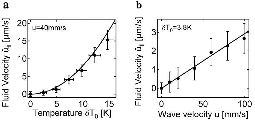
Figure 3: (color online) Experiment versus theory. (a) The fluid velocity scales quadratically with the amplitude of the thermal wave $\delta T_{0}$. (b) The speed increases linearly with the velocity $u$ of the thermal wave. Measurements are given as dots, the theory as solid lines with the geometrical prefactor determined in Ref. Kraus (2007). Error bars are standard errors.

Fluid velocities are measured by single particle tracking of 80 pM of 1 µm diameter silica beads (PSi-G1.0, Kisker). Particle velocities could be well discriminated from Brownian diffusion by tracking 5 independent particles over 10µm with a positional error of 1 µm. The peak velocity of the parabolic flow profile was measured by selecting the beads in the chamber center. The experimental values were multiplied by $2/3$ to compare with the chamber-averaged theoretical values. Optical trapping or thermophoresis would move the tracer particles with the thermal wave, opposite to the observed flow direction. Under the experimental conditions, both effects would yield similar attractive forces. However, control experiments in heavy water with its 100-fold decreased absorptive heating only revealed moderate attraction into the illuminated ring, but no pumping movement along it (<0.13 µm/s). This indicates that the particles are ideal tracers of the fluid motion at the used focus size Duhr et al. (2006).

With the above described temperature pattern and a thermal wave velocity of $u=100\,\text{mm/s}$ we measure a peak fluid flow of $v_{\text{fl}}^{\text{exp}}=2.7\pm 0.5$ µm/s. We expect from the wide wave solution, Eq. 9, a fluid velocity of $v_{\text{fl}}^{\text{theo}}=4.77$ µm/s. Applying the complete analytical solution Kraus (2007) or the Femlab result yields $v_{\text{fl}}^{\text{FEM}}=2.88$ µm/s which describes the experimental result quantitatively.

Two parameter variations further confirm the theoretical model (Fig. 3). The dependence on the temperature amplitude $\delta T_{0}$ exhibits a parabolic dependence (Fig. 3 a) as expected theoretically by Eq. (9). Furthermore, the fluid velocity scales linearly with the velocity $u$ (Fig. 3 b) of the thermal wave as predicted (solid lines). We therefore find experimentally that a circular thermal wave triggers a fluid flow according to the theoretical description.

To conclude, we showed that a thermal wave can move a fluid by the nonlinear combination of the temperature-dependent density and viscosity. While the obtainable fluid velocities are small at present, future improvements could allow microfluidic applications.